Information Theoretic Measures to Infer Feedback Dynamics in Coupled Logistic Networks

Abstract

A process network is a collection of interacting time series nodes, in which interactions can range from weak dependencies to complete synchronization. Between these extremes, nodes may respond to each other or external forcing at certain time scales and strengths. Identification of such dependencies from time series can reveal the complex behavior of the system as a whole. Since observed time series datasets are often limited in length, robust measures are needed to quantify strengths and time scales of interactions and their unique contributions to the whole system behavior. We generate coupled chaotic logistic networks with a range of connectivity structures, time scales, noise, and forcing mechanisms, and compute variance and lagged mutual information measures to evaluate how detected time dependencies reveal system behavior. When a target node is detected to receive information from multiple sources, we compute conditional mutual information and total shared information between each source node pair to identify unique or redundant sources. While variance measures capture synchronization trends, combinations of information measures provide further distinctions regarding drivers, redundancies, and time dependencies within the network. We find that imposed network connectivity often leads to induced feedback that is identified as redundant links, and cannot be distinguished from imposed causal linkages. We find that random or external driving nodes are more likely to provide unique information than mutually dependent nodes in a highly connected network. In process networks constructed from observed data, the methods presented can be used to infer connectivity, dominant interactions, and systemic behavioral shift.

1. Introduction

A process network is a collection of time series variables that interact at different time scales [1]. Each time series variable is a node in the network, and nodes are linked through time dependencies. Synapses in the human brain, industrial processes in a factory, or climate-vegetation-soil relationships can all be studied as process networks [2,3,4]. In each of these examples, a time dependent relationship between the history of a source node and current state of a target node defines a network link that has some strength, time scale, and directionality. A whole-network property such as average node degree, average link strength, or dominant time scale can define a “system state”. It is important to correctly detect and interpret these links to reveal aspects of a network such as forcing structure, feedback, and shifts or breakdowns of links over time. Breakdowns or shifts in links could indicate changes in network response due to perturbations or gradual changes in the environment. With this framework, questions relating to threshold responses and overall health of a system can be readily addressed, and the system as a whole can be better understood. Process network construction requires accurate detection of time dependent links and evaluation of their importance and strength in terms of network behavior.

Studies on networks composed of oscillators and coupled chaotic logistic equations have shown that interacting nodes exhibit a wide range of dynamics depending on node coupling strengths, imposed time dependencies, and forcing [5,6,7,8,9,10]. Time series nodes can range from being unconnected to exhibiting various types of synchronization such as complete, lagged, general, or phase synchronization. Complete and lagged synchronized nodes have coincident states either simultaneously or at a time delay, phase synchronized nodes are locked in phase but vary in amplitude, and generally synchronized nodes have some functional relationship [8]. In chaotic logistic networks, the potential for these dynamics depends on delay (τ) distribution, coupling strength (ϵ) and connectivity ($K_f$) [5,6,9]. For strongly connected networks, synchronization is largely independent of the connection topology (Δ). As a result, networks with different connection topologies, such as random, scale free, and small-world, all achieve complete synchronization at a threshold connectivity as measured by average node degree multiplied by node coupling strength ϵ [6]. When delays (τ) between nodes are uniform, the network synchronizes to a chaotic trajectory [6]. When delays are distributed over multiple τ values, the network synchronizes to a steady state, or fixed point value [6]. At lower connectivities, the network displays a range of dynamics. The complexity of network behavior increases with the incorporation of stochastic forcing or noise.

In observed or measured process networks, nodes are likely to exhibit a combination of deterministic behavior due to functional dependencies and stochastic behavior due to random influences. In this study, we aim to identify time dependencies within networks of various structures, in addition to classifying networks in terms of their forcing-feedback mechanisms. Shifts in time dependencies or driving nodes in process networks could identify behavioral shifts in response to perturbations. These shifts could indicate alterations in important structural or functional components of the system.

Identification of coupling in real networks relies on statistical measures designed to capture the diversity of time dependent interactions. Metrics used to detect synchronization and time dependencies between nodes include variance and correlation measures [5,6,9], information theory measures [2,3], convergent cross mapping [11], coupling spectrums [12], graphical models [13,14], and various others [4]. Variance (${\sigma }^2$) measures between nodes and over time estimate relative levels of synchronization between nodes and identify the existence of complete synchronization to a single trajectory or fixed point [5,6,9]. Information theory measures such as entropy $H\left(X\right)$, mutual information $I(X;Y)$, transfer entropy $TE(X\to Y)$ [15], and partial mutual information [16,17] quantify uncertainty of node states and reductions in uncertainty given other node states. Information theory measures have been applied in ecohydrology [1,2,18], neuroscience [19,20], and industrial engineering [3], among others, to identify transmitters and receivers of information in addition to feedback within a network. When contributions from multiple “source” nodes to a “target” node are considered, shared information can be decomposed into redundant, unique and synergistic components [21]. Redundant information is the information shared between every source node and the target node, and unique information is that which only a single source shares with the target. In some cases, the knowledge of two source nodes may provide information to a target node that is greater than the union of the information provided by both sources individually, thus providing synergistic information.

The objective of this article is to determine the additional knowledge that information theory measures can provide over variance measures concerning process network behavior, such as distinguishing between types of drivers, locating feedback, and identifying redundant versus unique sources of information. How well do information theory measures capture imposed network dynamics? When a time dependent link is identified, is it critical in terms of network function, or redundant with other interactions? Time dependencies identified in real process networks could be either important aspects of system health or functioning, or redundant due to induced feedback. Although the existence of feedback within process networks can obscure what is a “cause” versus an “effect” and prevent detection of causality, the estimation of redundancy can identify groups of redundant links [22] which can then be further evaluated in terms of their contributions to system behavior.

This study uses a method to compute information theory measures that does not assume time series variables to follow a Gaussian distribution, and performs well given limited datasets with as few as 200 data points. This minimization of the data requirement is valuable because data used to form real world process networks are often sparse, fragmented, or noisy [19]. There are several proposed methods to directly evaluate redundancy, synergy, and unique information [20,21,23,24] that each have advantages and disadvantages in their interpretation [24,25,26]. Here we instead use combinations of established information theory measures that reveal multiple aspects of information transfers.

We create chaotic-logistic networks with a range of τ-distributions, coupling strengths ϵ, topologies Δ, and levels of noise, and compare information theory and variance measures to the imposed network structures. We evaluate our methods in terms of correctly identified links, or statistically significant detections of information measures that correspond to imposed time dependencies. In a network of observed time series data, structural properties such as driving nodes, node degrees, and coupling strengths are generally unknown and may change over time. However, process network construction can reveal some of this structure, and temporal changes in detected links indicate shifts in properties. In addition, comparisons of process networks can detect differences between inputs and outputs of a model or between measured and simulated variables. Through this analysis of generated network dynamics, we improve our ability to identify and interpret real-world process networks that range from uncoupled to completely synchronized.

2. Methods: Definition of Metrics

We evaluate network behavior with several measures that capture variability and time-dependent interactions. The standard deviation between node values, ${\sigma }_{nodes}$, indicates synchronization between nodes [5]. In a network composed of $i=1\dots N$ nodes and $t=1\dots .n$ time steps per node,

$${\sigma }_{nodes}=\frac{1}{n}\sum _{t=1}^n\left[{\left(\frac{{\sum }_{i=1}^N{(x_i\left(t\right)-\overline{x}\left(t\right))}^2}{N-1}\right)}^{1/2}\right]$$

(1)

For complete synchronization, ${\sigma }_{nodes}=0$. The standard deviation between time steps averaged over the N nodes, ${\sigma }_{time}$, indicates the temporal variation of nodes [5].

$${\sigma }_{time}=\frac{1}{N}\sum _{i=1}^N\left[{\left(\frac{{\sum }_{t=1}^n{(x_i\left(t\right)-\widehat{x_i})}^2}{n-1}\right)}^{1/2}\right]$$

(2)

In these metrics, $\overline{x}\left(t\right)$ is the mean node value at time t, and $\widehat{x_i}$ is the mean temporal value of node i. If both ${\sigma }_{nodes}=0$ and ${\sigma }_{time}=0$, all the nodes in the network are at the same fixed point value for all time steps. If ${\sigma }_{nodes}>0$ and ${\sigma }_{time}=0$, nodes are at different fixed point values. Finally, if ${\sigma }_{nodes}=0$ and ${\sigma }_{time}>0$, nodes are completely synchronized to each other but vary with time [5]. These measures can also be applied to any pair of nodes or subsystems within a larger network, and are useful when comparing networks to a reference or baseline condition. Since ${\sigma }_{nodes}$ and ${\sigma }_{time}$ depend on the range of values ($x_i\left(t\right)$) taken by nodes in the network, the significance of any $\sigma >0$ is difficult to evaluate without further knowledge of the range of possible network behaviors.

Information theory measures involve comparing probability density functions (pdfs) of nodes rather than their magnitudes. Shannon entropy $H\left(X\right)$ quantifies the uncertainty or variability of a node. $H\left(X\right)$ can be computed and normalized to between 0 and 1 by dividing by the upper bound $log\left(\mathcal{N}\right)$, where $\mathcal{N}$ is the chosen number of bins into which the pdf $p\left(x\right)$ is discretized.

$$H\left(X\right)=\sum _{k=1}^{\mathcal{N}}p\left(x_k\right)log\left[\frac{1}{p\left(x_k\right)}\right]$$

(3)

Mutual information $I(X_a;X_b)$ is the reduction in uncertainty of node $X_a$ given knowledge of the state of another variable $X_b$, and is computed from the joint pdf.

$$I(X_a;X_b)=\sum p(x_a,x_b)log\left[\frac{p(x_a,x_b)}{p\left(x_a\right)p\left(x_b\right)}\right]=H\left(X_a\right)-H\left(X_a\right|X_b)$$

(4)

Lagged mutual information $I_{\tau }=I(X_a(t-{\tau }_a);X_{tar}\left(t\right))$ quantifies the information shared between a target node $X_{tar}$ and the ${\tau }_a$-lagged history of a source node $X_a$. Although I is a symmetric quantity, $I_{\tau }$ introduces a directionality if we assume that past node states inform future states, and not vice versa. In other words, we consider past node states to be “sources” and a future state to be a “target”. In a network of interacting nodes, multiple sources in the form of different nodes or a single node at different time scales can provide information to a single “target” node. The total lagged $I_{\tau }$ shared by two sources ($X_{s1}$ and $X_{s2}$) to a target ($X_{tar}$) is the mutual information between one source and the target added to the conditional mutual information as follows:

$$I(X_{tar};X_{s1},X_{s2})=I(X_{tar};X_{s2})+I(X_{tar};X_{s1}|X_{s2})$$

(5)

Using the partial information decomposition approach [21,27], we see that this shared information between two sources and the target can be partitioned into elements as follows:

$$I(X_{tar};X_{s1},X_{s2})=U_{s1}+U_{s2}+R_{s1,s2}+S_{s1,s2}$$

(6)

$$I(X_{tar}\left(t\right);X_{s1}(t-{\tau }_{s1}))=U_{s1}+R_{s1,s2}$$

(7)

$$I(X_{tar}\left(t\right);X_{s2}(t-{\tau }_{s2}))=U_{s2}+R_{s1,s2}.$$

(8)

In Equations (6)–(8), $U_{s1}$ and $U_{s2}$ represent the unique information that only $X_{s1}(t-{\tau }_{s1})$ and $X_{s2}(t-{\tau }_{s2})$, respectively, share with $X_{tar}\left(t\right)$, $S_{s1,s2}$ is the synergistic information that arises only from the knowledge of both $X_{s1}(t-{\tau }_{s1})$ and $X_{s2}(t-{\tau }_{s2})$ together, and $R_{s1,s2}$ is the redundant information that is provided by either source node separately.

We see from substituting Equations (8) and (6) into Equation (5) that the conditional information term $I(X_{tar};X_{s1}|X_{s2})$ is equivalent to $U_{s1}+S_{s1,s2}$, or the unique information component of one source node and the synergistic information due to the knowledge of both sources. The same result can be obtained by observing that conditional mutual information is equal to the interaction information or co-information [21,28,29] ($II=I(X_{tar}\left(t\right);X_{s1}(t-{\tau }_{s1});X_{s2}(t-{\tau }_{s2}))=S_{s1,s2}-R_{s1,s2}$) added to the mutual information ($U_{s1}+R_{s1,s2}$). A positive interaction information ($II>0$) indicates that synergy dominates over redundancy in the partitioning of shared information [21]. An $II<0$ indicates dominant redundancy, or that the knowledge of any one variable “explains” correlation between the other two [29]. Conditional $I_{\tau }$ (i.e., $I(X_{tar};X_{s1}|X_{s2})$) is also referred to as partial information, since it represents the part of the total mutual information that is not contained in the second source node ($X_{s2}$) [17]. The conditional $I_{\tau }$ is computed between two sources and a target node as follows:

$$I(X_{tar};X_{s1}|X_{s2})=\sum _{\begin{array}{c}{x}_{tar}\left(t\right),\\ x_{s1}(t-{\tau }_{s1}),\\ x_{s2}(t-{\tau }_{s2})\end{array}}p(x_{tar}\left(t\right),x_{s1}(t-{\tau }_{s1}),x_{s2}(t-{\tau }_{s2}))log\left[\frac{p(x_{tar}\left(t\right),x_{x2}(t-{\tau }_{s2}),x_{s1}(t-{\tau }_{s1}))}{p(x_{tar}\left(t\right),x_{s2}(t-{\tau }_{s2})}\right]$$

(9)

In Equations (5) and (9), if we consider the special case where one of the source nodes $X_{s2}$ is the lagged history of the target node $X_{tar}$ itself (i.e., $X_{s2}(t-{\tau }_{s2})=X_{tar}(t-{\tau }_{tar})$), the conditional mutual information term is equivalent to the transfer entropy $TE(X_{s1}(t-{\tau }_{s1})\to X_{tar})$. Transfer entropy [15] is the reduction in uncertainty of a node $X_{tar}$ due to the knowledge of the $(t-{\tau }_{s1})$ history of another node $X_{s1}$ that is not already accounted for in the $(t-{\tau }_{tar})$ history of $X_{tar}$ [2,18]. $TE$ is often interpreted as the amount of predictive information transferred between two processes [30]. Some formulations of $TE$ involve consideration of block lengths l and k of the histories of the transmitting node $X_{s1}$ and receiving node $X_{tar}$, respectively. However, the values of l and k are generally set equal to 1 so as to not impose additional data requirements for the computation of a higher dimensional pdf [7,15,31]. In this study, we relax the usual assumption in transfer entropy computations that predictive information from a source node is only conditioned on the target node’s history. $T\equiv I(X_{tar};X_{s1}|X_{s2})$ provides a generalization of $TE$ that conditions the predictive information of the time dependency of any source, including the history of the target node itself.

In this paper, we establish network links by computing lagged mutual information $I_{\tau }$ using Equation (4) between each potential source and target node for a range of time delays. To test for statistical significance of the detected value, we randomly shuffle the target node $X_{tar}$ to destroy time correlations while retaining other properties of the time series data [2,32,33]. We compute 100 values of $I_{\tau \mathit{shuffled}}$, and perform a hypothesis test at a 99% confidence level. If the detected value is less than $I_{\tau \mathit{shuffled},\mathit{mean}}+3*{\sigma }_{\mathit{shuffled}}$, we dismiss the detected link as not significant.

After establishing time dependent links in the network, we compute the total and conditional $I_{\tau }$ provided by each pair of sources to every target node using Equations (9) and (5). We define $T/I$ as an index to measure the non-redundant component of each link as a function of conditional and total shared information as follows:

$$\frac{T}{I}(X_{s1}\to X_{tar})=\underset{X_{s2}}{min}\left[\frac{I(X_{tar};X_{s1}|X_{s2})}{I(X_{tar};X_{s1},X_{s2})}\right]$$

(10)

where

$$\frac{I(X_{tar};X_{s1}|X_{s2})}{I(X_{tar};X_{s1},X_{s2})}=\frac{U_{s1}+S_{s1,s2}}{U_{s1}+U_{s2}+S_{s1,s2}+R_{s1,s2}}$$

(11)

Computation of $T/I$ requires a pairwise evaluation of sources for each detected target node in the network. For a link between $X_{tar}$ and a source $X_{s1}$, minimization across each each alternate source $X_{s2}$ provides a conservative measure of the unique and synergistic components of the link. In the absence of synergistic relationships, if a source $X_{s1}$ is completely redundant due to another source (i.e., $U_{s1}=0$ and $S_{s1,s2}=0$), then $T/I=0$. If $X_{s1}$ is the only source or is much stronger than all other sources (i.e., $U_{s1}\gg U_{s2}$), then $T/I$ approaches 1. Therefore, $T/I$ characterizes the relative amount of unique or synergistic information provided by a link as originally determined based on statistically significant $I(X_{tar};X_{s1})$. While $I(X_{tar};X_{s1})$ detects a single time dependent link, conditioning on other dependencies allows for detection of unique and redundant linkages [16,34]. High $T/I$ values can also result from synergistic relationships, where much more information is shared by two sources together than either shares separately. Other methods of detecting or eliminating redundant sources include direct transfer entropy [3] or causation entropy [35], which involve 4D pdf estimation to condition on multiple source nodes.

We use the Kernel Density Estimation (KDE) [19,22,36] method to estimate the 3D pdf ($p(x_{tar}\left(t\right),x_{s1}(t-{\tau }_{s1}),x_{s2}(t-{\tau }_{s2})$) required to compute conditional $I_{\tau }$ and the 2D and 1d pdfs needed for $I_{\tau }$ and H after testing several techniques [2,7,12,19] on two-node networks of $50\le n\le 2000$ data points and varying noise levels. The kernel estimator at a grid point or location y given $Y_{i=1\dots .n}$ observations is defined as [36]:

$$\widehat{p}\left(y\right)=\frac{1}{n{h}^d}\sum _{i=1}^n\kappa \left[\frac{1}{h}(y-Y_i)\right]$$

(12)

The multivariate Epanechnikov kernel $\kappa ={\kappa }_e$ [36] is as follows:

$${\kappa }_e\left(x\right)=\left\{\begin{array}{cc}\hfill \frac{1}{2}{c}_d^{-1}(d+2)(1-y^{T}y)& \mathrm{if} y^{T}y<1\hfill \\ \hfill 0& \mathrm{otherwise}\hfill \end{array}\right.$$

(13)

in which d is the dimension of the $pdf$, $c_d$ is the volume of a d-dimensional unit sphere, and n is the number of observations. The optimal window width h for the kernel is chosen to vary with n and d based on [36] as follows:

$$h_{opt}=\left\{\begin{array}{cc}\hfill 1.06\sigma n^{-1/5}& \mathrm{if}d=1\hfill \\ \hfill 1.77\sigma n^{-1/6}& \mathrm{if}d=2\hfill \\ \hfill 2.78\sigma n^{-1/7}& \mathrm{if}d=3\hfill \end{array}\right.$$

(14)

in which σ is the standard deviation of the data. We evaluate the kernel at $\mathcal{N}=35$ evenly spaced grid points (y) in each dimension. The KDE method performed similarly to fixed-binning [2,19] and partitioning methods [19] for large data sets, but the smoothing of the pdf due to the kernel improved performance for small data sets with $n<200$.

3. Results: 2-Node Networks

To assess whether our estimates of $I_{\tau }$ and $T/I$ accurately identify time dependencies and distinguish between types of forcing, we first consider three bivariate cases. In each case, node $X_1$ forces another node $X_2$ at a time lag of ${\tau }_{1,2}=3$ via a chaotic logistic equation. However, the driving node $X_1$ is established in different ways.

3.1. Logistic Forcing

For a chaotic logistic forcing case, $X_1$ is an independent chaotic logistic equation, and node $X_2$ is a chaotic logistic function dependent on the ${\tau }_{1,2}=3$ lagged history of $X_1$ (illustration in Figure 1a, left), that is:

$$\begin{array}{c}\hfill X_1\left(t\right)=f\left(X_1(t-1)\right)\\ \hfill X_2\left(t\right)=f\left(X_1(t-3)\right)\end{array}$$

(15)

where $f\left(X\right)=aX(1-X)$ with $a=4$. This configuration results in statistically significant detected $I_{\tau }$ between all node pairs (Figure 1a). Since $X_1$ is self-driven at a lag of ${\tau }_{1,1}=1$, and forces $X_2$ at a lag of ${\tau }_{1,2}=3$, we detect the dominant dependency from $X_1$ to $X_2$ at a lag of ${\tau }_{1,2}-{\tau }_{1,1}=2$ instead of the imposed ${\tau }_{1,2}=3$. The self-feedback of $X_1$ is reflected in $X_2$, and we see from the time series (Figure 1a Left) that the nodes are shifted copies of each other. The proportion $T/I$ is rather low between all pairs (Figure 1a), indicating no single source to a target is extremely strong compared to others, thus sources are likely to contain redundancies ($R_{s1,s2}>0$). In fact, we know from the time series that any information shared between $X_1$ and $X_2$ is completely redundant given their own histories. In other words, there is no S or U component since the history of each node contains complete predictive information. This should result in $T/I=0$, since $U_s=0$ and $S=0$. However, we see from Figure 1a that $T/I>0$. This results from the necessarily empirical estimation of the pdf.

Figure 1. two-node networks with different forcings imposed on node $X_1$ ($n=2000$ and $n=50$). Node $X_2$ is always a function of the ${\tau }_{1,2}$ lagged history of $X_1$. Left: red arrows indicate forcing, and blue dotted arrows indicate induced feedback that was also detected using information measures. An example time series is shown below illustrations. Middle, Right: Information measures $I_{\tau }$ and $T/I$ for each source indicate strength and uniqueness of detected dependencies (yellow indicates high $T/I$) for $n=2000$ data points (middle) and $n=50$ (right). (a) Logistic equation forcing case: dominant transfer detected from $X_1$ to $X_2$ at a lag equal to ${\tau }_{1,2}-{\tau }_{1,1}$, and self-feedback on $X_2$ reflects that of $X_1$; (b) Feedback forcing case: I and $T/I$ detect imposed links, and self-feedback at lag of ${\tau }_{2,1}+{\tau }_{1,2}$; $T/I<0.5$ for all links, indicating high level of redundancy (c) Random forcing case: imposed link from $X_1$ to $X_2$ detected. $T/I=1$ indicates that this link constitutes unique shared information.

Figure 1. two-node networks with different forcings imposed on node $X_1$ ($n=2000$ and $n=50$). Node $X_2$ is always a function of the ${\tau }_{1,2}$ lagged history of $X_1$. Left: red arrows indicate forcing, and blue dotted arrows indicate induced feedback that was also detected using information measures. An example time series is shown below illustrations. Middle, Right: Information measures $I_{\tau }$ and $T/I$ for each source indicate strength and uniqueness of detected dependencies (yellow indicates high $T/I$) for $n=2000$ data points (middle) and $n=50$ (right). (a) Logistic equation forcing case: dominant transfer detected from $X_1$ to $X_2$ at a lag equal to ${\tau }_{1,2}-{\tau }_{1,1}$, and self-feedback on $X_2$ reflects that of $X_1$; (b) Feedback forcing case: I and $T/I$ detect imposed links, and self-feedback at lag of ${\tau }_{2,1}+{\tau }_{1,2}$; $T/I<0.5$ for all links, indicating high level of redundancy (c) Random forcing case: imposed link from $X_1$ to $X_2$ detected. $T/I=1$ indicates that this link constitutes unique shared information.

Figure 2a shows the data attractor (points $[x_2\left(t\right),x_1(t-2),x_1(t-3)]$) and estimated pdfs used to compute $I_{\tau }$ and $T/I$ at the delay ${\tau }_{1,2}=3$. From the 3D pdf (Figure 2a Middle), we see that there is a linear relationship (1:1 line) between $X_1(t-2)$ and $X_2\left(t\right)$ indicating that the nodes have coincident states at a time lag of 2, thus a dominant $I_{\tau }$ link at that lag. There is a parabolic relationship between $X_1(t-3)$ and $X_2\left(t\right)$. Due to this structure of the 3D pdf where $X_1(t-2)$ predicts $X_2\left(t\right)$ more directly than the imposed link $X_1(t-3)$, we detect non-zero $T/I$. In other words, a unique component of information is detected between $x_1(t-2)$ and $x_2\left(t\right)$. However, the low $T/I$ for all links indicates that each target node receives information from multiple sources, or a single source at multiple time lags. If we assume that sources do not provide synergistic information, $T/I<0.5$ for all dependencies indicates that the stronger sources contain significant redundancies with weaker sources. This assumption is valid for our generated networks, since multiple source node histories do not inform the target beyond the union of their individual contributions.

Figure 2. Empirical pdfs for each of the two-node network cases for $n=2000$ data points (left, middle) and $n=50$ (right). Red stars indicate data points, blue circles are grid points $(i,j,k)$ for which $pdf(i,j,k)>0.0001$. Left: 2-dimensional pdfs used to compute $I_{\tau }$ between $X_1(t-3)$ and $X_2\left(t\right)$. Middle, Right: 3-dimensional pdf used to compute corresponding $T/I$ of link. (a) Logistic forcing: $X_1(t-2)$ and $X_2\left(t\right)$ are completely synchronized (1:1 line), so there is redundancy in the transfer from $X_1(t-3)$ to $X_2\left(t\right)$; (b) Feedback forcing: both the histories of $X_1$ and $X_2$ inform $X_2\left(t\right)$ due to feedback. In (a) and (b), significant $T/I$ is still detected due to empirical estimation of the 3D pdfs; (c) Random forcing: knowledge of $X_2(t-1)$ (or any other lagged node history) conveys no information concerning $X_2\left(t\right)$, thus there are no other significant links and $T/I=1$.

Figure 2. Empirical pdfs for each of the two-node network cases for $n=2000$ data points (left, middle) and $n=50$ (right). Red stars indicate data points, blue circles are grid points $(i,j,k)$ for which $pdf(i,j,k)>0.0001$. Left: 2-dimensional pdfs used to compute $I_{\tau }$ between $X_1(t-3)$ and $X_2\left(t\right)$. Middle, Right: 3-dimensional pdf used to compute corresponding $T/I$ of link. (a) Logistic forcing: $X_1(t-2)$ and $X_2\left(t\right)$ are completely synchronized (1:1 line), so there is redundancy in the transfer from $X_1(t-3)$ to $X_2\left(t\right)$; (b) Feedback forcing: both the histories of $X_1$ and $X_2$ inform $X_2\left(t\right)$ due to feedback. In (a) and (b), significant $T/I$ is still detected due to empirical estimation of the 3D pdfs; (c) Random forcing: knowledge of $X_2(t-1)$ (or any other lagged node history) conveys no information concerning $X_2\left(t\right)$, thus there are no other significant links and $T/I=1$.

When the pdf is estimated based on 50 data points instead of 2000 (Figure 1a Right), we detect statistically significant but lower $I_{\tau }$ compared to the $n=2000$ point case, and similar values of $T/I$. Comparison of the 3D pdfs in Figure 2a shows that fewer data points results in more spread of the empirical pdf due to the kernel estimator, and weaker detection of information measures (Figure 1 Right).

3.2. Feedback Forcing

For a feedback forcing case, each node is a function of the history of the other node at lags ${\tau }_{2,1}=4$ and ${\tau }_{1,2}=3$ (illustration in Figure 1b), that is:

$$\begin{array}{c}\hfill X_1\left(t\right)=f\left(X_2(t-4)\right)\\ \hfill X_2\left(t\right)=f\left(X_1(t-3)\right)\end{array}$$

(16)

Similar to the logistic forcing case, this case results in high detected $I_{\tau }$ and relatively low $T/I$ between all the node pairs (Figure 1b). This indicates that the nodes are highly coupled, and are predictable given knowledge of either node at one of several time lags. This is also apparent given the high “self” $I_{\tau }$ for each node. We note that by substitution in Equation (16), each node can be written as a function of its own history, indicating complete source redundancy and $T/I=0$. However, we detect $T/I>0$ for the same reason as the previously discussed logistic forcing example. The strongest detected source to target links, in this case the second order polynomial relation between $X_1(t-3)$ and $X_2\left(t\right)$ (Figure 2b Left), is detected to have a unique component when compared to the weaker link (fourth order polynomial) between $X_2(t-7)$ and $X_2\left(t\right)$ (Figure 2b Middle). In other words, although $X_2(t-7)$ provides all predictive information regarding $X_2\left(t\right)$, $X_2\left(t\right)$ is a more simple function of $X_1(t-3)$, so we still detect statistically significant $T/I$ from source $X_1$ to target $X_2$ (Figure 1b Middle). When feedback is involved, it is not possible to distinguish between “drivers” and “receivers” within the network, but we can identify the existence of this feedback and its strengths and time scales. Similar to the logistic forcing case, reducing the number of data points to $n=50$ results in more spread of the $pdfs$ and weaker detection of $I_{\tau }$ (Figure 1b Right).

3.3. Random Noise Forcing

In the last two-node network example, $X_1$ is a time series of randomly generated uniform noise (illustration in Figure 1c Left), that is:

$$\begin{array}{c}{X}_1\left(t\right)=z\sim U(0,1)\hfill \\ X_2\left(t\right)=f\left(X_1(t-3)\right)\hfill \end{array}$$

(17)

This case results in statistically significant $I_{\tau }$ and $T/I=1$ from $X_1$ to $X_2$ at the imposed delay (Figure 1c Middle). The high $T/I$ indicates that the link is a dominant and unique source of information to the target $X_2$. Furthermore, since there are no other links detected with $I_{\tau }$, we can conclude that neither synergy nor redundancy exists because all shared information is unique to the sole source $X_1$. In other words, because $X_1$ forces $X_2$, and $X_1$ is randomly generated, no information about $X_2$ is encoded in any other source. The pdfs estimated to detect $I_{\tau }$ and $T/I$ in this case are shown in Figure 2c for the $n=2000$ and $n=50$ cases. From the pdfs, we observe that $X_2(t-1)$ and $X_2\left(t\right)$ are uncorrelated.

With these example cases, we show that information measures $T/I$ and $I_{\tau }$ capture imposed time dependencies and feedback, and can determine the partitioning of shared information between different source histories. When a randomly generated node drives another node, we detect high $T/I$ since there is no information provided by other sources, and all shared information between the source (random driver) and target (receiving) node is unique. When there is feedback involved, such as in the logistic and feedback forcing cases, high $I_{\tau }$ is detected between all node pairs, but $T/I$ is low due to increased redundancies. Although $T/I$ is often detected as significant due to pdfstructure and its estimation, it still provides an estimate of the dominance of redundancy versus unique information, particularly in the absence of synergy. Detection of high $T/I(X_{s1}\to X_{tar})$ in the case of multiple sources indicates that the source $X_{s1}$ is either unique or is highly synergistic with another source.

The two-node cases with chaotic logistic driving nodes and feedback illustrate the detection of multiple links between nodes that were not directly imposed. However, these links are due to the imposed time dependencies and can be considered to be induced feedback. In the chaotic logistic driving case, a time-dependent source node forces a target node, causing the target node to acquire the same time dependency given its own history. In the feedback example, the imposed bi-directional feedback causes each node to have a time dependency given its own history. This induced feedback occurs in highly connected networks and can propagate due to a single imposed bi-directional feedback or time dependency. Detected time dependencies that were not imposed could be characterized as “false positives” in link detection [37], but we note that these detections are expected due to the forcing-feedback structure.

In this section, each node was forced by either a chaotic logistic equation or uniform random noise. In networks of multiple interacting processes, a single node may respond to many variables. In the next section, we generate 10-node networks with $n=200$ time series points, in which nodes may be forced by various combinations of neighbors in addition to uniform random noise. We compute information and variance measures, and analyze synchronization and time dependencies as connectivity varies. As in the two-node cases, $I_{\tau }$ and $T/I$ measures detect dependencies between node pairs, but are also used to identify the larger connectivity structure of the network. When multiple source nodes and random noise influence a single target node, information measures between node pairs are more weakly detected. However, we show that these measures can correctly identify even weak interactions and reveal the forcing-feedback structure of a network.

4. Results: Coupled Chaotic Logistic Networks

Previous studies have determined that chaotic logistic network synchronization capacity in terms of σ measures (${\sigma }_{nodes}$ and ${\sigma }_{time}$) depends more on the delay (τ) distribution than network topology Δ [5,6,9]. For a range of Δ including small-world, scale-free, and random networks, increasing connectivity (increasing coupling strength or number of links) leads to synchronization of all connected nodes. The dynamics of the resulting synchronized trajectory depend on the τ-distribution [6]. Networks with uniform delays (e.g., $\tau =1$ for all linked nodes) synchronize to a single chaotic logistic trajectory. In contrast, networks with heterogenous delays (e.g., random $\tau \in \{1,10\}$ for linked nodes) synchronize to the fixed point ($x^{*}=1-1/a$) of the logistic equation. This type of synchronization occurs when nodes that receive from enough neighbors at different lags converge toward the fixed point $x^{*}$ and all nodes approach zero amplitude [38]. In terms of information theory measures, it has been found that information transfer can be used to predict synchronization and distinguish between origins of interaction fields, or types of forcing, in different types of generated networks [7].

In this section, we extend the forcing mechanisms introduced in the two-node examples to larger 10-node networks. A 10 node network is small enough for computation efficiency and to represent many systems of interest, and large enough to capture the complexity and synchronization that larger networks exhibit. We generated networks of between 5 and 50 nodes and observed that larger networks synchronize at lower connectivities, but display otherwise similar behavior. The networks are generated over a range of connectivities, with different proportions of chaotic logistic and uniform random noise forcing. We introduce randomness into the network through randomly generated “driving nodes” that act as controls, or through the addition of uniform random noise to each node in equal proportion. We compute information and variance measures for the generated networks, and use whole-network measures to summarize each individual case. In chaotic logistic networks with no random component, we observe the expected delay-dependent synchronization.

4.1. Network Formation

We generate networks using Equation (18), each with $N=10$ nodes of $n=200$ time series points per node, using the framework given as:

$$X_i\left(t\right)=(1-ϵ)f\left(X_i(t-1)\right)+\frac{(1-{ϵ}_z)ϵ}{k_i}\sum _{j=1}^N{w}_{j,i}\left[f\left(X_j(t-{\tau }_{j,i})\right)\right]+{ϵ}_zϵz.$$

(18)

In Equation (18), i and j are node indices, $f\left(X\right)\equiv aX(1-X)$, t is time step, $k_i$ is the in-degree of node i, w is the adjacency matrix ($w_{j,i}=1$ if $X_i$ is a function of $X_j$, $w_{j,i}=0$ otherwise), τ is the delay matrix associated with w, and z is a uniform random noise between 0 and 1. As in the two-node example, we set $a=4$ so that each individual $f\left(X_i\right)$ is in the chaotic regime.

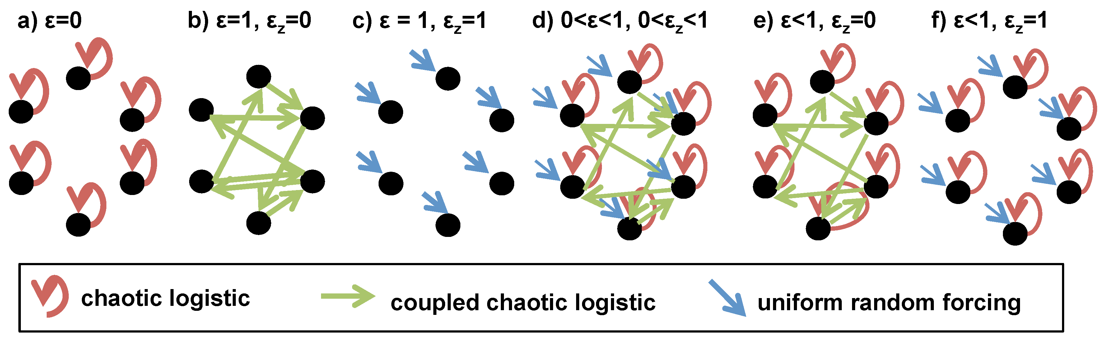
4.1.1. Network Forcing

The formulation of Equation (18) defines a node $X_i$ to be forced by (1) its own lagged history; (2) the lagged histories of connected nodes; and (3) random noise. The extents to which these components influence $X_i$ are defined by the coupling strengths ϵ and ${ϵ}_z$. For example, for $ϵ=1$ and ${ϵ}_z=0$, $X_i$ is solely a function of the histories of all $X_j$ for which $w_{j,i}=1$ (Figure 3b). If $ϵ=0$, each node is an independent chaotic logistic time series, since $X_i$ is only dependent on its own history (Figure 3a). If $ϵ=1$ and ${ϵ}_z=1$, the network is entirely composed of uniform random noise (Figure 3c). For values of $0<ϵ<1$ and $0<{ϵ}_z<1$, the network responds to all three types of forcing (Figure 3d).

In Equation (18), the imposed adjacency matrix w determines the interaction “field”, or set of nodes to which each node responds. The field is homogenous over time, but is different for each node. To explore the effect of external forcing, we introduce cases in which some of the 10 nodes are randomly generated time series ($n_{drivers}>0$). The remaining nodes are generated from Equation (18), and can be functions of both chaotic logistic and randomly generated nodes, depending on the adjacency matrix w. The noise component ${ϵ}_zϵz$ represents a different type of random forcing in that it affects each node in the network in equal proportion.

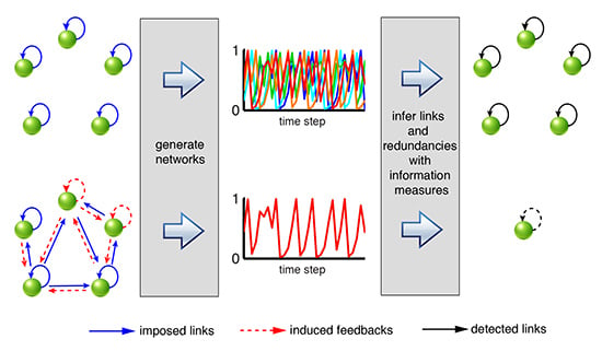
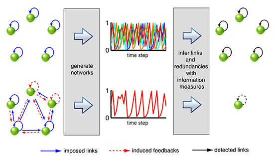
Figure 3. Illustration of network cases based on variations of Equation (18). (a) unconnected network driven by individual chaotic logistic equations; (b) network driven by chaotic logistic couplings; (c) unconnected network driven by random forcing; (d) network driven by combination of forcings according to $ϵ>0$ and ${ϵ}_z>0$; (e) network driven by combination of individual and coupled chaotic logistic equations; (f) unconnected network driven by random forcing and chaotic logistic equation.

Figure 3. Illustration of network cases based on variations of Equation (18). (a) unconnected network driven by individual chaotic logistic equations; (b) network driven by chaotic logistic couplings; (c) unconnected network driven by random forcing; (d) network driven by combination of forcings according to $ϵ>0$ and ${ϵ}_z>0$; (e) network driven by combination of individual and coupled chaotic logistic equations; (f) unconnected network driven by random forcing and chaotic logistic equation.

4.1.2. Network Topologies and Delays

Network topologies used to generate the adjacency matrix w include random and small world. Random networks are generated based only on a link probability p, while small world topologies [39] are bi-directional cyclic networks of degree 2 (each node transmits to and receives from $k=1$ neighbor on each side), and links are added randomly with probability p. A “theoretical weighted degree” K for each network type is the average number of incoming links per node multiplied by the coupling strength term $ϵ(1-{ϵ}_z)$. A fractional weighted degree $K_f=\frac{K}{N-1}$ is a measure of connectivity that ranges between 0 (unconnected nodes) and 1. At $K_f=1$, nodes are completely connected at maximum coupling strength, i.e., $ϵ(1-{ϵ}_z)=1$ and $p=1$.

Four specific classes of networks were tested, combining network topologies and delay distributions (Table 1). Cases 1 and 2 are random networks, while Cases 3 and 4 have small world topologies. Cases 1 and 3 have uniform delay distributions (${\tau }_{j,i}=1$ for $w_{j,i}=1$), and Cases 2 and 4 have random delay distributions (${\tau }_{j,i}\in \{1,10\}$ for $w_{j,i}=1$). As expected, we find that both topologies Δ behave similarly as network connectivity $K_f$ increases in terms of both standard deviation and information measures. As found in previous studies, we see that network behavior is most dependent on the τ-distribution and the connectivity $K_f$ rather than Δ. Cases 1 and 3 synchronize to a single chaotic logistic trajectory as $K_f$ is increased (Case 1 shown in Figure 4a), while Cases 2 and 4 synchronize to a fixed-point value as $K_f$ is increased (Case 2 shown in Figure 4b). Other network configurations tested include scale-free networks and higher degree ($k>1$) small world networks, all of which synchronized similarly according to their τ-distribution. Due to the similarities between network topologies, we show results for only Cases 1 and 2, the random network cases. Networks of various sizes from 5 to 50 nodes and observed similar results in terms of synchronization and detected information measures.

We canvas a range of parameters to form the adjacency matrices w and forcing structures and generate the subsequent process networks (Table 2). For each network, ϵ and ${ϵ}_z$ are constants (i.e., all nodes transmit and receive with equal coupling strengths), except for cases where $n_{drivers}>0$. In these cases, $n_{drivers}$ of the N total nodes are randomly generated nodes that only transmit information according to $w_{j,i}$. Over 40,000 distinct networks are generated (Table 2), and we compare several categories.

Table 1. Synchronization characteristics of four network cases composed of different topologies and delay (τ) distributions.

Case	Structure	τ-Distribution	$K_f$	Synchronization Type
1	random	uniform, $\tau =1$	$ϵ(1-{ϵ}_z)p$	chaotic trajectory
2	random	random, $\tau \in \{1,10\}$	$ϵ(1-{ϵ}_z)p$	fixed point
3	small world	uniform, $\tau =1$	$ϵ(1-{ϵ}_z)p+(1-p)\frac{2kϵ(1-{ϵ}_z)}{N-1}$	chaotic trajectory
4	small world	random, $\tau \in \{1,10\}$	$ϵ(1-{ϵ}_z)p+(1-p)\frac{2kϵ(1-{ϵ}_z)}{N-1}$	fixed point

Table 1. Synchronization characteristics of four network cases composed of different topologies and delay (τ) distributions.

Case	Structure	τ-Distribution	$K_f$	Synchronization Type
1	random	uniform, $\tau =1$	$ϵ(1-{ϵ}_z)p$	chaotic trajectory
2	random	random, $\tau \in \{1,10\}$	$ϵ(1-{ϵ}_z)p$	fixed point
3	small world	uniform, $\tau =1$	$ϵ(1-{ϵ}_z)p+(1-p)\frac{2kϵ(1-{ϵ}_z)}{N-1}$	chaotic trajectory
4	small world	random, $\tau \in \{1,10\}$	$ϵ(1-{ϵ}_z)p+(1-p)\frac{2kϵ(1-{ϵ}_z)}{N-1}$	fixed point

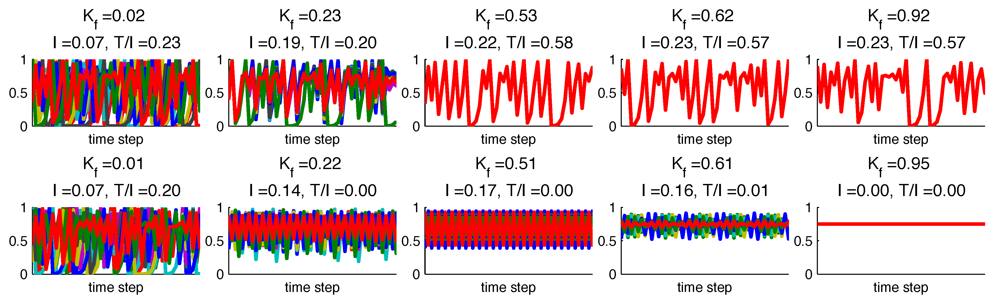
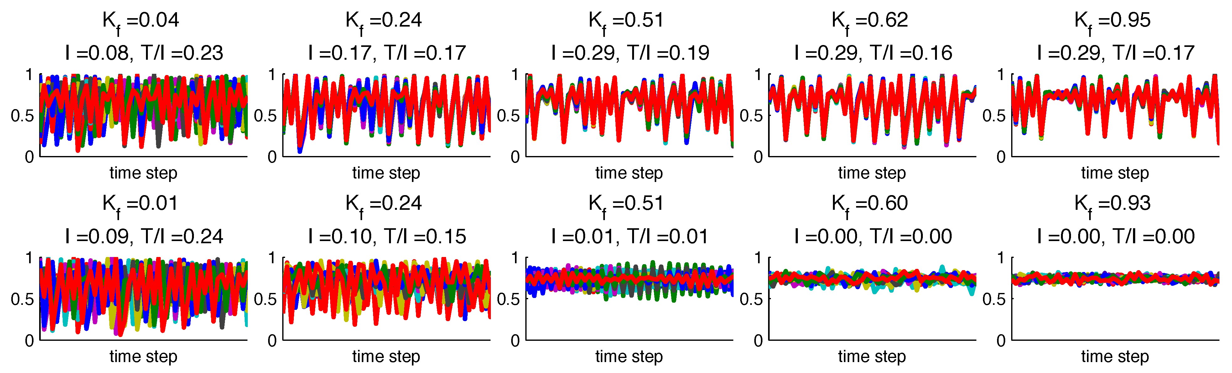
Figure 4. Time series (50 time steps shown) for several generated networks for (a) Case 1 with uniform ($\tau =1$) delay distribution and (b) Case 2 with random delay distribution. Both cases approach synchronization as $K_f$ increases.

Figure 4. Time series (50 time steps shown) for several generated networks for (a) Case 1 with uniform ($\tau =1$) delay distribution and (b) Case 2 with random delay distribution. Both cases approach synchronization as $K_f$ increases.

Table 2. 10 node network parameter range (42,336 total networks generated).

Parameter	Range of Values	Number of Cases
p	[0,0.05 $\dots$ 1]	21
ϵ	[0,0.05 $\dots$ 1]	21
${ϵ}_z$	[0, 0.01, 0.1, 0.5]	4
$n_{drivers}$	[0, 1 $\dots$ 5]	6
topology Δ	[random, small world $k=1$]	2
τ-distributions	[random, uniform]	2
total number of networks		42,336
cases with random Δ, $n_{drivers}=0$, ${ϵ}_z=0$		882

Table 2. 10 node network parameter range (42,336 total networks generated).

Parameter	Range of Values	Number of Cases
p	[0,0.05 $\dots$ 1]	21
ϵ	[0,0.05 $\dots$ 1]	21
${ϵ}_z$	[0, 0.01, 0.1, 0.5]	4
$n_{drivers}$	[0, 1 $\dots$ 5]	6
topology Δ	[random, small world $k=1$]	2
τ-distributions	[random, uniform]	2
total number of networks		42,336
cases with random Δ, $n_{drivers}=0$, ${ϵ}_z=0$		882

4.2. Synchronization and Information in Noise Free Networks

We first set ${ϵ}_z=0$ in Equation (18) to obtain a noise free network, and consider the range of coupling strengths $0<ϵ<1$ and link probability values $0<p<1$ (illustrations in Figure 3a,b,e). We see from the generated time-series data that nodes completely synchronize for high values of $K_f$ according to their τ-distributions (Figure 4). Observation of ${\sigma }_{nodes}$ (Figure 5a) leads to the same conclusion that both network cases synchronize to a single trajectory as $K_f$ increases, but at different rates. For Case 1 (uniform τ), complete synchronization to a time-varying trajectory is reached at $K_f=0.4$ (Figure 5a,d). Case 2 (random τ-distribution) synchronizes more gradually as $K_f$ increases, and is completely synchronized to a fixed-point trajectory for $K_f>0.7$ (Figure 5a,d).

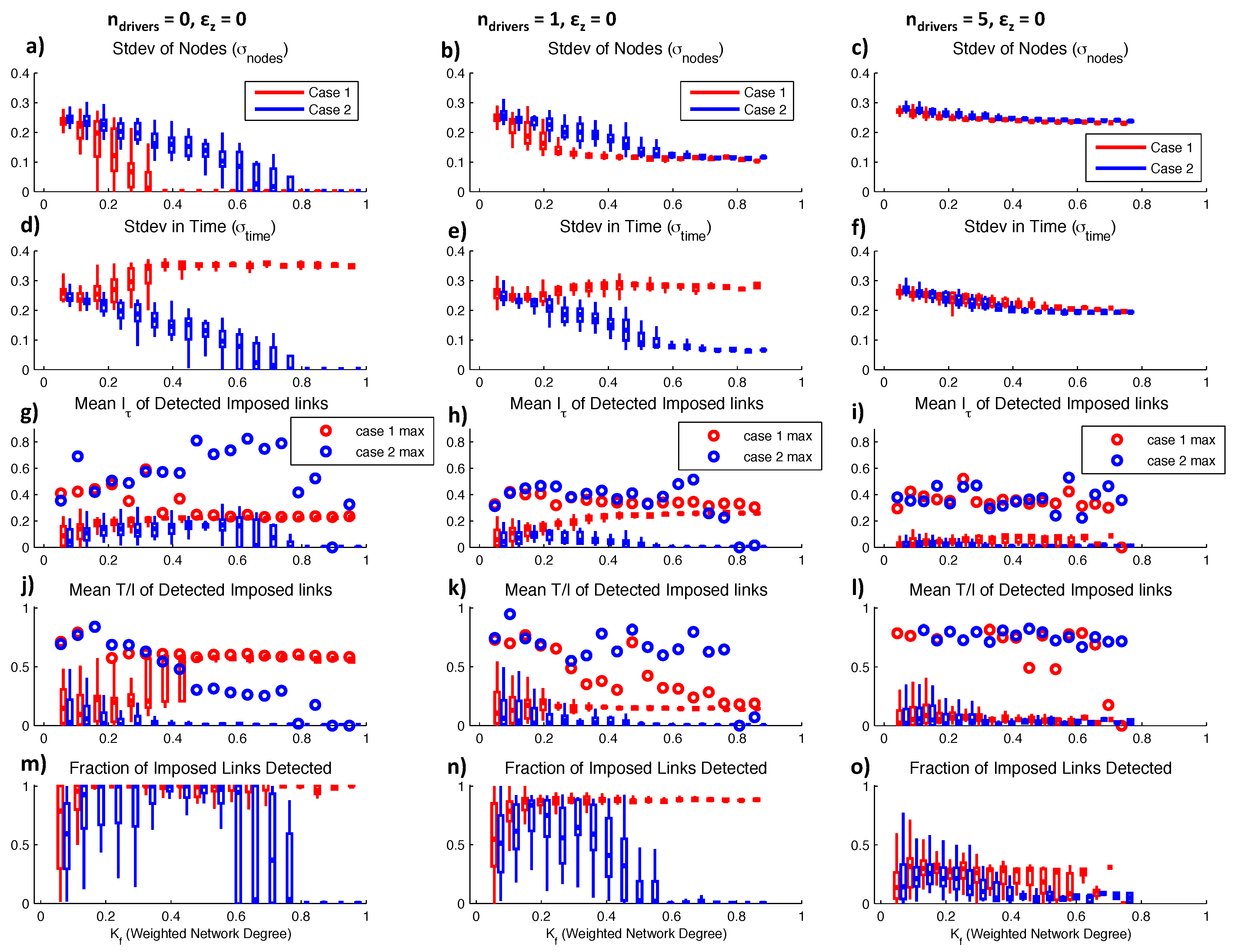
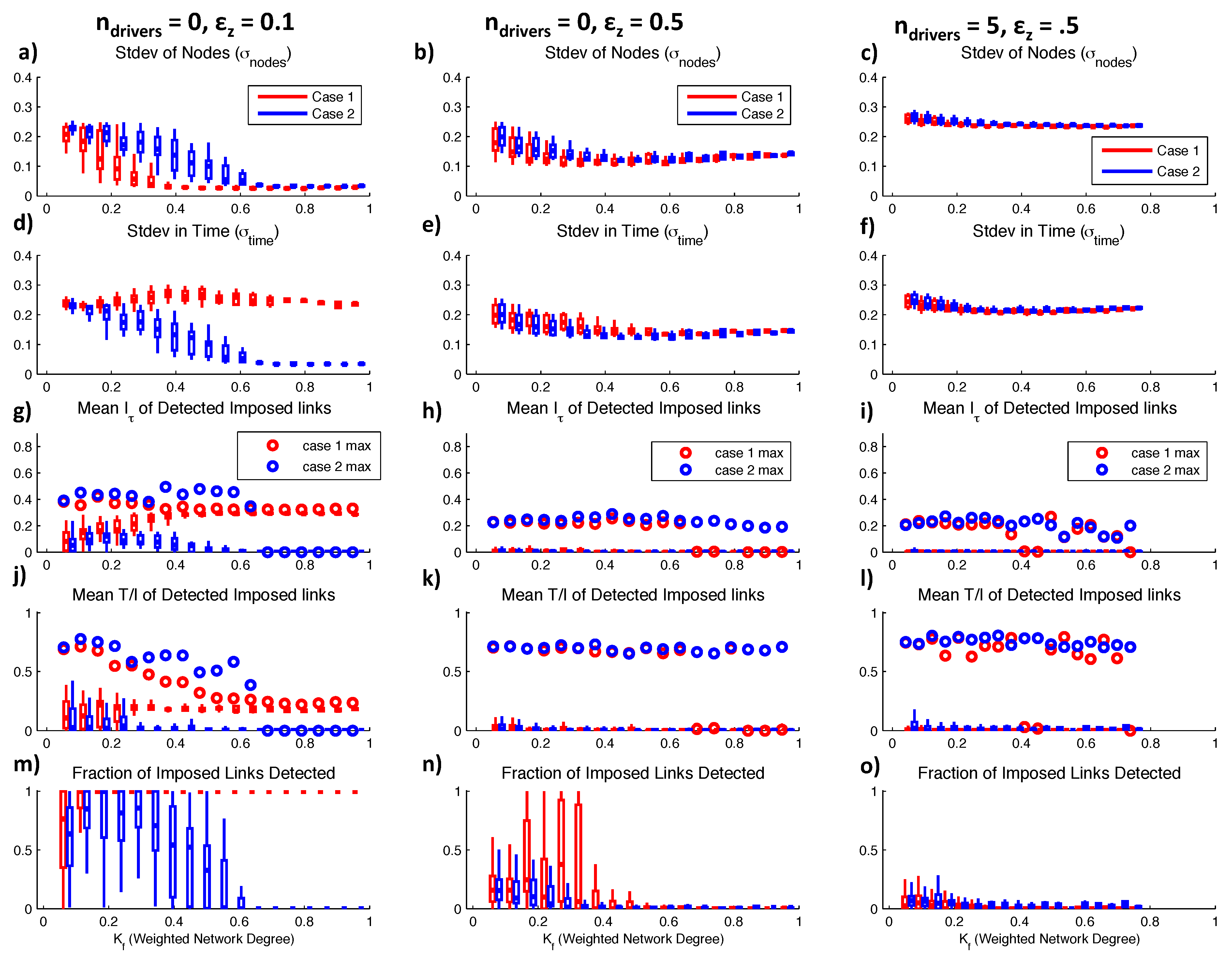
Figure 5. Behaviors of 882 network configurations with range of connectivities $K_f$ for (left) the case with no randomly generated driving nodes, (middle) $n_{drivers}=1$, and (right) $n_{drivers}=5$. (a–c) Standard deviation across nodes ${\sigma }_{nodes}$; (d–f) Standard deviation across time ${\sigma }_{time}$; (g–i) Box plots show mean $I_{\tau }$ detected for all imposed linkages for all networks in each $K_f$ range, and open circles are maximum detected $I_{\tau }$ of any imposed link; (j–l) mean $T/I$ over all networks and maximum detected $T/I$ as in (g–i); (m–o) Fraction of all imposed links that were correctly identified as time dependencies through detected $I_{\tau }$.

Figure 5. Behaviors of 882 network configurations with range of connectivities $K_f$ for (left) the case with no randomly generated driving nodes, (middle) $n_{drivers}=1$, and (right) $n_{drivers}=5$. (a–c) Standard deviation across nodes ${\sigma }_{nodes}$; (d–f) Standard deviation across time ${\sigma }_{time}$; (g–i) Box plots show mean $I_{\tau }$ detected for all imposed linkages for all networks in each $K_f$ range, and open circles are maximum detected $I_{\tau }$ of any imposed link; (j–l) mean $T/I$ over all networks and maximum detected $T/I$ as in (g–i); (m–o) Fraction of all imposed links that were correctly identified as time dependencies through detected $I_{\tau }$.

The mean values of $I_{\tau }$ and $T/I$ displayed in the bar plots of Figure 5g,j represent the mean statistics for imposed links over all networks in each $K_f$ interval, while the maximum $I_{\tau }$ and $T/I$ values displayed in the open circles represent the maximum individual values detected within any of the networks in each $K_f$ range. In other words, mean values represent average detections for imposed links, while the maximum represents overall maximum detected values. For Case 1, mean $I_{\tau }$ for imposed links approaches a constant and statistically significant value of approximately $I_{\tau }=0.25$ (Figure 5g) as the network synchronizes, indicating that the synchronized trajectory retains the imposed uniform $\tau =1$ time dependency. $T/I$ also reaches a constant non-zero value when the network synchronizes, indicating that multiple sources are detected, but the imposed lag is dominant compared to others. For unsynchronized networks ($K_f<0.4$), the low value of mean $T/I$ indicates that most target nodes have multiple sources that lead to redundancies. These redundant sources may not be imposed links from the adjacency matrix, but arise due to induced feedback as illustrated in the two-node example cases. However, for low $K_f<0.2$ in Case 1, we see high maximum individual values of $T/I$ (open red circles in Figure 5j). These high maximum values result from cases in which a target node receives from one source (its own history in the unconnected chaotic logistic case) very strongly, and other sources very weakly, so that $T/I$ is close to 1. Maximum values of $I_{\tau }$ and $T/I$ that are much higher than average values indicate that most imposed links become redundant, but there is at least one less connected node that receives more unique information. For Case 1, $I_{\tau }$ links are weaker on average for less synchronized networks, and more redundant. However, maximum individual $I_{\tau }$ and $T/I$ values are highest for less synchronized networks, representing cases of high coupling strength but low link probability ($ϵ=1$ and $p\ll 1$) in which a single node is a dominant influence on a target.

For Case 2, slightly lower $I_{\tau }$ values are detected for the range of connectivities (Figure 5g). However, we observe very high maximum individual $I_{\tau }$ values over the non-synchronized high connectivity range ($0.5<K_f<0.8$). From the time series (Figure 4b), we see that this is because nodes are generally phase-locked at a time lag of 2 in this range of $K_f$ values, so they are completely predictable based on their own histories. As expected, these high $I_{\tau }$ values are associated with lower $T/I$ (Figure 5j) because of many redundant sources. At complete synchronization ($K_f>0.8$) for Case 2 networks, we see that no $I_{\tau }$ or $T/I$ are detected on average. Case 1 and Case 2 networks show similar behavior at low connectivities, but information measures diverge for the different types of synchronization. $T/I$ decreases as Case 2 networks synchronize, indicating the increase in redundant links. In contrast, $T/I$ increases as Case 1 networks synchronize due to the dominant $(t-1)$ “self”-dependency that arises on the path to synchronization.

We define a correctly detected link as a statistically significant value of $I_{\tau }$ detected for a node pair $(X_i,X_j)$ at the imposed lag time ${\tau }_{j,i}$. For unsynchronized networks with mid-range connectivities ($0.1<K_f<0.6$), we correctly identify nearly all imposed links according to ${\tau }_{i,j}$ for both network cases (Figure 5m). Even for very low-connectivity networks, over half of imposed links are detected. When Case 1 networks are synchronized, a link is detected between every node pair due to the common trajectory, regardless of the imposed w. This leads to a 100% correct link detection rate, but also a 100% “false” detection [37] rate of unimposed links. As discussed in the two-node examples, these detections are all due to induced feedback, thus we do not show their increasing number as networks synchronize. For Case 2, as networks synchronize to a very low amplitude phase-locked state, we cease to detect any of the imposed links.

4.3. Influence and Detection of External Drivers

When nodes in a process network contain complete predictive information, as in the previously discussed noiseless case, complete synchronization occurs at high connectivities. However, real process networks are likely to involve some proportion of nodes that are unpredictable due to influences from outside of the network. These unpredictable nodes may act only as drivers and do not respond to the network dynamics. To simulate these conditions, we generate networks in which one or more nodes ($n_{drivers}$ of N total nodes) have independent dynamics, and act only as sources. While chaotic logistic nodes approach synchronization with increasing $K_f$, the random driving nodes remain independent of this behavior. However, even chaotic logistic nodes do not entirely synchronize due to their varying dependencies on the drivers (Figure 6). From observation of ${\sigma }_{nodes}$ and ${\sigma }_{time}$ for the $n_{drivers}=1$ case (Figure 5b,e), we see similar trends as in the $n_{drivers}=0$ case, but no complete synchronization.

Figure 6. Time series (50 time steps shown) for several generated networks with $n_{drivers}=1$ for (a) Case 1 (b) Case 2.

Figure 6. Time series (50 time steps shown) for several generated networks with $n_{drivers}=1$ for (a) Case 1 (b) Case 2.

For Case 1, we detect similar mean and maximum $I_{\tau }$ values for imposed links over the $K_f$ range (Figure 5h), but maximum $T/I$ values decrease as $K_f$ increases (Figure 5k). This indicates that imposed sources become increasingly redundant with other sources as connectivity increases, and that imposed sources are weaker than induced feedback that arises as the non-driving nodes partially synchronize. The decreasing maximum $T/I$ behavior for Case 1 networks with $n_{drivers}=1$ is very similar to the Case 2 networks with $n_{drivers}=0$. When Case 1 networks are prevented from completely synchronizing due to a random driver, no single source becomes dominant as in the case where $n_{drivers}=0$. Case 2 networks with $n_{drivers}=1$ have lower detected mean and maximum $I_{\tau }$ (Figure 5h) than the $n_{drivers}=0$ case, and lower mean $T/I$ (Figure 5k). However, the maximum individual $T/I$ values are higher at higher $K_f$ values for Case 2, reflecting the influence of the random driving node. If a random driver forces a target node, the shared information is not redundant with any other source, except in the case where induced feedback exists to form an indirect link. For example, if the random node forces an intermediate node that in turn forces the target node, some of the information shared between the the random and target node is also encoded in the intermediate node history, resulting in some redundancy. However, random sources do not propagate feedback as do time-dependent drivers, leading to more unique transfers of information.

When $n_{drivers}=5$, we observe a continuing trend of decreased synchronization capacity (Figure 5c,f), decreased shared information $I_{\tau }$ (Figure 5i), decreased average $T/I$, and increased maximum individual $T/I$ (Figure 5l). We also see that the fraction of correctly detected imposed links decreases with increased randomness in the network (Figure 5m,n,o). For the set of $n_{drivers}=5$ networks, uniform and random τ-distribution cases are nearly indistinguishable, and only slight synchronization is observable from σ measures (Figure 5c,f). Although target nodes receive from a similar number of source nodes as in previous cases, the randomness of some of the sources results in high values of $T/I$, reflecting unique contributions of information. Essentially, any given source node may only share a small amount of information with a target node, but this information is more likely to be unique if the source is random. On average however, linkages are increasingly redundant (low $T/I$) as connectivity increases and feedback is created.

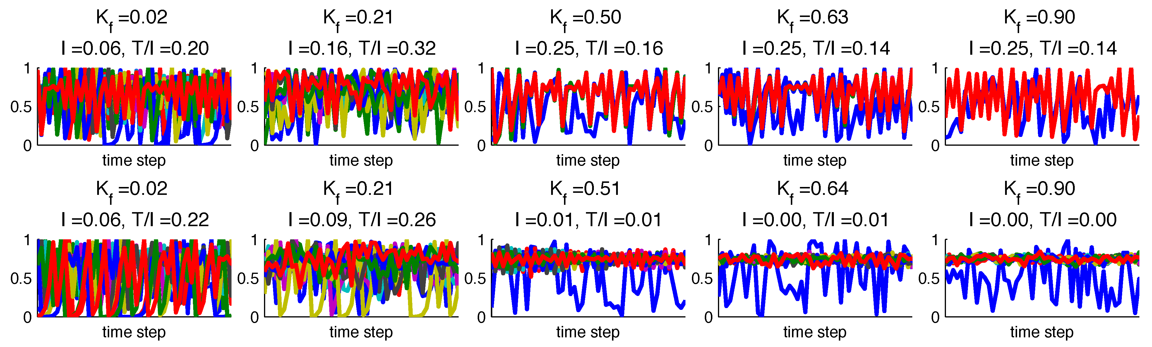
4.4. Influence of Noise in Network

In real networks, variability cannot always be attributed to the behavior of other nodes, but may be caused by noise. In this section, we set ${ϵ}_z>0$ in Equation (18) to represent sources of variability such as measurement noise. While randomly generated driving nodes force other network components according to connectivity as determined by adjacency matrix w, a noise component represents random variability z applied to each node. Similar to cases where $n_{drivers}>0$, randomness due to ${ϵ}_z>0$ prevents complete synchronization. The introduction of noise as 10% of the coupling strength (${ϵ}_z=0.1$) to the case with no random drivers (Figure 7 Left) results in similar synchronization behavior as the initial noiseless scenario (Figure 5 Left), except that nodes do not completely synchronize. In contrast to the $n_{drivers}>0$ cases, all nodes contain time dependencies in addition to the noise components, and we observe that nodes tend to synchronize to an equal degree (Figure 8) as $K_f$ increases. When the noise component is increased to ${ϵ}_z=0.5$, the network further loses capacity to synchronize (Figure 7b,e), and Cases 1 and 2 are nearly indistinguishable.

The shared information $I_{\tau }$ for the ${ϵ}_z=0.1$ case (Figure 7g) is similar to the initial noiseless case (Figure 5g) for Case 1 networks, but lower for Case 2 networks. While mean detected $I_{\tau }$ increases with $K_f$ for Case 1 networks up to a constant value, we observe an opposite trend in $T/I$, in which the maximum detected $T/I$ decreases with increased $K_f$ until it reaches a constant low value at $K_f=0.6$. As the nodes partially synchronize, the noise components cause scatter in the $pdf$s that results in similar strengths of information measures between sources. The detected $T/I$ is similar to the case with 1 external driver (Figure 7k). At low $K_f$, a node may receive a large amount of unique information from a source, but feedback results in redundancy at high $K_f$.

Figure 7. Behaviors of 882 network configurations with range of connectivities $K_f$ for (left) $n_{drivers}=0$ and ${ϵ}_z=0.1$, (middle) $n_{drivers}=0$ and ${ϵ}_z=0.5$, and (right) $n_{drivers}=5$ and ${ϵ}_z=0.5$ (a–c) Standard deviation of nodes; (d–f) Standard deviation in time; (g–i) Box plots indicate mean $I_{\tau }$, and open circles are maximum detected $I_{\tau }$; (j–l) mean and maximum detected $T/I$ values as in (g–i); (m–o) Fraction of all imposed links that were correctly identified as peak time dependencies through detected $I_{\tau }$.

Figure 7. Behaviors of 882 network configurations with range of connectivities $K_f$ for (left) $n_{drivers}=0$ and ${ϵ}_z=0.1$, (middle) $n_{drivers}=0$ and ${ϵ}_z=0.5$, and (right) $n_{drivers}=5$ and ${ϵ}_z=0.5$ (a–c) Standard deviation of nodes; (d–f) Standard deviation in time; (g–i) Box plots indicate mean $I_{\tau }$, and open circles are maximum detected $I_{\tau }$; (j–l) mean and maximum detected $T/I$ values as in (g–i); (m–o) Fraction of all imposed links that were correctly identified as peak time dependencies through detected $I_{\tau }$.

Figure 8. Time series (50 time steps shown) for several generated networks with ${ϵ}_z=0.1$ and no random driving nodes for (a) Case 1 (b) Case 2.

Figure 8. Time series (50 time steps shown) for several generated networks with ${ϵ}_z=0.1$ and no random driving nodes for (a) Case 1 (b) Case 2.

Increasing the noise component to ${ϵ}_z=0.5$ (Figure 7b,e) results in similar ${\sigma }_{nodes}$ and ${\sigma }_{time}$ as the $n_{drivers}=5$ case, in which the two cases are not distinguishable. However, the mean $I_{\tau }$ and $T/I$ (Figure 7h,k) are very small compared to the case with random driving nodes. For Case 1, there is a threshold connectivity value around $K_f=0.7$ at which no $I_{\tau }$ is detected for any imposed link. This is due to the high noise in addition to many source nodes. Nodes would synchronize to a chaotic trajectory if not for the noise, and the spread of the resulting $pdf$ does not allow for significant detection of any sources. For Case 2, maximum detected $I_{\tau }$ is statistically significant even at high $K_f(>0.7)$ values, because nodes tend toward synchronization to a phase-locked trajectory in which $X_i\left(t\right)=X_i(t-2)$. Although $T/I$ is very low on average for ${ϵ}_z=0.5$ networks (Figure 7k), the maximum detected $T/I$ is high over the range of connectivities. Similar to the case of multiple random drivers, when a target node receives from a single source that is partially random, the information due to the random component is more likely to be unique, resulting in a high $T/I$.

A final case in which $n_{drivers}=5$ and ${ϵ}_z=0.5$ combines the influences of random driving nodes and noise. In this case, little synchronization is detected based on σ measures (Figure 7c,f) for either Cases 1 or 2. Shared information $I_{\tau }$ is statistically significant over the range of $K_f$, but very small (Figure 7i). However, the maximum individual $T/I$ values tend to be large over the entire $K_f$ range, similar to the previous cases with high noise levels in the form of either random drivers or noise.

As noise and randomness are introduced in the networks, fewer imposed links are correctly identified (Figure 7m,n,o). However, for high $K_f>0.5$, a higher fraction of imposed links is detected in the case with random drivers and noise (Figure 7o) than the case with only noise (Figure 7n). This is because the random drivers transmit information more strongly than source nodes composed of both noise and chaotic logistic components, so are more likely to be detected at higher $K_f$ values. Detection of links improves with longer time series datasets, but we consider only networks of $n=200$ data points to reflect realistic data availability. For all of the network cases generated, some links are not detected at low $K_f$ values because they are very weak. At high $K_f$, links other than those imposed are detected due to feedback induced by the high connectivity.

4.5. Summary of Structure and Synchronization of Networks

The addition of randomness or noise to a connected network prevents complete synchronization. This random component could be in the form of driving nodes that do not directly participate in feedback, or in the form of noise inherent to each individual node. Driving nodes remain independent of the synchronization of the rest of the network, while nodes in a noisy but feedback-connected network synchronize to an equal degree. Measures of ${\sigma }_{nodes}$ and ${\sigma }_{time}$ are useful to gage the relative level of synchronization, and particularly distinguish between uniform and random delay τ-distributions in noiseless network cases through their detection of synchronization and amplitude death. However, they do not convey information about time dependencies and redundancies within the network, and do not distinguish between high and low connectivities when there is a high level of randomness.

Information measures such as lagged mutual information ($I(X_{tar};X_{s1})$), conditional information given other sources ($I(X_{tar};X_{s1}|X_{s2})$), and total shared information between multiple sources ($I(X_{tar};X_{s1},X_{s2})$) detect time dependencies between node pairs in a process network, and enable detection of dominant drivers, and unique and redundant sources of information. Even for completely synchronized nodes, $I_{\tau }$ detects time dependencies within a single trajectory, as in the noiseless Case 1 (uniform τ-distribution) networks. For unsynchronized networks with detected time dependencies (significant $I_{\tau }$), $T/I$ further conditions on other source nodes and time scales to reveal redundancies and unique links. A $T/I>0$ indicates that the detected link is not completely redundant given the history of another source node, which could be the target’s own history, as is detected with transfer entropy. In the case of a network forced only by feedback, there may be high $I_{\tau }$ between node pairs, but low $T/I$ due to redundancies in the synchronizing nodes. In contrast, for a network forced randomly or by a node with no time dependencies, target nodes may share information with only one source, or completely unique sources. In these cases, we detect both significant $I_{\tau }$ and $T/I$, indicating a high level of unique information transfer.

We define a correctly detected link as statistically significant value of lagged mutual information $I_{\tau }$ detected between two nodes ($X_i,X_j$) that corresponds to an imposed link according to $w_{i,j}$ and ${\tau }_{i,j}$. In a weakly connected network with little noise, we identify nearly all imposed links. As connectivity increases, if nodes tend to synchronize to a time-dependent trajectory, we increasingly detect “false” links between nodes that are not defined to be connected, or are connected at a different time scale. These false links are actually feedback induced by the imposed time dependencies. When a network begins to synchronize, it is not possible to distinguish links due to imposed network structure from those due to induced feedback. In cases where nodes synchronize to a fixed point trajectory, we cease to detect any links. In networks with noise, some imposed links are correctly detected at high levels of connectivity since the random components provide unique information that prevents complete synchronization.

5. Discussion

The two-node and 10-node network scenarios presented here represent a small fraction of potential network dynamics that could be observed in real-world networks. The two-node networks help us understand induced feedback and types of forcing, and the resulting interpretation from analysis of the data. The 10-node networks capture general features of a larger network dynamic arising from multiple pieces of feedback. Process networks based on measured or simulated nodes of time series exhibit a wide range of connectivities and time-varying interactions. Coupling strengths and timescales vary between nodes and shift over time, and thresholds may exist for which certain couplings break down while others become dominant. Additionally, shared information between two or more variables could be synergistic, if the knowledge of two nodes together provides more information than their union separately. Although we present relatively simple cases in this study, the metrics used for analysis allow for the detection of a range of behaviors such as complete or partial synchronization, weak or strong time dependencies, and redundancy or uniqueness of shared information. The information theoretic measures used in this study may be compared with efficient statistical learning methods applied to graphical models, such as the graphical lasso [13] or methods that combine graphical models with conditional dependencies [14], particularly in cases with many time series nodes.

In real-world process networks in which noise and other drivers prevent complete synchronization, some detected time dependencies are likely to correspond to causality (i.e., “correctly detected links”), while others represent induced feedback. When nodes in the network are highly connected with feedback present, detected links are identified as redundant, and it is difficult to distinguish critical interactions from induced feedback. This feature of process networks indicates a future challenge in terms of connecting network time dependencies to system functionality.

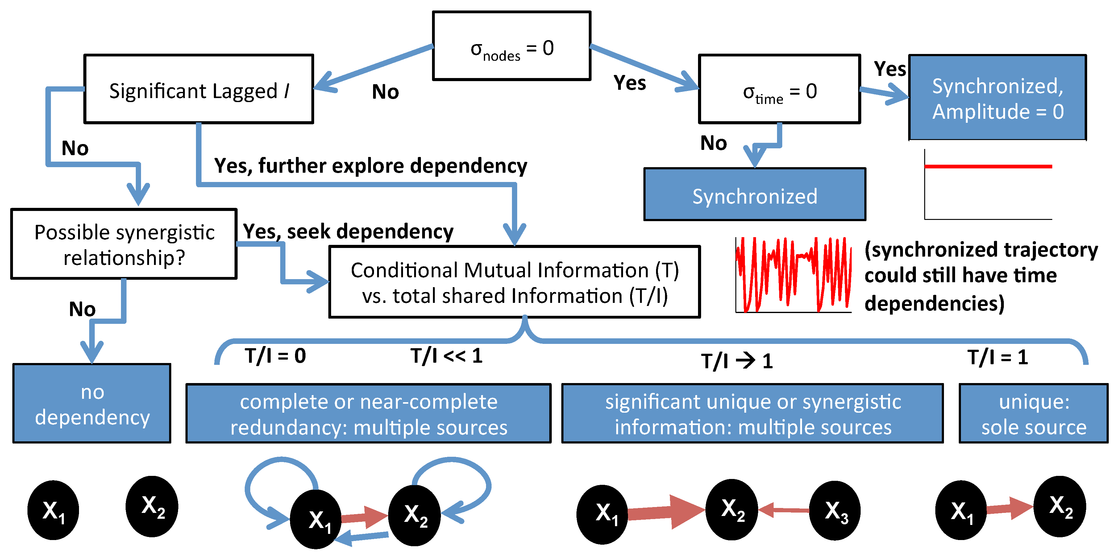
Figure 9 categorizes the range of possible whole-network or subsystem behaviors that can be extended to an observed process network. If a network is not completely synchronized, nodes could be lag-synchronized, or transferring and receiving information at different time scales and strengths. Real-world process networks consist of measured time-series data for which the underlying mechanisms are partially or completely unknown. There may be unmeasured or hidden driving and receiving nodes, and network connectivity can shift over time. The weakening of a single link may result in decreased redundancy in the form of induced feedback throughout an entire network. For real process network analysis, the measures presented in this study can aid in comparing observations to simulation results, evaluating system states, or assessing the influence of noise or bias on time dependencies.

Figure 9. Illustration of a range of network dynamics that can be identified using information theoretical measures. Nodes are synchronized if ${\sigma }_{nodes}=0$ and synchronized to zero-amplitude trajectories if ${\sigma }_{time}=0$. In asynchronous cases, the absence of statistically significant $I_{\tau }$ indicates a disconnected network in the case of no synergistic shared information. Otherwise, the dependencies between nodes can be further explored with conditional and total information measures ($T/I$). If $T/I=0$, multiple sources are completely redundant with each other. If $T/I=1$, there is only 1 unique source providing information to the target node. In between, sources can be partially redundant, synergistic or unique.

Figure 9. Illustration of a range of network dynamics that can be identified using information theoretical measures. Nodes are synchronized if ${\sigma }_{nodes}=0$ and synchronized to zero-amplitude trajectories if ${\sigma }_{time}=0$. In asynchronous cases, the absence of statistically significant $I_{\tau }$ indicates a disconnected network in the case of no synergistic shared information. Otherwise, the dependencies between nodes can be further explored with conditional and total information measures ($T/I$). If $T/I=0$, multiple sources are completely redundant with each other. If $T/I=1$, there is only 1 unique source providing information to the target node. In between, sources can be partially redundant, synergistic or unique.