Response of Surface Ultraviolet and Visible Radiation to Stratospheric SO2 Injections
by
 , and
, and
Sasha Madronich
1,* ,
,
Simone Tilmes
1,
Ben Kravitz
2,
Douglas G. MacMartin
3 and
Jadwiga H. Richter
4 1
Atmospheric Chemistry, Observations, and Modeling Laboratory, National Center for Atmospheric Research, Boulder, CO 80307, USA
2
Atmospheric Sciences and Global Change Division, Pacific Northwest National Laboratory, Richland, WA 99352, USA
3
Mechanical and Aerospace Engineering, Cornell University, Ithaca, NY 14853, USA
4
Climate and Global Dynamics Laboratory, National Center for Atmospheric Research, Boulder, CO 80307, USA
*
Author to whom correspondence should be addressed.
Atmosphere 2018, 9(11), 432; https://doi.org/10.3390/atmos9110432
Submission received: 17 August 2018
/
Revised: 30 October 2018
/
Accepted: 2 November 2018
/
Published: 7 November 2018
(This article belongs to the Special Issue Radiative Transfer in the Earth Atmosphere)
Abstract
:Climate modification by stratospheric SO2 injections, to form sulfate aerosols, may alter the spectral and angular distributions of the solar ultraviolet and visible radiation that reach the Earth’s surface, with potential consequences to environmental photobiology and photochemistry. We used modeling results from the CESM1(WACCM) stratospheric aerosol geoengineering large ensemble (GLENS) project, following the RCP8.5 emission scenario, and one geoengineering experiment with SO2 injections in the stratosphere, designed to keep surface temperatures at 2020 levels. Zonally and monthly averaged vertical profiles of O3, SO2, and sulfate aerosols, at 30 N and 70 N, served as input into a radiative transfer model, to compute biologically active irradiances for DNA damage (iDNA), UV index (UVI), photosynthetically active radiation (PAR), and two key tropospheric photodissociation coefficients (jO1D for O3 + hν (λ < 330 nm) → O(1D) + O2; and jNO2 for NO2 + hν (λ < 420 nm) → O(3P) + NO). We show that the geoengineering scenario is accompanied by substantial reductions in UV radiation. For example, comparing March 2080 to March 2020, iDNA decreased by 25% to 29% in the subtropics (30 N) and by 26% to 33% in the polar regions (70 N); UVI decreased by 19% to 20% at 30 N and 23% to 26% at 70 N; and jO1D decreased by 22% to 24% at 30 N and 35% to 40% at 70 N, with comparable contributions from sulfate scattering and stratospheric O3 recovery. Different responses were found for processes that depend on longer UV and visible wavelengths, as these are minimally affected by ozone; PAR and jNO2 were only slightly lower (9–12%) at 30 N, but much lower at 70 N (35–40%). Similar reductions were estimated for other months (June, September, and December). Large increases in the PAR diffuse-direct ratio occurred in agreement with previous studies. Absorption by SO2 gas had a small (~1%) effect on jO1D, iDNA, and UVI, and no effect on jNO2 and PAR.
1. Introduction
The surface temperature of Earth has been increasing in the past half-century at a rate that is unparalleled beyond human history, even over ice-core records extending back hundreds of thousands of years [1]. Potential strategies for reducing this global warming include the injection of sulfur dioxide gas (SO2) into the stratosphere, where, within a few weeks, it would be converted to sulfate particles and thus reduce the transmission of solar radiation to the surface [2,3,4]. However, such injections could cause many other changes in the atmosphere and over terrestrial and aquatic ecosystems. These include changes in circulation, cloud cover, precipitation, as well as in the stratospheric ozone (O3) [5,6,7,8,9], with details being sensitive to the timing, location, and amount of SO2 injections, as well as the model configuration and future scenarios [6,10,11]. Perturbations to optically active constituents of the atmosphere (SO2, O3, and sulfate aerosols) can affect not only the average total radiation, but also some more detailed aspects, such as its wavelength distribution, direct-diffuse ratios, and changes in its daily and seasonal cycles. Given the central role that solar radiation plays in a multitude of photochemical and photobiological processes at or near the planet’s surface, comprehensive evaluations of the possible systematic changes are necessary.
The effects of sulfate aerosols on the atmospheric radiation field, from the SO2 injected into the stratosphere by the eruptions of El Chichon and Mt. Pinatubo, were simulated by Michelangeli et al. [12,13] and were shown to be complex, with both reductions and enhancements of ultraviolet (UV) irradiances transmitted to the troposphere. Reductions occur mainly by aerosols attenuating the direct solar beam, while enhancements can result from both multiple scattering (photon trapping), between the aerosols and the Rayleigh atmosphere, and by single scattering from stratospheric aerosols, providing optical shortcuts through the O3 column below it [13,14,15]. The interactions between aerosol scattering and O3 absorption are particularly important in the UV-B band (280–315 nm), for which the O3 column is the main determinant of the total optical depth. Vogelman et al. [16] concluded that depletion of O3 itself, by heterogeneous chemistry on sulfate aerosols, more than offset any UV reductions that were caused due to aerosols. Scattering by aerosols can also increase the diffuse irradiance (sky radiation) while attenuating the direct beam. Large increases in the diffuse-direct irradiance ratios were observed after the Mt. Pinatubo eruption at both UV [17] and visible [18] wavelengths, and are expected in sulfate geoengineering scenarios [19,20], as discussed by Xia et al. [21]. More recently, Eastham et al. [22] examined the effect of sulfate geoengineering on mortality associated with air quality (UV and temperature effects on ground-level O3 and particulate matter (PM)) and skin cancer.
Here, we focus on changes in surface UV and visible radiation, under a proposed geoengineering scenario that is designed [10] to keep surface temperatures at 2020 values, despite increasing greenhouse gas concentrations, following the Representative Concentration Pathway 8.5 (RCP8.5), the worst case considered by the Intergovernmental Panel on Climate Change (IPCC) [1]. We consider the effects on several important but different photo-processes that illustrate dependencies on both wavelength and diffuse-direct ratios, these include: The UV irradiances that damage DNA and skin, the UV actinic fluxes that drive tropospheric photochemistry, and visible photosynthetically active radiation (PAR). Results for 2080, from simulations with and without geoengineering, are compared to 2020 at two latitudes, 30 N and 70 N, and for four months in different seasons, chosen to represent a wide range of prevailing solar zenith angles and other environmental conditions.
2. Methods
2.1. The CESM1(WACCM) Model
The model data for this study were taken from simulations performed with the Community Earth System Model, version 1 (CESM1) [23], using the Whole Atmosphere Community Climate Model (WACCM) as its atmospheric component [24]. CESM1 interactively coupled the atmospheric, land, sea-ice, and ocean components of the Earth’s system. The atmospheric model, WACCM, included comprehensive stratospheric chemistry and a modal aerosol model that were both interactively coupled to radiation and transport. The model included an interactive quasi-biennial oscillation (QBO) and the ability to inject sulfur (SO2) into the stratosphere, which, in a few weeks, would oxidize to form sulfuric acid (H2SO4) that condenses to form sulfate aerosols. Aerosol extinction was computed by Mie scattering theory at 350, 550, and 1020 nm. Biogenic emissions were produced by the Model of Emissions of Gases and Aerosols from Nature (MEGAN), version 2.1 [25]. WACCM does not compute changes in radiation due to stratospheric aerosol loading, and therefore these were calculated off-line below using a radiative transfer model (see Section 2.4). The simulations were performed using a 0.9° latitude × 1.25° longitude horizontal resolution, with 70 vertical layers reaching up to 140 km (~10−6 hPa). Details of the model setup are given by Mills et al. [24] with modifications described by Tilmes et al. [26]. The model has been previously evaluated and, in particular stratospheric ozone and aerosol distributions, showed good agreement with observations for past and present conditions [24].
2.2. Numerical Experiments
We employed simulations performed for the stratospheric aerosol geoengineering large ensemble (GLENS) project using CESM1(WACCM) [26]. The simulations are summarized in Table 1. GLENS simulations included a 20-member ensemble of RCP8.5 simulations between 2010 and 2030, with three of these simulations continued until 2097. They further included a 20-member geoengineering ensemble between 2020 and 2099 [26]. Differences in column ozone due to these setup differences were minor.
The geoengineering simulation was designed to keep global surface temperatures at 2020 values while using the RCP8.5 greenhouse gas scenario between 2020 and 2099. This was achieved by injecting SO2 into the stratosphere at four predefined locations away from the equator, at 15 N, 15 S, 30 N, and 30 S, and at around 5 km above the tropopause. The annual injection amount, starting in 2021 at each of the four locations, was determined by a feedback controller, in order to reach three independent surface temperature goals, namely keeping global temperatures, the interhemispheric temperature gradient, and the temperature gradient between the equator and the pole at 2020 levels. Details of this approach are described by MacMartin et al. [27] and Kravitz et al. [8]. Approximately 40 TgSO2/year by 2080 were required to maintain the three temperature goals.
2.3. Time Periods Considered
Zonal averaged profiles of ozone, SO2, and sulfate extinction at 30 N and 70 N were investigated for two time periods, a current time using the year 2020 and a future time of 2080. The latitudes were selected as roughly representative of the subtropics (30 N), with intense noontime radiation and large daily variation in solar zenith angles (sza), in contrast to polar regions (70 N), where ecosystems that have adapted to low-light levels may be particularly sensitive to increases in UV and visible radiation. We selected the month of March for analyzing typical responses, but also present some results for June, September, and December.
For 2020, we used an average of all the data for that year from the 17-member RCP8.5 ensemble. For 2080, we averaged the data for the available members for either the no-geoengineering RCP8.5 simulations (3 members), or the geoengineering experiment (20 members). The different ensemble memberships stemmed from issues of computational cost, hardware, and stability (for the RCP8.5 simulations), and we recognize that larger ensembles may be desirable in future studies.
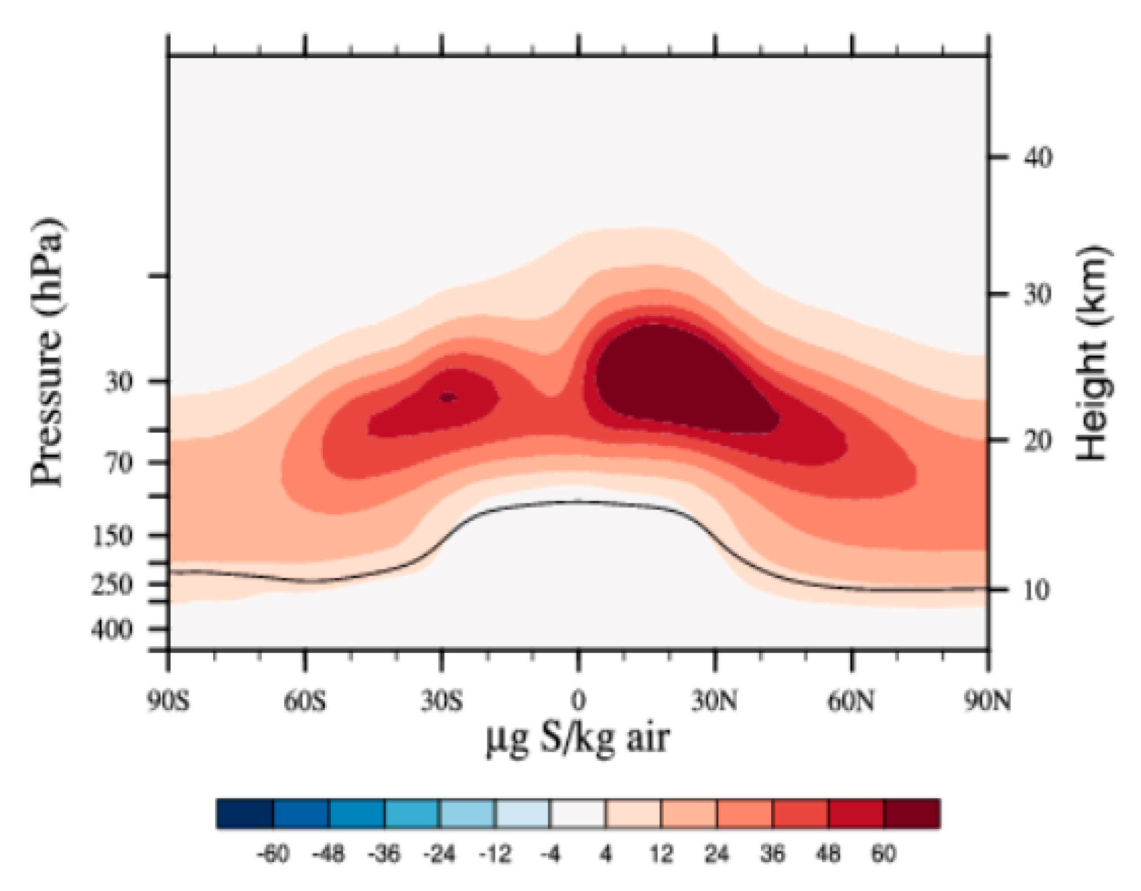
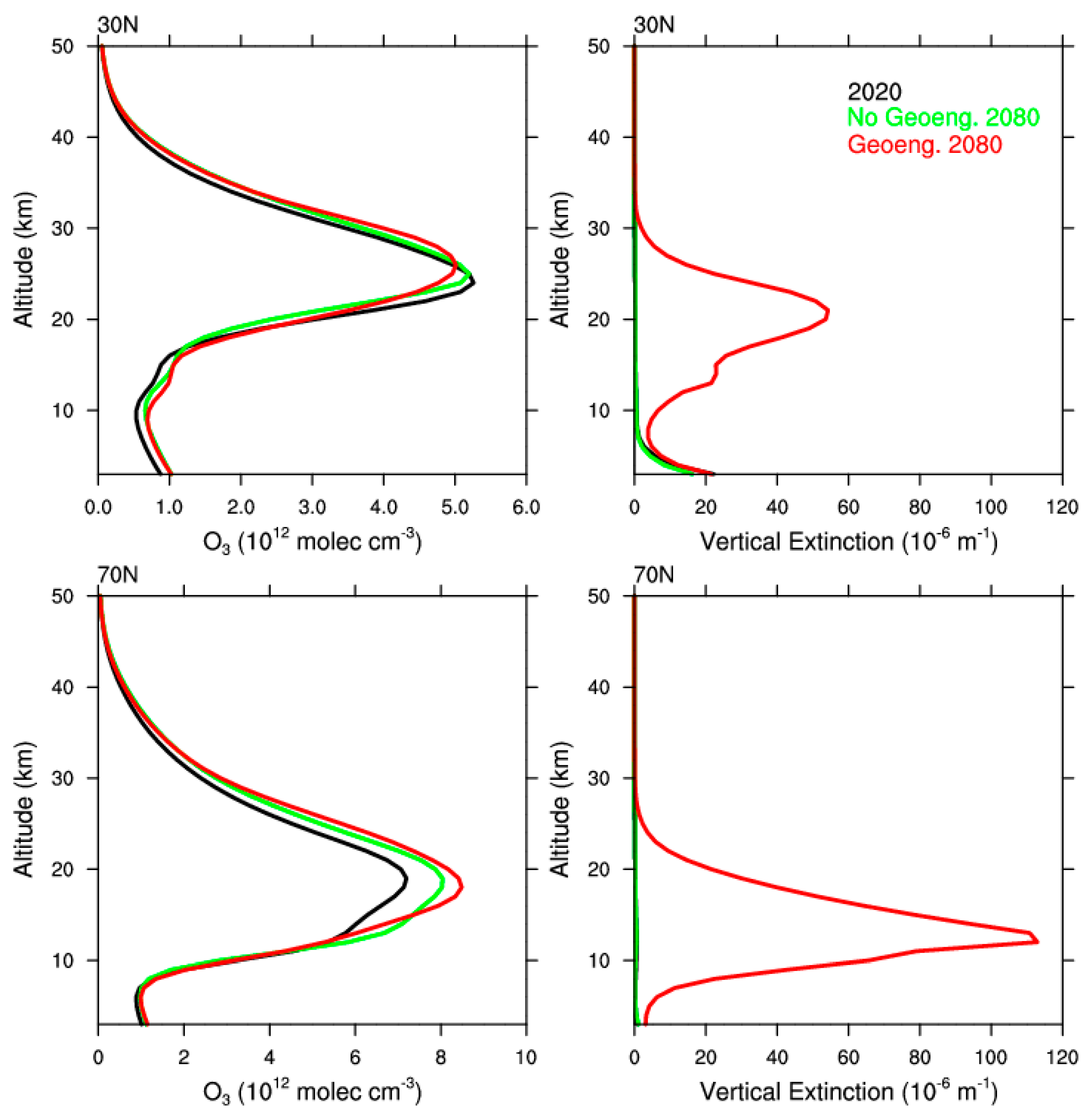
Figure 1 shows stratospheric sulfate aerosol distribution for the geoengineering experiment for March 2080. Injections at altitudes around 5 km above the tropopause resulted in an aerosol distribution that reached above 30 km in the tropics and above 25 km in the high latitudes. Vertical profiles of O3 and sulfate extinction at 30 N and 70 N are shown in Figure 2. Ozone concentrations at 30 N peaked at around 25 km, whereas concentrations at 70 N peaked at around 20 km. In 2080, O3 concentrations increased for both latitudes due to the ozone recovery, from reductions of halogen-induced O3 depletion, and the super-recovery of O3, driven by cooler stratospheric temperatures for a high greenhouse gas emission scenario, which slows down gas-phase ozone destroying cycles (green lines).
In terms of total column ozone, for 30 N a slight increase between 2020 and 2080 was shown (Table 2). For 70 N, column ozone had already recovered by 2040 to 2050, for both RCP8.5 and the geoengineering case, as shown by Richter et al. [9]. For months other than March, the total column amounts of O3, SO2, and sulfate 500 nm extinctions are shown in Figure S1 (Supplementary Materials) and were qualitatively similar to the March values.
2.4. Tropospheric Ultraviolet-Visible (TUV) Model
The vertical composition profiles from the CESM1(WACCM) simulations, described in Section 2.1, Section 2.2 and Section 2.3, were used off-line in the Tropospheric Ultraviolet-Visible (TUV, v.5.3) model, to simulate the propagation of solar radiation through the atmosphere, and thus compute biologically effective irradiances and photo-dissociation coefficients at the Earth’s surface. The TUV model has been described before and evaluated with measurements [28,29,30]. For the present studies, we considered molecular absorption by O3 and SO2, Rayleigh scattering by air molecules, scattering and absorption by aerosols, and a wavelength-independent surface albedo of 10% (options for clouds, snow packs, and gaseous O2 and NO2 were not used). The model aerosols were assumed to be entirely sulfate, with wavelength-independent values for single scattering albedo of 0.99 and asymmetry parameter of 0.71, and vertical extinction profiles computed from CESM1(WACCM) at 350, 550, and 1020 nm. The aerosol extinction was scaled to other wavelengths with a power function λ−α, where α, the Angstrom exponent, was estimated for λ < 550 nm from the extinction at 350 and 550nm, and for λ > 550 nm from the extinction at 550 and 1020 nm. The model values of α tended to be rather small, particularly for UV and visible extinctions, which were seen to be quite comparable (Table 2); a similar behavior was observed for Mt. Pinatubo aerosols after about one year of processing, with very little wavelength dependence between 400 and 1020 nm [31].
For modeling purposes, aerosol scattering was represented by a Henyey-Greenstein phase function, and its moments used as input into a 4-stream discrete ordinates solver, with pseudo-spherical correction for improved accuracy at low sun conditions. Other aerosols (dust, organics, sea-salt, soot, etc.) or clouds, although represented in the CESM1(WACCM) simulations [24], were not considered for the TUV simulations, for simplicity but also because they were highly variable on local scales.
The TUV model computed spectral irradiances and actinic fluxes in 1.0 nm intervals over 280–700 nm, separately tallying the direct solar beam, and the diffuse-sky and reflected radiation. The spectral irradiances and actinic fluxes were multiplied by weighting functions, w(λ), representing either biological sensitivity (action) spectra, B(λ), or molecular product of absorption spectrum, σ(λ), and photodissociation quantum yield, ϕ(λ), then integrated over wavelength:
where F(λ) is either:
(Biologically effective irradiance) or (photo-dissociation coefficient) = ∫λ w(λ) F(λ) dλ
- The spectral irradiance if w(λ) = B(λ), integrated over 2π steradians (downwelling);
- the spectral actinic flux if w(λ) = σ(λ)ϕ(λ), integrated over 4π steradians.
We consider here, two biological weighting functions of broad interest: (1) The standard action spectrum for the induction of erythema (reddening) of human skin by sunlight, which is also used for the computation of the UV index (UVI) that is widely available to the public [32,33]; and (2) the action spectrum for in-vitro damage to DNA molecules [34], which closely follows the absorption cross section of DNA molecules [35]. Both of these biological endpoints show increasing response toward shorter UV wavelengths and are consequently sensitive to the overhead ozone amount, with normalized sensitivity coefficients (% increase in effective radiation for a 1% decrease in O3) of about 1.1 for UV Index and 2.2 for iDNA, the irradiance weighted by the DNA damage spectrum [36].
We also consider here two photo-dissociation reactions that are fundamental in tropospheric chemistry:
O3 + hν (λ < 330 nm) → O(1D) + O2 jO1D
NO2 + hν (λ < 420 nm) → O(3P) + NO jNO2
2.5. Reductions and Enhancements of Surface UV-B by a Single Aerosol Layer
Scattering of sunlight by stratospheric aerosols is generally expected to decrease the solar irradiance reaching the surface at most wavelengths, but an interesting exception occurs in the UV-B range. Strong absorption by O3 greatly limits the transmission of UV-B, especially at large solar zenith angles (low sun), when the optical path through O3 becomes increasingly long. Sulfate aerosols can change these optical paths, and can theoretically enhance (or reduce) the UV-B transmission depending on their vertical placement relative to the O3 layers. Although this enhancement has been noted before [12,13,14,15], we re-examined it here because of its potential importance in low sun environments (e.g., high latitude regions). To gain insight into this coupling, we started with the aerosol-free U.S. Standard Atmosphere [39] and added a hypothetical single aerosol layer, 1 km thick, to it, with an optical depth of 0.2, and then computed the changes in surface UV-B irradiance; this was repeated at each altitude, and for several different solar zenith angles, with results shown in Figure 3. Aerosols added in the lower atmosphere (0–10 km) simply reduced surface DNA-damaging radiation. However, when aerosols were added in or above the peak O3 altitudes (ca. 20–25 km), significant enhancements in surface radiation could occur at the shortest wavelengths, if photons scattered toward the nadir encountered a shorter optical path through the O3 below. The effect was not monotonic with solar zenith angle (sza), but showed a sharp maximum for sza, near 80 ± 5°. For a smaller sza, sulfate scattering provided only relatively minor reductions in the O3 optical paths, or even increased them. For very low sun, the direct beam no longer reached the ground, but was the source of scattering (Rayleigh from air molecules and Mie from sulfate aerosols) that constituted the main remaining source of UV-B irradiance reaching the surface.
Another important consideration is the asymmetry factor, g, of the aerosols, which determines the fraction of downward scattered radiation. While here we used g = 0.71 [31], in a separate sensitivity study, using g = 0.60 resulted in somewhat greater transmission at lower sza, generally increasing the importance of this effect.
In the tropics and mid-latitudes, this sza = 80 ± 5° window is encountered only briefly, twice per day, but in polar regions the sun can be hovering at those angles for many hours and even days. For example, at the North Pole the sza remains between 75% to 85° for about 50 days, from 2 April to 1 May, and again from 12 August to 10 September, the latter time period coinciding with the annual minimum in sea-ice, thus exposure is potentially increased for vulnerable Arctic marine [40] and terrestrial [41] ecosystems. It remains to be seen, below, to what extent such enhancements are possible with realistic SO2 injection heights and resultant sulfate vertical distribution.
3. Results
3.1. Diurnal Cycles of Biologically Active Radiation
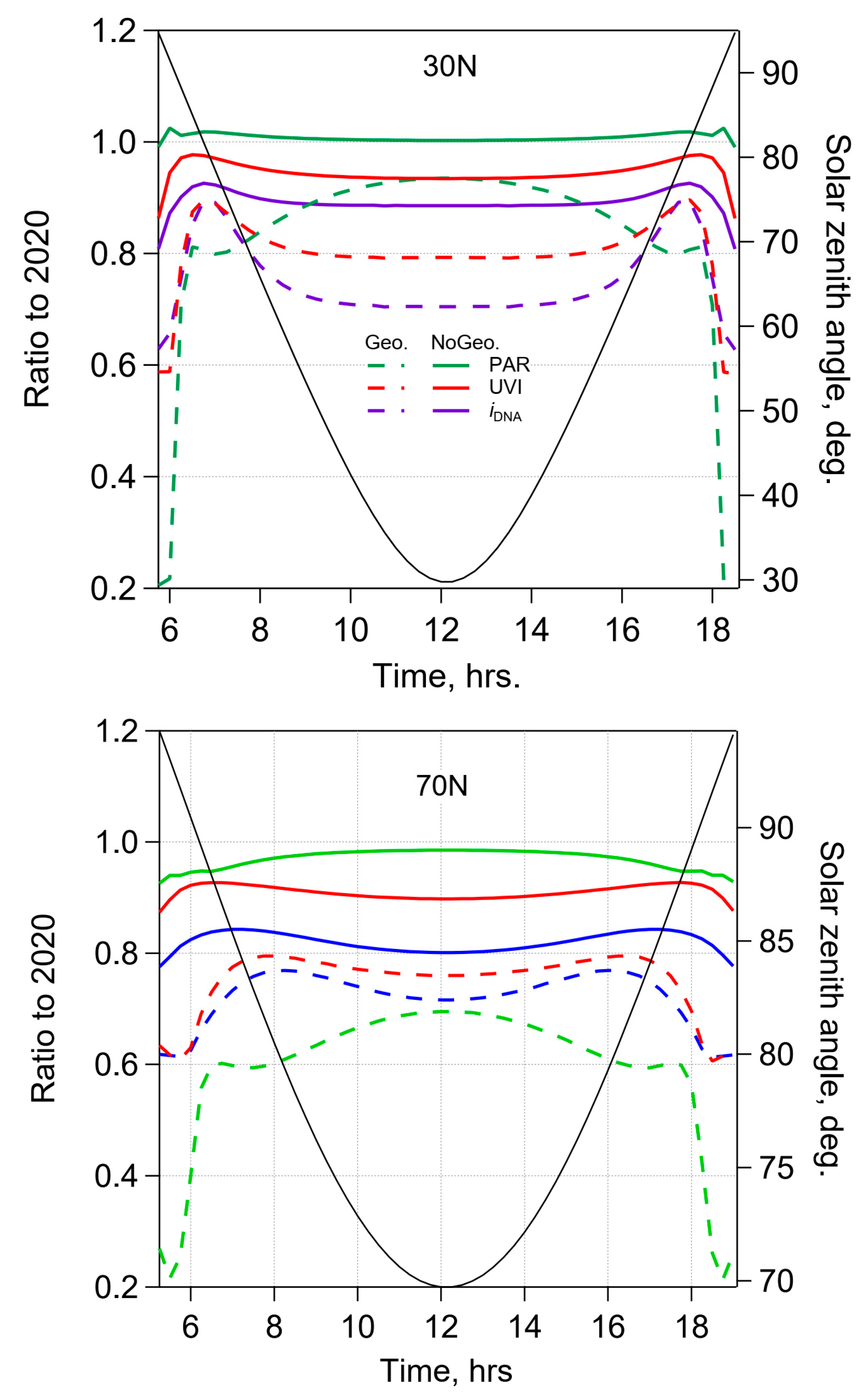
We next consider the radiative effects of the vertical distributions of aerosols and ozone, predicted by the CESM1(WACCM) model under different scenarios. Figure 4 shows the scenario changes for several biological effects (iDNA, UVI, and PAR) relative to current day (2020). In the scenario without geoengineering, PAR was essentially unaffected, wheres some reductions were seen for the UVI and iDNA due to the recovery of stratospheric O3. With geoengineering, UVI and iDNA were reduced by an additional 10% to 20%, whereas for PAR the reductions ranged from 10% at 30 N to nearly 40% at 70 N. Contrary to the results with an idealized single layer of sulfate (Figure 3), UVI and iDNA were not enhanced at any sza, but did show a relative increase in transmission when the sza was near 80°; most evident in Figure 4 as a “shoulder”, seen at 30 N in the early morning and late afternoon. At 70 N, this effect was less pronounced, mainly because the sza remained in the 70–90° range throughout the daylight hours, but was manifest as a smaller difference between UVI and iDNA reductions. Thus, while the sulfate-derived increased transmission for sza near 80° did not give a net enhancement of surface UV irradiances, the reductions by the coupled sulfate-O3 system were smaller than expected if sulfate extinction and O3 absorption were considered independently.
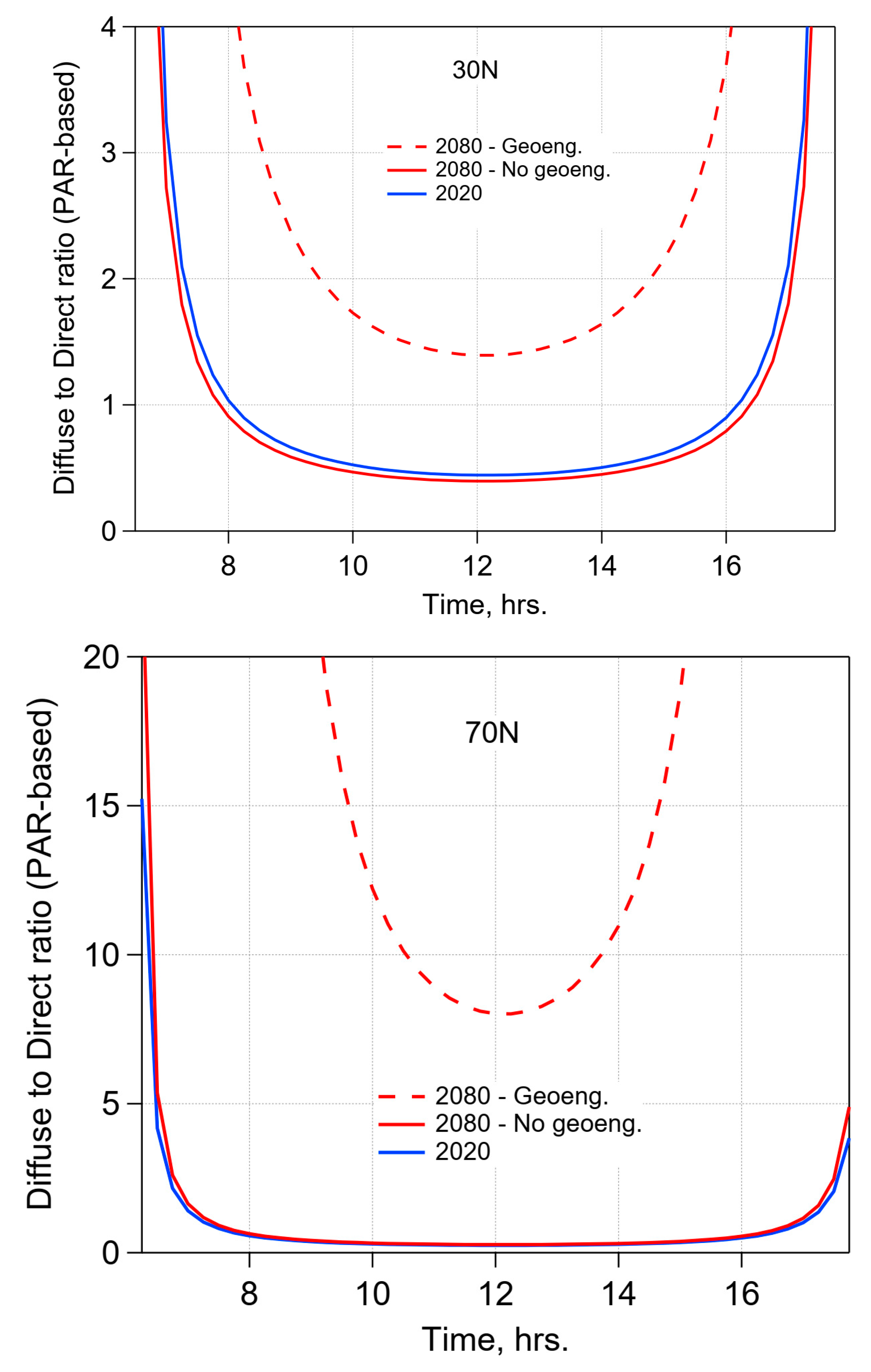
The diffuse-direct ratios for PAR radiation are shown in Figure 5 for the various scenarios. In 2020 and in the 2080 cases without geoengineering, noontime diffuse irradiance was less than half of the direct irradiance at 30 N, and less than a quarter at 70 N. By comparison, for idealized aerosol-free conditions (molecular absorption and Rayleigh scattering only), the PAR-based diffuse-direct ratio at high sun would be about 0.08, so these moderate ratios show the effect of background (without geoengineering) sulfate and other (mostly tropospheric) aerosols included in this model [24]. With geoengineering, the diffuse irradiance becomes dominant, as shown in Figure 5. At 30 N, the noontime diffuse component becomes nearly twice the direct component (i.e., a factor of 4 increase in the ratio compared to 2020). This was despite the fact that the noontime total PAR was only slightly lower (see Figure 4). At 70 N, the diffuse-direct ratio was never lower than about 7, which, combined with the 30% reduction in total PAR, implied notable modification to the color and brightness of the sky, as well as the photosynthetic rates. These results were qualitatively consistent with those obtained in earlier studies [19,20,21], with precise values depending on location, season, scenario, and, to some extent, model formulation.
3.2. Diurnal Cylces of Tropospheric Photo-Dissociation Rate Coefficients
Perturbations to UV actinic fluxes could have a significant effect on tropospheric photochemistry (e.g., evolution of oxidant gases and secondary aerosols). Figure 6 shows the effect on two important tropospheric photo-dissociation coefficients, jO1D and jNO2. Under the RCP8.5 without geoengineering scenario, jNO2 was expected to be largely unaffected (with similar sulfate loadings compared to 2020, see Table 2), while jO1D decreased, due to the recovery in stratospheric O3, by ca. 10% at 30 N and 20% at 70 N. With geoengineering, jO1D reductions were expected to double, to about 20% and 40% at 30 N and 70 N, respectively. On the other hand, the effects on jNO2 showed a stronger dependence on solar zenith angles (see the diurnal dependence in Figure 6), with little or no reduction at high sun. The high sun behavior resulted from the partial cancellation of two effects: (i) A reduction in total irradiance due to aerosol scattering; and (ii) an increase in diffuse irradiance, which contributed more effectively to the actinic flux than the direct beam (e.g., by 2cos(sza) in the isotropic limit) [42]. The relative timing of jNO2 to jO1D is of some importance to the chemical evolution of urban pollutants (e.g., the HO2–OH ratio, and its changes, would need to be considered in models of future air quality). While an analysis of the response of tropospheric chemistry to UV changes is beyond the scope here, we note that the sign of the expected change in tropospheric O3 depends on the amount of nitrogen oxides (NOx) present [43,44], and may be different on urban scales, rather than on regional or global scales [7,45,46].
3.3. Daily Average Values and Seasonal Trends
Table 3 gives the seasonal dependence of the radiation changes for the with geoengineering and without geoengineering scenarios, relative to current conditions (2020). The changes generally persisted throughout the year, but some patterns were notable: Relative reductions in transmission were generally greatest in December and at high latitudes (i.e., at small sun elevation angles), where they were most severe at visible wavelengths. Excluding December, the March reductions in jO1D, iDNA, and UVI were slightly more than those found for June or September (due to the seasonal dependence of the O3 column change, see Figure S1), whereas those for jNO2 and PAR remained unchanged (being dependent on the relatively constant sulfate column, see again Figure S1).
3.4. Impact of Sulfur Species
The direct impact of sulfate on the radiation field was evaluated by comparing TUV simulations, in which the scattering by sulfate (and absorption by SO2 gas) was either included or turned off. The results of such a calculation indicated that sulfate reduces the radiation by about 6% or less for the 2020 and 2080 scenarios, at both latitudes, without geoengineering. However, the geoengineering scenario led to reductions of 12% to 18% at 30 N, but ranged from 8% to 42% at 70 N. Finally, we note that substantial amounts of gaseous SO2 were present in the geoengineering scenario, ranging from about 0.3 Dobson units (DU) at 70 N, to about 0.9 DU at 30 N (see Table 1, and Figure S1). The UV absorption, by such amounts of SO2, reduced surface jO1D, iDNA, and UVI by about 1% at 30 N and about 0.2% at 70 N (i.e., substantially smaller than the effects of O3 absorption or sulfate scattering).
4. Discussion
A limitation of our study was that the UV and visible calculations were made assuming cloud-free conditions. Clouds were, of course, included in the CESM1(WACCM) model along with numerous other feedbacks, but not in the offline TUV calculations. The zonal averages used here cannot represent the high spatial and temporal variability of clouds, which stems mostly from local and regional meteorological processes, rather than the global changes in stratospheric sulfate and ozone of interest here. Thus, we focused on clear-sky values rather than (e.g., averages that included the long-term effects of local clouds). The clear-sky values permitted well-defined comparisons between observations and model results, whereas the variability associated with clouds could potentially mask the effects of stratospheric composition changes. We recognize, nevertheless, that cloud-induced changes in surface radiation are significant, and could also be subject to long-term changes.
If cloud cover is considered to remain constant over time (or between scenarios), the relative changes presented here (Table 3; Figure 4 and Figure 6) should still be reasonable estimates, because the sulfate aerosols would remain well above tropospheric clouds, notwithstanding some increase in multiple scattering between cloud and air. To test this, we repeated one calculation with a single horizontally infinite cloud, placed between 4 and 5 km above sea level (optical depth = 32) in all the scenarios. The results (see Table S1, Supplementary Materials) showed that for high sun, the fractional irradiance reduction due to aerosols was essentially the same whether clouds were present or not (comparing Table S1 and Table 3), and could, therefore, be considered independently. However, at low sun (70 N, winter), multiple scattering between clouds and aerosols led to some compensation, so that the fractional effect of aerosols was not as large as it would be under cloud-free skies.
Climate change and geoengineering will modify clouds differently, and these changes may be more important locally than changes in stratospheric sulfate or ozone. Future studies could take advantage of model-predicted cloud cover, and thus compute surface radiation for specific locations that accounts for local meteorology, and distinguishing, for example, for differences in cloud cover between ocean and land. Sensitivity studies could be used to separate the direct optical effects, due to stratospheric composition change, using, for example, clear sky values, from those due to climatological cloud cover and those resulting from climate-induced trends in cloud cover. We note; however, that the prediction of future cloudiness remains a major uncertainty in climate models [1].
We investigated here, one scenario that required a large amount of SO2 injection per year (about 40 TgSO2/year) to counteract up to 4 °C of surface warming. This amount would be required in 2080 if geoengineering were to be applied without stringent mitigation options set into place. Reduced injection amounts in earlier periods would be expected to show a different outcome, but have not been considered here. Our results for fairly large SO2 injections can probably be down-scaled for smaller injections, as changes in the sulfate optical depth were approximately correlated to SO2 injections. However, other changes, for example, in the O3 column, as the result of changes in water vapor, temperature, and circulation, with climate change and geoengineering, may play a significant role, and thus could invalidate simple downscaling that requires case-specific analyses.
Many other sources of uncertainty can be identified, from the choice of representative biological-action spectra to the optical properties of the aerosols. Empirical validation of our model was difficult due to the sparsity of relevant data. The spectral diffuse and direct ratio was measured by Zeng et al. [17] before and after the Mt. Pinatubo eruption (est. 18 TgSO2), and showed overall good agreement when vertical profile data (e.g., from ozone sondes) were available. However, if profile information is not available, large errors can occur.
5. Summary and Conclusions
Substantial changes in biologically active irradiances for DNA damage (iDNA), UV index (UVI), photosynthetically active radiation (PAR), and two key tropospheric photo-dissociation coefficients (jO1D and jNO2) were identified for a geoengineering experiment that would counteract surface warming between 2020 and 2080, while following the RCP8.5 scenario. Increases in column O3, due to the super-recovery in this scenario, played some role in reducing iDNA, UVI, and jO1D, whereas PAR and jNO2 were mostly unaffected by O3 changes. However, additional reductions in iDNA, UVI, and jO1D, and larger reductions in both PAR and jNO2, in high latitudes in particular, occurred for the geoengineering scenario.
Different results can be further expected, depending on scenarios, different models, and even aerosol type [47,48,49,50]. For example, while our results using the CESM1(WACCM) simulations indicated an increase in the O3 column from geoengineering between 2020 and 2080 due to super-recovery at 30 N and 70 N, Eastham et al. [22] considered scenarios with reduced O3 column, and estimated the associated UV-driven increased mortality from skin cancer to be more than offset by gains in regional air quality. However, there are wide gaps in the understanding of how air pollutants, such as ambient ozone and PM, respond to changes in UV-induced photochemistry [45,46] and other environmental conditions, and, in some cases, even the direction of change is unknown.
Thus, here we focused in more detail on the physical changes of the radiation field impingent on the surface, and its direct impact on photochemical drivers, such as jNO2 and jO1D, and biologically active irradiances iDNA, UVI, and PAR. Each of these responded somewhat differently to the scenarios, due to different directional and wavelength sensitivities. The perturbation of the radiation field by sulfate depended on wavelength and sza, led to higher diffuse-direct ratios, and induced somewhat different daily and seasonal light cycles. Twilight would be extended, particularly at high latitudes. Reductions at UV wavelengths would not be as strong as at visible wavelengths, due to single and multiple scattering phenomena. Most importantly, these changes would occur on global scales and persist for years, and, though fully recognizing the uncertainties in our calculations, we are concerned that deeper studies are needed on how such marked changes in the UV and visible sky would affect humans and ecosystems.
Supplementary Materials
The following are available online at https://www.mdpi.com/2073-4433/9/11/432/s1, Figure S1: Seasonally resolved differences in column-integrated amounts of O3, sulfate, and SO2 for current conditions (black squares), and in 2080 with (blue circles) or without (red triangles) geoengineering (RCP8.5), for 30 N (solid) and 70 N (dashed), Table S1: Effect(a) of cloud cover on future changes in surface photochemical (jO1D and jNO2) and photobiological (iDNA, UVI, and PAR) radiation, as ratios of values in 2080 to 2020, with and without NO geoengineering by stratospheric SO2 injections.
Author Contributions
Conceptualization: S.M. and S.T.; CESM1(WACCM) design: S.T., D.G.M., B.K., and J.R.; CESM1(WACCM) simulations: S.T.; TUV simulations: S.M.; original draft preparation: S.M. and S.T.; writing, reviewing, and editing: S.M., S.T., B.K., D.G.M., and J.H.R.
Funding
This research received no external funding.
Acknowledgments
The CESM project is supported by the National Science Foundation and the Office of Science (BER) of the U.S. Department of Energy. The National Center for Atmospheric Research is sponsored by the National Science Foundation. The Pacific Northwest National Laboratory is operated for the U.S. Department of Energy by Battelle Memorial Institute under contract DE-AC05-76RL01830.
Conflicts of Interest
The authors declare no conflicts of interest.
References
- IPCC. Climate Change 2013: The Physical Science Basis; Contribution of Working Group I to the Fifth Assessment Report of the Intergovernmental Panel on Climate Change; Stocker, T.F., Qin, D., Plattner, G.-K., Tignor, M., Allen, S.K., Boschung, J., Nauels, A., Xia, Y., Bex, V., Midgley, P.M., Eds.; Cambridge University Press: Cambridge, UK; New York, NY, USA, 2013; 1535p. [Google Scholar]
- Budyko, M.I. Climate and Life; Academic Press: New York, NY, USA, 1974; pp. 1–508. [Google Scholar]
- Crutzen, P.J. Albedo enhancement by stratospheric sulfur injections: A contribution to resolve a policy dilemma? Clim. Chang. 2006, 77, 211–220. [Google Scholar] [CrossRef]
- Niemeier, U.; Tilmes, S. Sulfur injections for a cooler planet. Science 2017, 357, 246–248. [Google Scholar] [CrossRef] [PubMed]
- Tilmes, S.; Garcia, R.R.; Kinnison, D.E.; Gettelman, A.; Rasch, P.J. Impact of geoengineered aerosols on the troposphere and stratosphere. J. Geophys. Res. 2009, 114, D12305. [Google Scholar] [CrossRef]
- Pitari, G.; Aquila, V.; Kravitz, B.; Robock, A.; Watanabe, S.; Cionni, I.; Luca, N.D.; Genova, G.D.; Mancini, E.; Tilmes, S. Stratospheric ozone response to sulfate geoengineering: Results from the Geoengineering Model Intercomparison Project (GeoMIP). J. Geophys. Res. 2014, 119, 2629–2653. [Google Scholar] [CrossRef] [Green Version]
- Xia, L.; Nowack, P.J.; Tilmes, S.; Robock, A. Impacts of stratospheric sulfate geoengineering on tropospheric ozone. Atmos. Chem. Phys. 2017, 17, 11913–11928. [Google Scholar] [CrossRef] [Green Version]
- Kravitz, B.; MacMartin, D.G.; Mills, M.J.; Richter, J.H.; Tilmes, S.; Lamarque, J.-F.; Tribbia, J.J.; Vitt, F. First simulations of designing stratospheric sulfate aerosol geoengineering to meet multiple simultaneous climate objectives. J. Geophys. Res. 2017, 122, 12616–12634. [Google Scholar] [CrossRef]
- Richter, J.H.; Tilmes, S.; Mills, M.J.; Tribbia, J.J.; Kravitz, B.; MacMartin, D.G.; Vitt, F.; Lamarque, J.-F. Stratospheric dynamical response to SO2 injections. J. Geophys. Res. 2017, 122, 12557–12573. [Google Scholar] [CrossRef]
- Tilmes, S.; Richter, J.H.; Mills, M.J.; Kravitz, B.; MacMartin, D.G.; Garcia, R.R.; Kinnison, D.E.; Lamarque, J.-F.; Tribbia, J.; Vitt, F. Effects of different stratospheric SO2 injection altitudes on stratospheric chemistry and dynamics. J. Geophys. Res. 2018, 123, 4654–4673. [Google Scholar] [CrossRef]
- Ji, D.; Fang, S.; Curry, C.L.; Kashimura, H.; Watanabe, S.; Cole, J.N.S.; Lenton, A.; Muri, H.; Kravitz, B.; Moore, J.C. Extreme temperature and precipitation response to solar dimming and stratospheric aerosol geoengineering. Atmos. Chem. Phys. 2018, 18, 10133–10156. [Google Scholar] [CrossRef]
- Michelangeli, D.V.; Allen, M.; Yung, Y.L. El Chichon volcanic aerosols: Impact of radiative, thermal, and chemical perturbations. J. Geophys. Res. 1989, 94, 18429–18442. [Google Scholar] [CrossRef] [PubMed]
- Michelangeli, D.V.; Allen, M.; Yung, Y.L.; Shia, R.-L.; Crisp, D.; Eluszkiewicz, J. Enhancement of atmospheric radiation by an aerosol layer. J. Geophys. Res. 1992, 97, 865–874. [Google Scholar] [CrossRef] [PubMed] [Green Version]
- Davies, R. Increased transmission of ultraviolet radiation to the surface due to stratospheric scattering. J. Geophys. Res. 1993, 98, 7251–7253. [Google Scholar] [CrossRef]
- Tsitas, S.R.; Yung, Y.L. The effect of volcanic aerosols on ultraviolet radiation in Antarctica. Geophys. Res. Lett. 1996, 23, 157–160. [Google Scholar] [CrossRef] [Green Version]
- Vogelmann, A.M.; Ackerman, T.P.; Turco, R.P. Enhancement in biologically effective ultraviolet radiation following volcanic eruptions. Nature 1992, 359, 47–49. [Google Scholar] [CrossRef] [PubMed]
- Zeng, J.; McKenzie, R.; Stamnes, K.; Wineland, M.; Rosen, J. Measured UV spectra compared with discrete ordinate method simulations. J. Geophys. Res. 1994, 99, 23019–23030. [Google Scholar] [CrossRef]
- Gu, L.; Baldocchi, D.D.; Wofsy, S.C.; Munger, J.W.; Michalsky, J.J.; Urbanski, S.P.; Boden, T.A. Response of a deciduous forest to the Mount Pinatubo eruption: Enhanced photosynthesis. Science 2003, 299, 2035–2038. [Google Scholar] [CrossRef] [PubMed]
- Mercado, L.M.; Bellouin, N.; Sitch, S.; Boucher, O.; Huntingfort, C.; Wild, M.; Cox, P.M. Impact of changes in diffuse radiation on the global land carbon sink. Nature 2009, 458, 1014–1018. [Google Scholar] [CrossRef] [PubMed] [Green Version]
- Kravitz, B.; MacMartin, D.G.; Caldeira, K. Geoengineering: Whiter skies? Geophys. Res. Lett. 2012, 39, L121801. [Google Scholar] [CrossRef]
- Xia, L.; Robock, A.; Tilmes, S.; Neely, R.R., III. Stratospheric sulfate geoengineering could enhance terrestrial photosynthesis rate. Atmos. Chem. Phys. 2016, 16, 1479–1489. [Google Scholar] [CrossRef]
- Eastham, S.D.; Weisenstein, D.K.; Keith, D.W.; Barrett, S.R.H. Quantifying the impact of sulfate geoengineering on mortality from air quality and UV-B exposure. Atmos. Environ. 2018, 187, 424–434. [Google Scholar] [CrossRef]
- Hurrell, J.W.; Holland, M.M.; Gent, P.R.; Ghan, S.; Kay, J.E.; Kushner, P.J.; Lamarque, J.-F.; Large, W.G.; Lawrence, D.; Lindsay, K.; et al. The Community Earth System Model: A framework for collaborative research. Bull. Am. Meteor. Soc. 2013, 94, 1339–1360. [Google Scholar] [CrossRef]
- Mills, M.J.; Richter, J.H.; Tilmes, S.; Kravitz, B.; MacMartin, D.G.; Glanville, A.A.; Tribbia, J.J.; Lamarque, J.-F.; Vitt, F.; Schmidt, A.; et al. Radiative and chemical response to interactive stratospheric sulfate aerosols in fully coupled CESM1(WACCM). J. Geophys. Res. 2017, 122, 13061–13078. [Google Scholar] [CrossRef]
- Guenther, A.B.; Jiang, X.; Heald, C.L.; Sakulyanontvittaya, T.; Duhl, T.; Emmons, L.K.; Wang, X. The Model of Emissions of Gases and Aerosols from Nature version 2.1 (MEGAN2.1): An extended and updated framework for modeling biogenic emissions. Geosci. Model Dev. 2012, 5, 1471–1492. [Google Scholar] [CrossRef] [Green Version]
- Tilmes, S.; Richter, J.H.; Kravitz, B.; MacMartin, D.G.; Mills, M.J.; Simpson, I.R.; Glanville, A.S.; Fasullo, J.T.; Phillips, A.S.; Lamarque, J.; et al. CESM1(WACCM) Stratospheric Aerosol Geoengineering Large Ensemble (GLENS) Project. Bull. Amer. Meteor. Soc. 2018, in press. [Google Scholar] [CrossRef]
- MacMartin, D.G.; Kravitz, B.; Tilmes, S.; Richter, J.H.; Mills, M.J.; Lamarque, J.-F.; Tribbia, J.J.; Vitt, F. The climate response to stratospheric aerosol geoengineering can be tailored using multiple injection locations. J. Geophys. Res. 2017, 122, 12574–12590. [Google Scholar] [CrossRef]
- Koepke, P.; Bais, A.; Balis, D.; Buchwitz, M.; De Backer, H.; De Cabos, X.; Eckert, P.; Eriksen, P.; Gillotay, D.; Heikkila, A.; et al. Comparison of models used for UV index calculations. Photochem. Photobiol. 1998, 67, 657–662. [Google Scholar] [CrossRef] [PubMed]
- Bais, A.; Madronich, S.; Crawford, J.; Hall, S.R.; Mayer, B.; VanWeele, M.; Lenoble, J.; Calvert, J.G.; Cantrell, C.A.; Shetter, R.E.; et al. International photolysis frequency measurement and model intercomparison: Spectral actinic solar flux measurements and modeling. J. Geophys. Res. 2003, 108, 8543. [Google Scholar] [CrossRef]
- Palancar, G.G.; Lefer, B.L.; Hall, S.R.; Shaw, W.J.; Corr, C.A.; Herndon, S.C.; Slusser, J.R.; Madronich, S. Effects of aerosol and NO2 concentration on ultraviolet actinic flux near Mexico City during MILAGRO: Measurements and model calculations. Atmos. Chem. Phys. 2013, 13, 1011–1022. [Google Scholar] [CrossRef] [Green Version]
- Brogniez, C.; Lenoble, J.; Herman, M.; Lecomte, P.; Verwaerde, C. Analysis of two balloon experiments in coincidence with SAGE II in case of large stratospheric aerosol amount: Post-Pinatubo period. J. Geophys. Res. 1996, 101, 1541–1552. [Google Scholar] [CrossRef]
- World Health Organization (WHO). Global Solar UV Index; WHO: Geneva, Switzerland, 2002; ISBN 9241590076. [Google Scholar]
- Webb, A.R.; Slaper, J.; Koepke, P.; Schmalwieser, A.W. Know your standard: Clarifying the CIE erythema action spectrum. Photochem. Photobiol. 2011, 87, 483–486. [Google Scholar] [CrossRef] [PubMed]
- Setlow, R.B. The wavelengths in sunlight effective in producing skin cancer: A theoretical analysis. Proc. Natl. Acad. Sci. USA 1974, 71, 3363–3366. [Google Scholar] [CrossRef] [PubMed]
- Sutherland, J.C.; Griffin, K.P. Absorption spectrum of DNA for wavelengths greater than 300 nm. Radiat. Res. 1981, 86, 399–409. [Google Scholar] [CrossRef] [PubMed]
- McKenzie, R.L.; Aucamp, P.J.; Bais, A.F.; Björn, L.O.; Ilyas, M.; Madronich, S. Ozone depletion and climate change: Impacts on UV radiation. Photochem. Photobiol. Sci. 2011, 10, 182–198. [Google Scholar] [CrossRef] [PubMed]
- Burkholder, J.B.; Sander, S.P.; Abbatt, J.; Barker, J.R.; Huie, R.E.; Kolb, C.E.; Kurylo, M.J.; Orkin, V.L.; Wilmouth, D.M.; Wine, P.H. Chemical Kinetics and Photochemical Data for Use in Atmospheric Studies; Evaluation No. 18, JPL Publication No. 15-10; Jet Propulsion Laboratory: Pasadena, CA, USA, 2015. [Google Scholar]
- Madronich, S.; Granier, C. Impact of recent total ozone changes on tropospheric ozone photodissociation, hydroxyl radicals, and methane trends. Geophys. Res. Lett. 1992, 19, 465–467. [Google Scholar] [CrossRef]
- USSA. US Standard Atmosphere; National Oceanic and Atmospheric Administration (NOAA), National Aeronautics and Space Administration (NASA), United States Air Force (USAF), US Government Printing Office: Washington, DC, USA, 1976; 241p.
- Wängberg, S.A.; Selmer, J.-S.; Egelund, N.G.A.; Gustavson, K. UV-B Effects on Nordic Marine Exocystems: A Literature Review; TemaNord 1996:515; Nordic Council of Ministers: Copenhagen, Denmark, 1996; ISBN 929120823X. [Google Scholar]
- Rozema, J.; Boelen, P.; Blokker, P. Depletion of stratospheric ozone over the Antarctic and Arctic: Responses of plants of polar terrestrial ecosystems to enhanced UV-B, an overview. Environ. Pollut. 2005, 137, 428–442. [Google Scholar] [CrossRef] [PubMed]
- Madronich, S. Photodissociation in the atmosphere 1. Actinic flux and the effects of ground reflections and clouds. J. Geophys. Res. 1987, 92, 9740–9752. [Google Scholar] [CrossRef]
- Liu, S.C.; Trainer, M. Responses of the tropospheric ozone and odd hydrogen radicals to column ozone change. J. Atmos. Chem. 1988, 6, 221–233. [Google Scholar] [CrossRef]
- Thompson, A.M.; Stewart, R.W.; Owens, M.A.; Herwehe, J.A. Sensitivity of tropospheric oxidants to global chemical and climate change. Atmos. Environ. 1989, 23, 519–532. [Google Scholar] [CrossRef]
- Zhang, H.; Wu, S.; Huang, Y.; Wang, Y. Effects of stratospheric ozone recovery on photochemistry and ozone air quality in the troposphere. Atmos. Chem. Phys. 2014, 14, 4079–4089. [Google Scholar] [CrossRef] [Green Version]
- Hodzic, A.; Madronich, S. Response of surface ozone over the continentalUnited States to UV radiation declines from the expectd recovery of stratospheric ozone. Nat. Clim. Atmos. Sci. 2018. [Google Scholar] [CrossRef]
- Tang, M.J.; Telford, P.J.; Pope, F.D.; Rkiouak, L.; Abraham, N.L.; Archibald, A.T.; Braesicke, P.; Pyle, J.A.; McGregor, J.; Watson, I.M.; et al. Heterogeneous reaction of N2O5 with airborne TiO2 particles and its implication for stratospheric particle injection. Atmos. Chem. Phys. 2014, 14, 6035–6048. [Google Scholar] [CrossRef]
- Tang, M.; Keeble, J.; Telford, P.J.; Pope, F.D.; Braesicke, P.; Griffiths, P.T.; Abraham, N.L.; McGregor, J.; Watson, I.M.; Cox, R.A.; et al. Heterogeneous reaction of ClONO2 with TiO2 and SiO2 aerosol particles: Implications for stratospheric particle injection for climate engineering. Atmos. Chem. Phys. 2016, 16, 15397–15412. [Google Scholar] [CrossRef]
- Weisenstein, D.K.; Keith, D.W.; Dykema, J.A. Solar geoengineering using solid aerosol in the stratosphere. Atmos. Chem. Phys. 2015, 315, 11835–11859. [Google Scholar] [CrossRef]
- Keith, D.W.; Weisenstein, D.K.; Dykema, J.A.; Keutsch, F.N. Stratospheric solar geoengineering without ozone loss. Proc. Nat. Acad. Sci. USA 2016, 113, 14910–14914. [Google Scholar] [CrossRef] [PubMed]
Figure 1.
The zonal averaged stratospheric sulfate aerosol distribution for the geoengineering experiment in March 2080. The black curve shows approximate tropopause location.
Figure 1.
The zonal averaged stratospheric sulfate aerosol distribution for the geoengineering experiment in March 2080. The black curve shows approximate tropopause location.

Figure 2.
The vertical profiles of O3 concentration (left) and sulfate aerosol extinction at 550 nm (right), zonally averaged at 30 N (top) and 70 N (bottom). The legend indicates the years depicted, all of which present March average data, for current day (2020) and future (2080) scenarios without and with geoengineering.

Figure 3.
Changes in ground-level DNA-damaging irradiance (x-axis), when adding a hypothetical, 1 km thick, single aerosol layer (optical depth = 0.2), at different altitudes (y-axis) in an otherwise aerosol-free atmosphere.
Figure 3.
Changes in ground-level DNA-damaging irradiance (x-axis), when adding a hypothetical, 1 km thick, single aerosol layer (optical depth = 0.2), at different altitudes (y-axis) in an otherwise aerosol-free atmosphere.

Figure 4.
Changes in biologically active radiation at the Earth’s surface, in March 2080 relative to March 2020, for DNA-weighted irradiance iDNA (blue), UV index (UVI) (red), and photosynthetically active radiation PAR (green), without geoengineering (solid curves) and with geoengineering (dashed curves). The black curve and right axis refer to solar zenith angle.

Figure 5.
Ratio of diffuse sky radiation to direct solar beam at the surface, for the current atmosphere (March 2020, blue curve) and scenarios for March 2080 without geoengineering (red, solid) and with geoengineering by sulfur injection (red, dash). Based on photosynthetically available radiation (PAR) between 400 and 700 nm.

Figure 6.
Changes for key tropospheric photolysis coefficients, for the reactions NO2 + hν → NO + O (jNO2, red) and O3 + hν → O2 + O(1D) (jO1D, blue), for March 2080 relative to current day (March 2020), without geoengineering (solid curves) and with geoengineering (dashed curve). The black curve and right axis refer to solar zenith angle.


Table 1.
The simulations used in this study performed with the Community Earth System Model, version 1 (CESM1), using the Whole Atmosphere Community Climate Model (WACCM) as its atmospheric component.
Table 1.
The simulations used in this study performed with the Community Earth System Model, version 1 (CESM1), using the Whole Atmosphere Community Climate Model (WACCM) as its atmospheric component.
| Simulation | Simulation Time | Ensemble Members | Year Used a |
|---|---|---|---|
| RCP8.5 | 2010–2030 | 17 | 2020 |
| RCP8.5, no geoengineering | 2010–2097 | 3 | 2080 |
| RCP8.5, with geoengineering | 2020–2099 | 20 | 2080 |
a Year(s) for which the monthly data were analyzed in the present study. RCP8.5: Representative Concentration Pathway 8.5.
Table 2.
The column optical properties for current and future conditions (March) from the CESM1(WACCM) simulations.
Table 2.
The column optical properties for current and future conditions (March) from the CESM1(WACCM) simulations.
| 30 N | 2020 | 2080 | |
|---|---|---|---|
| Current | Without Geoeng. | With Geoeng. | |
| O3, DU a | 280 | 296 | 307 |
| SO2, DU | 0.17 | 0.07 | 0.88 |
| Ext. 350 b | 0.31 | 0.25 | 0.81 |
| Ext. 550 | 0.28 | 0.24 | 0.80 |
| Ext. 1020 | 0.24 | 0.23 | 0.64 |
| 70 N | |||
| O3, DU | 428 | 487 | 491 |
| SO2, DU | 0.03 | 0.01 | 0.25 |
| Ext. 350 | 0.02 | 0.03 | 0.90 |
| Ext. 550 | 0.02 | 0.03 | 0.89 |
| Ext. 1020 | 0.01 | 0.02 | 0.64 |
a Dobson unit, 1 DU = 2.687 × 10¹⁶ molecules cm−2. b Aerosol optical depth at indicated wavelength (nm).
Table 3.
Future changes in surface photochemical (jO1D and jNO2) and photobiological (iDNA, UVI, and PAR) radiation, as ratios of values in 2080 to 2020, with and without geoengineering by stratospheric SO2 injections. Based on daily average values for the months indicated.
Table 3.
Future changes in surface photochemical (jO1D and jNO2) and photobiological (iDNA, UVI, and PAR) radiation, as ratios of values in 2080 to 2020, with and without geoengineering by stratospheric SO2 injections. Based on daily average values for the months indicated.
| ilat | Without Geoengineering | With Geoengineering | ||||||||
|---|---|---|---|---|---|---|---|---|---|---|
| 30 N | jO1D | jNO2 | iDNA | UVI | PAR | jO1D | jNO2 | iDNA | UVI | PAR |
| March | 0.92 | 1.01 | 0.89 | 0.94 | 1.01 | 0.76 | 0.91 | 0.71 | 0.80 | 0.90 |
| June | 0.94 | 1.01 | 0.92 | 0.96 | 1.01 | 0.79 | 0.94 | 0.73 | 0.81 | 0.92 |
| September | 0.96 | 1.01 | 0.94 | 0.97 | 1.01 | 0.80 | 0.91 | 0.77 | 0.83 | 0.90 |
| December | 0.94 | 1.01 | 0.92 | 0.96 | 1.00 | 0.73 | 0.82 | 0.73 | 0.80 | 0.84 |
| 70 N | ||||||||||
| March | 0.82 | 0.99 | 0.81 | 0.90 | 0.98 | 0.65 | 0.59 | 0.73 | 0.77 | 0.66 |
| June | 0.83 | 1.00 | 0.79 | 0.89 | 0.99 | 0.71 | 0.77 | 0.73 | 0.79 | 0.79 |
| September | 0.85 | 0.99 | 0.83 | 0.91 | 0.98 | 0.77 | 0.65 | 0.86 | 0.85 | 0.72 |
| December | 0.77 | 0.94 | 0.77 | 0.85 | 0.94 | 0.64 | 0.44 | 0.61 | 0.63 | 0.22 |
© 2018 by the authors. Licensee MDPI, Basel, Switzerland. This article is an open access article distributed under the terms and conditions of the Creative Commons Attribution (CC BY) license (http://creativecommons.org/licenses/by/4.0/).
Share and Cite
MDPI and ACS Style
Madronich, S.; Tilmes, S.; Kravitz, B.; MacMartin, D.G.; Richter, J.H. Response of Surface Ultraviolet and Visible Radiation to Stratospheric SO2 Injections. Atmosphere 2018, 9, 432. https://doi.org/10.3390/atmos9110432
AMA Style
Madronich S, Tilmes S, Kravitz B, MacMartin DG, Richter JH. Response of Surface Ultraviolet and Visible Radiation to Stratospheric SO2 Injections. Atmosphere. 2018; 9(11):432. https://doi.org/10.3390/atmos9110432
Chicago/Turabian StyleMadronich, Sasha, Simone Tilmes, Ben Kravitz, Douglas G. MacMartin, and Jadwiga H. Richter. 2018. "Response of Surface Ultraviolet and Visible Radiation to Stratospheric SO2 Injections" Atmosphere 9, no. 11: 432. https://doi.org/10.3390/atmos9110432
Note that from the first issue of 2016, this journal uses article numbers instead of page numbers. See further details here.