 Andrea Kaim
 Michael Strauch
 Martin Volk
- 1Professorship of Ecological Services, University of Bayreuth, Bayreuth, Germany
- 2Department Landscape Ecology, Helmholtz Centre for Environmental Research-UFZ, Leipzig, Germany
One way to solve multi-objective spatial land use allocation problems is to calculate a set of Pareto-optimal solutions and include stakeholder preferences after the optimization process. There are various land use allocation studies that identify the Pareto frontier (i.e., trade-off curve); to our knowledge, however, for the majority of them, the debate on which solutions are preferred by stakeholders or are preferred by stakeholders remains open. One reason could be that Pareto-optimal solutions, due to their multi-dimensionality, are difficult to communicate. To fill this gap, we give an example using the results of a multi-objective agricultural land use allocation problem that maximizes four biophysical objectives: agricultural production, water quality, water quantity, and biodiversity in the Lossa River Basin in Central Germany. We conducted expert interviews with 11 local stakeholders from different backgrounds, e.g., water experts, nature conservationists, farmers, etc. In addition to providing information about the case study area, we visualized the trade-offs between the different objectives using parallel coordinates plots that allowed the stakeholders to browse through the optimal solutions. Based on this information, the stakeholders set weights for each of the objectives by applying the Analytic Hierarchy Process (AHP). With these weights, we selected the preferred solutions from the Pareto-optimal set. The results show that, overall, stakeholders clearly ranked water quality first, followed by biodiversity, water quantity, and agricultural production. The corresponding land use maps show a huge difference in land management (e.g., less application of fertilizer, more linear elements, and conservation tillage) for the preferred solutions compared to the current status. The method presented in this study can help decision makers finding land use and land management strategies based on both biophysical modeling results and stakeholder expertise, and it shows how multi-objective optimization results can be communicated and used for an information-based decision-making process.
1. Introduction
Multi-objective optimization is frequently used to solve land use allocation problems. Pareto-optimization in particular is used to analyze trade-offs and synergies between different objectives (Kaim et al., 2018). The benefit of this method is that it provides a whole set of “optimal” solutions that span the entire range of the objective function values and thus offers a wide choice of options for the decision maker. In contrast to scenario building or optimization methods that include stakeholder preferences a priori (i.e., before the optimization), Pareto-optimization allows the stakeholders to form their preferences by informing them about synergies and trade-offs between the different objectives. However, this approach can also become challenging when it comes to communicating the optimization results to stakeholders since these problems can involve many objectives that easily lead to a couple of thousand Pareto-optimal solutions. In fact, almost all land use allocation studies that identify and analyze the Pareto-frontier end at this stage of the process.
An important aspect of communicating the optimization results to stakeholders is the visualization of Pareto-optimal solutions. There are a variety of methods available from multi-dimensional plots (e.g., Kollat and Reed, 2007; Lautenbach et al., 2013) and parallel coordinates plots (Inselberg and Dimsdale, 1990) over spider charts (Miettinen, 2014) to hyper-radial visualization (Chiu et al., 2009) to name only a few of them. For an overview of different visualization methods we refer to Lotov and Miettinen (2008). But despite all these options, not all visualization methods are equally suitable for land use allocation problems. For instance, multi-dimensional plots quickly become very difficult to read for stakeholders once they illustrate solutions for more than 2–3 objectives. The same holds for most other visualization methods: the more objectives an optimization problem has the more difficult is the visualization.
Generally, there are two methods of selecting solutions from the Pareto-frontier: pruning and ranking. Pruning involves techniques that reduce the set of optimal solutions, such as self-organizing maps (e.g., Li et al., 2009), subtractive clustering (Zio and Bazzo, 2011), or box indices (Miettinen et al., 2009). In the end, these solutions can either be ranked, or stakeholders can select directly from the reduced set. Ranking the set of Pareto-optimal solutions can be done by applying methods like the weighted stress function (Ferreira et al., 2008) or methods from multi-criteria decision making, such as outranking methods (Bouyssou, 2001) or pairwise comparisons. A prominent method for the latter is Saaty's Analytic Hierarchy Process (AHP) (Saaty, 1988) of which we will provide a detailed explanation later. A comparison of different pruning and ranking methods with examples from the field of traffic and transportation research that are also applicable to land use allocation problems can be found in Wismans et al. (2014).
An example of a study from agricultural land use allocation that uses pruning and ranking can be found in Chikumbo et al. (2014). The authors identified the Pareto-optimal set of a 14-objective land use management problem. They used hyper-radial visualization to select four solutions out of this set and then applied the AHP identifying the preferred solution by the stakeholders. There are only few other studies that aim at selecting a preferred solution after identifying the Pareto-optimal set (i.e., a posteriori preference articulation). Examples can be found in forest management (e.g., Borges et al., 2017; Marto et al., 2018) or in other research fields, such as transportation optimization (Ojha et al., 2010), supply-chain management (Ayadi et al., 2017), or electric distribution network planning (Celli et al., 2018). To our knowledge, the study by Chikumbo et al. (2014) is the only one in agricultural land use allocation that might partly be caused by a lack of communication between different research areas (Memmah et al., 2015).
To fill this gap, we present a framework for the selection of one or multiple preferred solution(s) from the Pareto-frontier of an agricultural land use allocation problem using stakeholder preferences. In the framework, we apply parallel coordinates plots for the visualization of the Pareto-optimal solutions and the AHP to weight the objectives and identify the preferred solution(s).
Our approach differs from the one presented by Chikumbo et al. (2014). First, our optimization process provides solutions over the entire range of objective function values, while Chikumbo et al. (2014) searched for Pareto-optimal solutions close to reference points in order to cope with the extremely large solution space that comes with a many-objective optimization problem. Second, in Chikumbo et al. (2014), the AHP was applied to select the preferred solution out of four scenario solutions that were previously identified by pruning. In our case, the AHP weights were used to select the preferred solutions(s) from the entire Pareto-optimal set (i.e., we followed a pure ranking approach).
We apply the framework to the results of a multi-objective spatial land use allocation problem that is based at the conflict between agricultural production, biodiversity conservation, and enhancing water quality and quantity. Although there has been considerable success in recent decades, water pollution by nutrients originating from agricultural practices remains a key problem in Europe (European Environment Agency, 2018). Furthermore, agricultural production is considered as one of the main drivers of biodiversity loss, which is reflected in an ongoing decline in farmland birds (a typical measure for farmland biodiversity) (Busch et al., 2020). The optimization problem considered in this study therefore aims to maximize biodiversity, water quality and quantity, and agricultural production in a river basin in Central Germany. The optimization results originate from research conducted within the project “Towards Multifunctional Agricultural Landscapes in Europe—TALE” (TALE, 2020) and merely serve as input data for our framework. For their detailed discussion we refer to Strauch et al. (2018).
2. Materials and Methods
The framework for the selection of preferred solution(s) from the Pareto-optimal set is summarized in Figure 1. It starts with the information of stakeholders about the case study area and optimization results, followed by the identification of preferences that are later used for the selection process. Each step of the framework requires certain methods or input data. We will therefore first give an overview of the case study area and the optimization results that served as input data for our study. We will then briefly explain the visualization (parallel coordinates plots) and the weighting (Analytic Hierarchy Process) methods that are fundamental to the stakeholder interviews that will be presented after these. Finally, we will explain how the preference information has been used for the selection of a preferred solution.
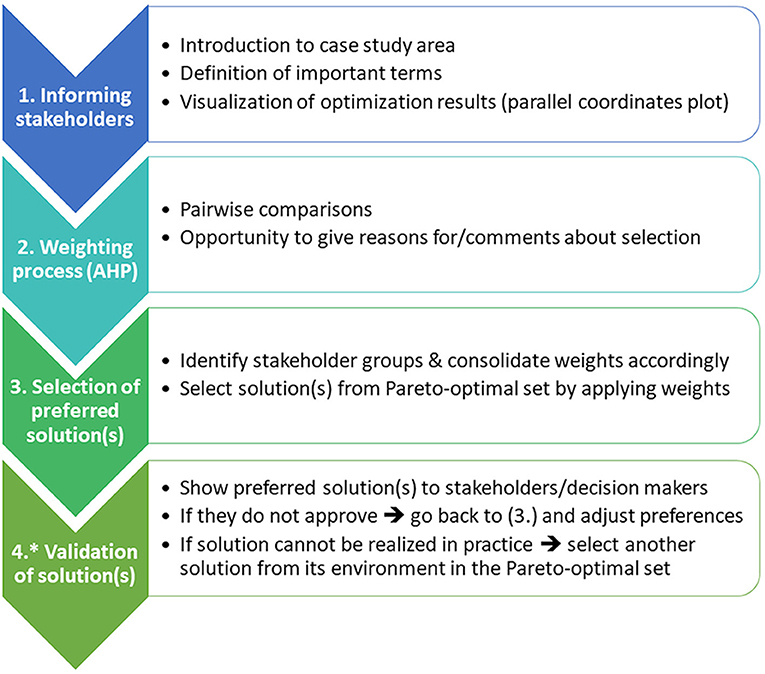
Figure 1. Framework for the identification of preferred solutions from the set of Pareto-optimal solutions. Steps 1–3 were implemented in this research, 4* could be added in future work.
2.1. Case Study Area and Land Management Scenarios
The 14,076 ha large Lossa River Basin is located in Central Germany and is characterized by a large proportion of agricultural land (see Figure 2). It is a subbasin of the Middle Mulde River Basin, for which the TALE project (TALE, 2020) developed four different land management scenarios within a stakeholder workshop: status quo (SQ)—describing the current situation, business as usual (BAU)—assuming a continuation of current trends until the year 2030, land sharing (LSH)—basically describing an extensification, and land sparing (LSP)—describing an intensification in agricultural production (note that LSP also involved restoring or creating some non-farmland habitat (e.g., “set aside” areas and forests) on arable land; however, this was predominantly on spots outside the Lossa River Basin). The general stakeholder process is explained in Karner et al. (2019) and Hagemann et al. (2020), and in the TALE Learning Environment (TALE, 2020).
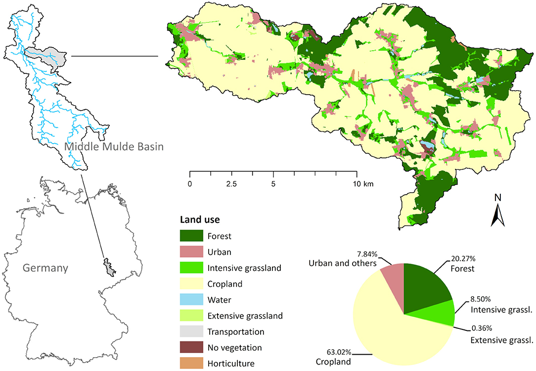
Figure 2. Location, land use map, and land use distribution of the Lossa River Basin.
For the total area of the Middle Mulde River Basin, farmers, conservationists, and employees of state agencies who relate to the area were invited to discuss how land management would change within the different scenarios. The results, specifically analyzed for the Lossa Basin, are summarized in Table 1. Major differences between the scenarios relate to the share of single crops (e.g., less/more rapeseed in LSH/LSP) and types of grassland (e.g., more extensive in LSH), the amount of applied fertilizer (less/more nitrate and phosphorus in LSH/LSP), and the type of tillage practices (e.g., only conservation tillage in LSH). Furthermore, differences in the share of linear elements, for example, hedgerows, lines of trees or field margins (e.g., larger/smaller in LSH/LSP), and urban area (e.g., largest increase in BAU and no increase in LSP) were considered. In the Lossa Basin, organic farming increases only slightly in scenarios BAU and LSH, although the increase of organic farming in LSH was substantial (up to 20%) for the whole Middle Mulde Basin. Similar to the “set aside” areas dedicated for afforestation in LSP, cropland with an increasing proportion of organic farming in LSH was predominantly located outside the Lossa Basin. LSP assumes no organic farming at all.
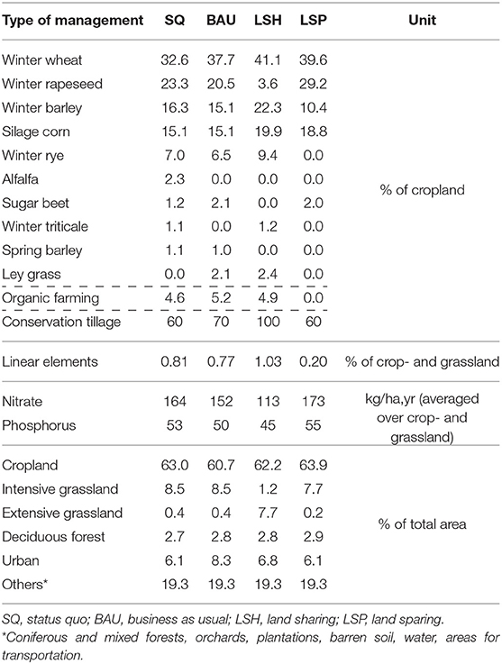
Table 1. Land management of the Lossa River Basin under different scenarios.
2.2. Optimization Results (Input Data)
The scenarios were used to formulate a multi-objective land use allocation problem that aimed to maximize water quality (i.e., minimal nitrate load leaving the Lossa River Basin in [kgN/a]), water quantity during low-flow periods at the basin outlet (mean annual minimum flow in [l/s]), agricultural production (contribution margins in [€/a]), and biodiversity (bird habitat index) in the study area. For this purpose, the Lossa River Basin was divided into 243 hydrologic response units (HRUs). HRUs are patches of similar characteristics like land uses, soil types, and slope. They form the smallest unit of the Soil and Water Assessment Tool (SWAT) (Arnold and Fohrer, 2005) that was used to model water quality/quantity and agricultural production. At the same time, the HRUs also served as decision units. This means that for each patch, the algorithm decided whether its land cover/use should follow the BAU, LSH, and LSP scenarios or stay as it is (SQ scenario, see Figure 3).
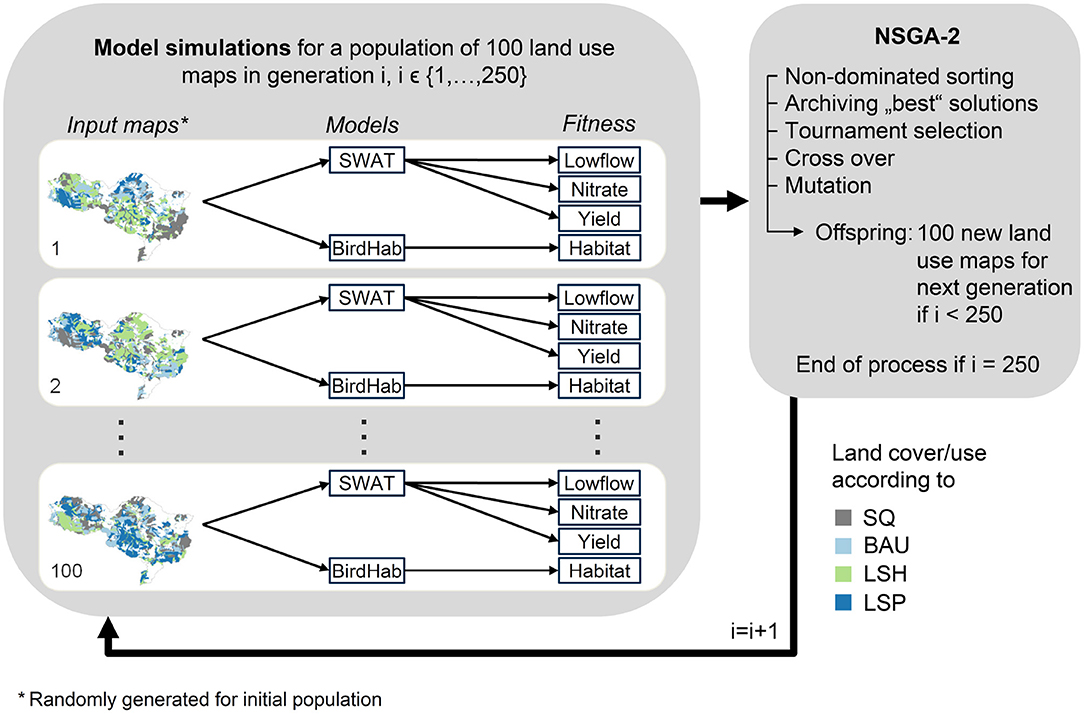
Figure 3. Simplified workflow of the optimization process. CoMOLA starts an evolutionary process by first creating a set of different randomly generated land use maps (n = 100). As the algorithm is inspired by biological evolution, its terminology and principles are likewise: each land use map is called an individual and is represented by a genome, i.e., a string of integers encoding the land use of each Hydrological Response Unit (HRU). Land cover and land use in an HRU can either be represented by scenario SQ (status quo), BAU (business as usual), LSH (land sharing), or LSP (land sparing). All maps of one generation form a population which changes over generations due to selection and variation (i.e., crossover and mutation). Using the Soil and Water Assessment Tool (SWAT) and a Random Forest bird species distribution model (BirdHab), each individual is assigned fitness values representing the achieved values for the four objectives. The genetic algorithm then applies a Pareto ranking for each individual based on its fitness. It archives best individuals and selects individuals for mating to generate a new (offspring) population. In mating, each offspring individual is generated by a random combination (crossover) of two genomes. The likelihood of mating increases for individuals with a higher Pareto rank. Additional random mutations increase the diversity of genomes to consider a wide range of different spatial configurations. The entire procedure, from fitness value calculation to offspring generation, is repeated for 250 generations.
Biodiversity was modeled with a species distribution model that has been developed within the TALE project. A detailed description can be found on the TALE Learning Environment (TALE, 2020) and an example of its application to the Middle Mulde River Basin in Jungandreas et al. (2018). Furthermore, the code and example input data for the Lossa River Basin are provided in a GitHub repository (Jungandreas et al., 2020). This bird habitat model accounts for the impact of the different land management scenarios on 15 Red List bird species (see Supplementary Table 1) by identifying percental changes in suitable habitat compared to the current situation (i.e., SQ). For the status quo, the index value is 1 since it serves as a reference for the evaluation of other landscape settings. If the model returns an index value <1, then suitable habitat decreased, if it is >1, suitable habitat increased.
The optimization problem was solved with the tool CoMOLA (Constrained Multi-objective Optimization of Land Allocation) (Strauch et al., 2019) which applies the non-dominated sorting genetic algorithm II (NSGA-II) (Deb et al., 2002). The result of such a multi-objective optimization is a so-called Pareto-frontier–a set of non-dominated solutions. This means that there is no other feasible solution to the optimization problem that improves one of the objectives without compromising on at least one other objective. The optimization process is summarized in Figure 3. In our case, the algorithm detected 2419 Pareto-optimal solutions that served as input data for our study (Strauch et al., 2018).
2.3. Parallel Coordinates Plots
Each of the above-mentioned solutions consist of a map with a unique spatial distribution of the four land management scenarios that imply different objective function values (also called fitness values). For example, Figure 4 shows the maps of the four extreme solutions, i.e., those scenario distributions that lead to the highest fitness value for each objective, respectively. The solution “water quality,” for instance, has a fitness value of 1.24 for biodiversity, 89.1 l/s for water quantity, 8,149 kg N/a for water quality (the best over all solutions), and 1.95 M €/a for agricultural production, respectively.
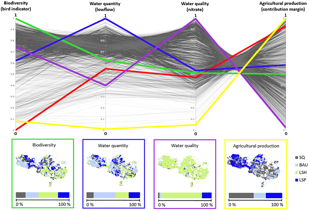
Figure 4. Parallel coordinates plot of the Pareto-optimal solutions. The solutions with the best performance for each objective (extreme solutions) are marked in yellow (contribution margin), green (biodiversity), blue (water quantity), and purple (water quality), the red line corresponds to the status quo. The respective spatial distribution and the percental share of the land management scenarios are shown in the boxes below the plot.
For the stakeholders, we illustrated the optimal solutions with interactive parallel coordinates plots (Figure 4). Each axis stands for one of the four objectives. The solutions are drawn as lines that connect the solution's fitness values (here, normalized values) with each other across these axes. The higher a line is placed within the graph, the better the respective objective values are. For the “water quality” extreme solution this would be the purple line running through the top-most point of the “water quality” axis. As a reference for the stakeholders, we also plotted the status quo line (red). Once we explained the principle of the parallel coordinates plots as mentioned above, we added four extra axes that represented the four scenarios (Supplementary Figure 1). Each solution was illustrated not only by its fitness values but also by its percental distribution of the scenarios (see https://figshare.com/articles/figure/Interactive_parallel_coordinates_plot/13373018 for the interactive version of this plot).
The interactive parallel coordinates plots allowed us to visualize the trade-offs between the different objectives by letting the stakeholders browse through the set of Pareto-optimal solutions. Furthermore, they got an impression of what implications high fitness values for certain objectives may have for the spatial distribution of the scenarios, and thus, land management.
2.4. Analytic Hierarchy Process
To determine the stakeholder's preferences for the four optimization objectives, we used the Analytic Hierarchy Process (AHP) (Saaty, 1988). The method of the AHP is based on pairwise comparisons of all objectives that finally lead to a ranking of the same. According to our four objectives, we had six pairwise comparisons (i.e., objective A vs. objective B). During each comparison, the stakeholder was asked to express his preference on a scale from 1 to 9 (Saaty, 2008), where 1 means that both objectives are equally important and 9 that the respective objective is extremely more important than the other one (see Table 2). For example, the stakeholder was asked: “What is your first preference–water quality or agricultural production–and to what degree?” For the interviews, we used the AHP Excel Template by Goepel (2013). This template also allows for multiple inputs (since we conducted more than one AHP ranking). The individual judgements were consolidated by calculating the weighted geometric mean.
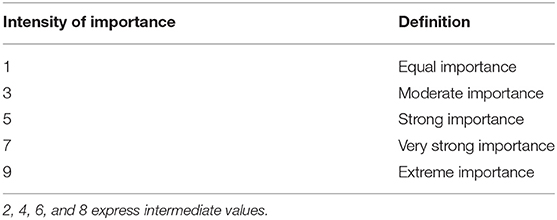
Table 2. Scale of the analytic hierarchy process (AHP) (Saaty, 2008).
2.5. Stakeholder Interviews
The qualitative interviews were conducted in February/March 2019. For these, we selected experts that have a stake in the case study area and represent one or multiple aspects of the above-explained optimization. In total, we interviewed 11 stakeholders with backgrounds in water-related occupations (2), forestry (1), agriculture (3), landscape planning (1), and nature conservation (4) (see Supplementary Table 2 for details).
Each interview started with a presentation that covered a general introduction to land use conflicts, the TALE project and the case study area. Also, important terms, such as “trade-offs,” “synergies,” “land sharing,” and “land sparing” were defined. Then, the interview partner was informed of the different scenarios as described in Table 1 and (very generally) about the optimization process. Great emphasis was put on the explanation and interpretation of the optimization results since they formed the basis of the following evaluation (Step 1 in Figure 1). For this, we used parallel coordinates plots in order to inform the stakeholders about the trade-offs and synergies between the four objectives and their implications on the spatial scenario distribution.
After this introductory block, we started the actual evaluation process using the AHP. During the pairwise comparisons, the stakeholders were provided with information sheets to support their decision-making. For each pairwise comparison, these sheets gave a summary of the trade-offs/synergies between the two objectives in question in terms of a two-dimensional plot of the respective parts of the Pareto frontier. Furthermore, they contained information about scenario distributions (for an example, see Supplementary Figure 2). The stakeholders could also go back to the interactive plots and the scenario definitions. Furthermore, they were asked to give reasons for their decisions while setting their preferences (Figure 1, Step 2).
Following the pairwise comparisons, the stakeholders were shown their individual weights and given the chance to adjust their choices if they were not satisfied with the final weighting.
2.6. Grouping of Stakeholders and Selection of a Preferred Solution
The interviews delivered the individual and overall weighting of the four objectives. However, the different backgrounds were not evenly distributed across the stakeholders. We therefore grouped them into “nature,” “water,” “forest,” “agriculture,” and “landscape planning” (Supplementary Table 2) and calculated the arithmetic mean of all group members' individual weights. These were used to select the best solution of each group but also to identify a best solution over all groups (by again using the arithmetic mean of all group weights).
For the selection of a preferred solution from the Pareto-optimal set, we normalized the fitness values to values between 0 and 1 as follows:
with x being the fitness value that should be normed, min the minimum simulated fitness value of the respective objective, and max the maximum simulated value. The preferred solution was then selected by finding the maximum of the weighted sum of fitness values:
with wi > 0 being the AHP weight of objective i, , and fi the respective normalized fitness value.
We therefore finally got best solutions for (i) the initial overall AHP weights, (ii) the stakeholder groups, and (iii) the overall group weights (Figure 1, Step 3).
3. Results
The results of the AHP over all stakeholders, the stakeholder groups and overall stakeholder groups are provided in Table 3 (individual weights and pairwise comparisons can be found in Supplementary Table 2 and in the Excel file Supplementary Data Sheet 2.xlsx). The stakeholder with a background in landscape planning valued all objectives equally. The result also served as a balanced solution in the further analysis. Apart from that, the majority of the stakeholders considered water quality as being the most important, followed by biodiversity, water quantity, and agricultural production. Two exceptions were the groups “forest” and “agriculture” who valued biodiversity and agricultural production as most important, respectively, and water quality second.
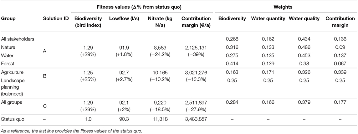
Table 3. The different stakeholder groups, their relative AHP weights for the objective functions and the resulting best solutions with respective objective function fitness values (values in brackets show the percental change from status quo).
By applying the weights to the selection of preferred solutions, some of the groups turned out to have the same best solution. In total, we identified three different solutions that were the best: the preferences of the groups “all stakeholders,” “water,” “nature,” and “forest” lead to solution (A) in Figure 5, those of “landscape planning” (balanced) and “agriculture” to solution (B), and the best solution for all stakeholder group weightings is (C).
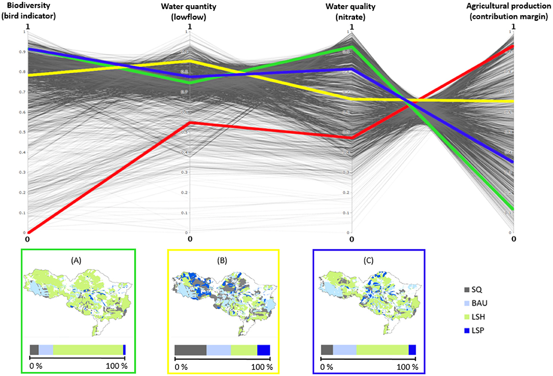
Figure 5. Parallel coordinates plot of the Pareto-optimal solutions with the three AHP best solutions (A)—green line, (B)—yellow line, and (C)—blue line. The red line marks the status quo. The respective spatial distribution and the percental share of the land management scenarios are shown in the boxes below the plot.
The spatial distribution of the land management scenarios varies across those solutions (Figure 5). While solution (A) is dominated by the LSH scenario (73%) and some parts of BAU (15%), solution (B) consists of an almost equal distribution of the scenarios LSH (28%), BAU (26%), and SQ (33%) with a little share of LSP (13%). Solution (C), on the other hand, is somewhat intermediate between (A) and (B) though with a more moderate share of LSH (55%) than (A) and less LSP (7%) and SQ (13%) than (B). All three solutions have in common that there is a large area of BAU in the South-West and of LSH in the North-West. Additionally, scenarios BAU, SQ, and LSP are mainly scattered along the Lossa River. This is particularly visible in solutions (A) and (C) since these have a large share of LSH that dominates the rest of the case study area. However, this does not imply higher rates of fertilization (in fact, fertilizer reduction was highest in these areas because the status quo land use is mainly intensive grassland with highest fertilization rates, see Supplementary Figure 3). In solution (B), all scenarios are rather scattered across the entire river basin though LSH concentrates more in the South-East and LSP and SQ in the central part of the area. Generally, scenario BAU (with the highest increase in urban area, Table 1), was mostly located in close vicinity of existing urban areas and along the road network. Additionally, urban areas had a positive effect on several of the considered bird species since they provide space for nesting, for instance.
These differences also have an effect on the objective performances (in the following, compared to SQ): all objectives improve for all best solutions apart from agricultural production; here, the contribution margin decreases significantly for all of the three solutions. This is partly due to the calculation as a combination of SWAT-simulated crop yields and crop-specific market prices and production costs (Strauch et al., 2018). The contribution margin does not include any subsidies for environmentally friendly farming. Otherwise, the losses might have been less or even fully compensated.
However, some solutions perform better than others for certain objectives: solution (A) has comparatively high fitness values for biodiversity and water quality. Due to the synergy between both objectives, suitable bird habitat increases by up to 29%, and nitrate load can be reduced by 24.2%. Nevertheless, with a loss of 39% in contribution margin, this solution also illustrates the trade-off between biodiversity/water quality and agricultural production. Solution (B), on the other hand, is best for water quantity (though the gain of 2.7% is low compared to the fitness value ranges of the other objectives) and of the three solutions, it has the lowest loss in contribution margin (13.3%). As could be expected, solution (C) is also with respect to the fitness values an intermediate between (A) and (B). All these results are summarized in Table 3.
For all three best solution maps there is almost no change in the actual land use distribution compared to the visible status quo (Supplementary Figure 4). However, there are big changes in land management (Table 4). Solution (A) is the most extensive with the highest increase in conservation tillage, linear elements, and extensive grassland. While solution (B) remains quite intensive with lower reduction in fertilization and a considerably lower increase in extensive grassland and conservation tillage. Solution (C) is, again, an intermediate between (A) and (B).
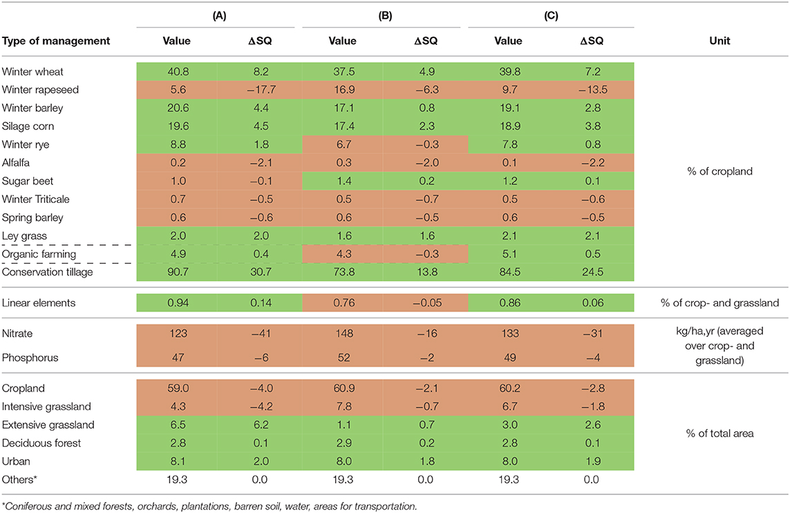
Table 4. Average land management in the Lossa River Basin for best solutions (A), (B), (C), and absolute changes (green: positive and red: negative) compared to status quo (SQ).
The cultivation of winter wheat, winter barley, and corn increases in all three solutions (A, B, and C), as these crops were assumed to be important for all scenarios (BAU, LSH, and LSP), while the more intensive production of winter rapeseed was reduced substantially (highest reduction in A and lowest in B). Overall, there are only small changes in organic farming (as organic farming was assumed to be less relevant for the Lossa Basin, see Table 1); however, conservation tillage is increased and fertilization is reduced for all solutions. In term of land use, extensive grassland (though to very different degrees), forest, and urban areas increase for all three solutions, while cropland and intensive grassland decrease.
4. Discussion
Before we discuss the method presented above, we will first examine the results of the AHP and the emerging best solutions. In this context, the reasons stakeholders gave for their individual preferences will be summarized. We would like to point out that it lies beyond the scope of this paper to discuss details of the optimization process and the scenario development since their results were handled as given and do not have any influence on the framework itself. We will instead focus on the benefits and limitations of the combination of qualitative one-to-one interviews, parallel coordinates plots, and AHP for the selection of preferred solution(s) from a Pareto frontier. Furthermore, we would like to share our experiences with applying this framework in stakeholder interviews.
4.1. Stakeholder Comments
From the four objectives, water quality was the most important for the majority of the stakeholders. The reasons they gave for preferring it over the other objectives during the AHP were mainly that clean water is one of the most basic human needs, and water quality thus directly affects people's lives. Two of the stakeholders also mentioned that in the case study region, there are many areas with deficits in water quality and improving it is thus of high priority. Furthermore, water quality was also rated higher than other objectives because of its strong synergy with biodiversity, which was the second most important objective. When comparing water quality with water quantity, all stakeholders valued water quality as more or at least equally important since, in their opinion, lower levels of water in good quality might be more tolerable than higher levels in poor quality. Nevertheless, water quantity was considered important for the Lossa River Basin, particularly, because it already is a comparatively dry region and a continuous water flow is necessary for maintaining ecological integrity (e.g., supporting the survival of many species) especially in view of drought events that are likely to appear more often with climate change.
When comparing biodiversity with agricultural production, all stakeholders agreed that enhancing and conserving biodiversity is of major importance; some stakeholders even mentioned the positive role of biodiversity for a more sustainable and robust agriculture (e.g., by providing pest control and pollination services—aspects, that were not considered in the optimization). In this context, particularly stakeholders from the “nature” group mentioned that in Germany, agricultural production should rather be reduced and/or extended instead of increased and/or intensified. The farmers agreed that they would accept lower yields if they were compensated for their economic losses. Their main argument in favor of agricultural production was that it is important for their existence. However, the farmers also acknowledged that most of their colleagues have deep roots in their home regions and thus also a vital interest in conserving the surrounding nature and landscape. Additionally, stakeholders mentioned that agriculture is an important factor that shapes the traditional German cultural landscape. Overall, there was a strong consensus among the stakeholders that there should be more support for farmers in order to achieve a more environmentally friendly agricultural production.
4.2. Discussion of Results
The resulting AHP weights that were based on these opinions led to three preferred solutions. The reasons why some stakeholder groups had the same best solution are that either their distribution of weights was similar or because of the synergies between objectives. For example, those stakeholders who valued water quality high (e.g., “nature”) eventually turned out to have the same best solution as those who valued biodiversity high (e.g., “forest”). The impact of the weights on the final preferred solution could be further analyzed by conducting a sensitivity analysis that compares the preferred solutions for stepwise changes in objective function weights. Here, it is most likely the granularity of the Pareto-optimal solutions that plays an important role: if the Pareto-frontier is approximated by only few non-dominated solutions, changes in weights must be greater in order to result in different preferred solutions. The higher the number of non-dominated solutions, therefore, the more likely it is that the preferred solution changes with only little adjustments in weights.
In terms of the spatial land use distributions for the best solutions (A), (B), and (C), most of the cropland patches were not allowed to be converted into another land use, and none of the remaining cropland patches were allowed to be converted into grassland during the optimization (Supplementary Table 3). This explains why there are only little changes in land uses for the three preferred solutions. Scenario LSH dominates on those cropland patches which were forced to remain as such during the optimization which could be understood as a general trend toward an extensification of crop production.
Generally, when interpreting these results, it should be taken into account that the predicted impacts of the different spatial distributions of land use/management on each objective function (biodiversity, agricultural production, water quality, and water quantity) are highly uncertain. We did not provide any uncertainty estimations as the sources of uncertainty are too manifold and difficult to quantify, e.g., input data uncertainty, parameter uncertainty, and especially structural model uncertainty. Nevertheless, most stakeholders were aware of model limitations and did not overestimate single numbers, though they were interested in generic patterns and trends.
4.3. Discussion of the Stakeholder Interviews
Of course, the results of our interviews depend on the selection of stakeholders. Our interview partners had different backgrounds that represented the diverse aspects of the optimization problem. Since the selection was not completely homogeneous across fields, we grouped them and used mean group weights to identify the preferred solutions.
Furthermore, we conducted only 11 interviews. This is due to the fact that we decided for informed expert interviews that took about 1.5–2 h each. Surely, more interviews could have covered a wider range of opinions but would also have exceeded the resources available. Alternatively, the amount of information given before the AHP could be shortened, but we considered it just as important that all stakeholders were fully aware of what effect their preferences would have on land management and objective function performances in our case study area. Additionally, we were interested in the reasons the stakeholders have for their preference selection to enhance the explanation of the results by arguments that cannot be expressed in modeling language. In a one-on-one interview, the stakeholders might be more motivated in giving detailed answers compared to questionnaires where they would have to write them down. Furthermore, the personal dialog gives both sides the opportunity to clarify any questions that may arise, which is very helpful in contexts with complex interrelations, such as land use allocation problems.
The AHP was easy to understand for the stakeholders and the Excel template by Goepel (2013) provided a straightforward way of its implementation. A benefit of applying the AHP in our context is that there is no negotiation necessary between the different stakeholders and each stakeholder's preferences have an equal influence on the final selection of a preferred solution. This might not be the case in workshop discussions since some stakeholders could be more dominant than others. Furthermore, the AHP allows for clustering of the stakeholders, which can be useful for the analysis of common interests/needs and disagreements, particularly in light of future group negotiations.
A difficulty we experienced during the AHP was to make sure that the weightings were consistent. The consistency is expressed in terms of an indicator that is also part of the Excel template by (Goepel, 2013) (see AHPcalc_anonymized.xlsx in the Supplementary Material for the consistency ratios of our interviews). The template also shows those pairwise comparisons that should be adjusted to increase consistency. However, there are usually multiple options to adjust preferences, and the higher the number of pairwise comparisons is the more difficult it gets to identify those that the stakeholder is willing to change and would increase consistency.
A limitation of using the AHP to weigh the objectives is that the resulting land use maps are not necessarily acceptable to the stakeholders. Additionally, it might happen that a selected solution cannot be put into practice. In our interviews, the final weights were presented to each stakeholder who then had the opportunity to adjust the pairwise comparisons if the result did not reflect his/her opinion. However, if they made any at all, the stakeholders did only minor changes. We did not provide them with the final best solution according to their preferences since we informed the stakeholders before the AHP about the trade-offs and synergies. We therefore assumed that they were able to estimate the impact of their weightings on the final solution. Furthermore, individual best solutions were not relevant for our approach as we consolidated the weights to select the preferred solutions over different stakeholder groups.
We are aware that, without testing the acceptability of the individual preferred solutions, there is a risk that individual weights that lead to unfavorable solutions negatively influence the overall group weighting. For further studies, we therefore suggest providing not only the final weights but also the respective preferred solution and objective function values to the interview partner for validation. This can be done on-the-fly since running Equation (2) takes only seconds and maps for each Pareto-optimal solution can be generated before the interviews.
The next step after detecting the overall final preferred solution(s) would be their validation during a stakeholder workshop as indicated in Step 4* in Figure 1. In case the decision makers do not agree with a solution, the weights could be adjusted and a new solution selected. In this context, it is possible to conduct a sensitivity analysis of the AHP weights. This would give information about how and when results change if the stakeholder changes his/her opinion (for an example, see Ayadi et al., 2017). Alternatively, and if only few changes are necessary, the AHP weights could be used as input for a pruning approach. This would mean that the weights serve as an indicator for the area of the Pareto-frontier from which an alternative solution can be selected (i.e., a solution from the neighborhood of the initial preferred solution).
Overall, our framework is based on the assumption that the information (particularly about trade-offs and synergies) given before the AHP has an influence on the stakeholder's preferences. It could be argued that using the AHP weights immediately within the optimization (e.g., a weighted-sum approach) or pruning rules that steer the optimization toward a certain area of the Pareto frontier would be more straightforward since it is not sure to which extent previously given information really has an impact on the stakeholder's decision-making. This is surely an aspect for future research and the influence most likely depends on the type of stakeholder, his/her expertise, and how much background knowledge about the specific research question he/she already had before the interview. It might also be a general question how much and what kind of information is necessary and how it should be presented to ensure its consideration in informed decision-making.
Nevertheless, our approach considers the possibility that previously given information does have an impact on the decision-making, and the quality of the identified solutions does not degrade if this is not the case since we suggest their validation within a stakeholder workshop. Furthermore, it allows us to analyze the entire potential of the landscape and trade-off and synergy relations between the different objectives which would not be possible by applying the above-mentioned alternatives.
4.4. Discussion of Visualization Methods
As mentioned in the Introduction, there are various methods for the visualization of Pareto-optimal solutions. However, only few of them are suitable for a trade-off analysis that uses the entire optimal set, especially when stakeholders are involved. Spider charts, for instance, can become very crowded when displaying a large number of solutions. Furthermore, analyzing the trade-offs across various objectives might be easier if the axes are ordered straight (like in parallel coordinates plots) and not circular.
Hyper-radial visualization (HRV) (Chiu et al., 2009) is a very practical tool for the visualization of the solutions of a many-objective optimization problem. All objectives are arranged into two groups and then, after normalizing and calculating a hyper-radius, the solutions are displayed in a two-dimensional plot. The method can also take into account objective weightings and uncertainties. If the stakeholder preferences are known, HRV can be used for the selection of the best solution. Nevertheless, due to the grouping of objectives, the interpretation of the plot for the analysis of trade-offs between these objectives might be less intuitive for stakeholders compared to other methods.
Decision maps, for instance, display the Pareto frontier in a two-dimensional plot for three and up to seven objectives. The concept of this visualization method is that, for example, in a case of three objective functions, a bi-criterion trade-off curve is constructed, and a constraint on the value of the third objective is imposed on this plot. When different values of the third objective are added to the plot, the result looks very similar to a topographic map. Further objectives can be added with the use of slider bars. In summary, each snapshot of a decision map shows the full feasible range of two objectives while the values of the other objectives are fixed (for a more detailed description of this method we refer to Lotov et al., 2004).
However, decision maps require the calculation of the Edgeworth-Pareto Hull for each objective, which can be realized relatively fast for linear and non-linear convex optimization problems. The calculation for non-linear non-convex problems, which is the case for most land use allocation problems (Kaim et al., 2018), is also possible but more time-consuming (Lotov et al., 2004).
The visualization of trade-offs and synergies between the four objectives with an interactive parallel coordinates plot was considered as comprehensible and very helpful by all stakeholders. They particularly appreciated that the whole range of solutions could be easily analyzed. The visualization of results with maps, on the other hand, was only considered as helpful when giving examples of the spatial scenario distribution of certain solutions (e.g., as we did with the extreme solutions of the optimization results). The stakeholders mentioned that they prefer graphs that illustrate general changes as maps are sometimes difficult to interpret. This is also in line with our experiences from other stakeholder workshops. Therefore, we preferred parallel coordinates plots that furthermore provided the opportunity to directly include the scenario distributions into the trade-off analysis. Nevertheless, for other problem settings, decision maps might be a good alternative.
During the pairwise comparisons of the AHP, the interview partners had the chance to use the parallel coordinates plot to support their decision-making. In doing so, many of them focused mainly on the comparison of trade-offs between the objectives and less on the actual land management changes although they were part of the plot and the stakeholders were provided with a sheet that showed the information given in Table 1. A reason could be that it is difficult to keep an overview over how four objectives and four scenarios interact. Parallel coordinates plots are thus most likely more effective when they consist of a very limited number of axes (Chiu et al., 2009). This is also in line with Lotov et al. (2004) who state that a human being cannot operate more than seven objects.
In summary, the selection of a suitable visualization method for informing stakeholders about the trade-offs and synergies between different objectives depends on the problem at hand and the time that is available for training the stakeholders in interpreting them (Miettinen, 2003). Furthermore, it could also be considered that we offer the stakeholder different forms of visualization from which he or she can select the most illustrative and informative (Miettinen, 2003).
5. Conclusion
We presented a framework that helps selecting one or multiple preferred solution(s) from a Pareto-optimal set of land management allocations considering stakeholder preferences. The framework describes how expert interviews can be conducted, visualizing the solutions from the Pareto-frontier with parallel coordinates plots and identifying objective function weights with the Analytic Hierarchy Process (AHP).
Although the framework was developed for one-on-one expert interviews, it could also be applied to other interview formats like online surveys; for instance, the interactive parallel coordinates plots could easily be integrated into a website and the AHP can handle an unlimited number of participants. This way, the number of interviews could be increased but likely at cost of level of detail [optimal length of a web survey is max. 20 min (Revilla and Ochoa, 2017)] and understanding (the interview partner cannot ask any questions).
For further applications of the framework, we also suggest limiting the number of axes in the parallel coordinates plot. For example, only the objectives could be represented on axes and the scenario distributions (or land use changes in other problem formulations) of each single solution could appear as diagrams (e.g., bar plots) when browsing through the solutions.
This paper provides only one possible way of how the results of a land use allocation problem can be processed for its practical application. In general, future research in land use optimization should always keep in mind how the oftentimes complex results can be visualized comprehensively and appropriately for a non-scientific audience and how they can be embedded into methods that analyze stakeholder preferences as these become more and more important in real-world decision making.
Data Availability Statement
The raw data supporting the conclusions of this article will be made available by the authors, without undue reservation.
Ethics Statement
Ethical review and approval was not required for the study on human participants in accordance with the local legislation and institutional requirements. Written informed consent for participation was not required for this study in accordance with the national legislation and the institutional requirements.
Author Contributions
AK designed the research, conducted the stakeholder interviews, and wrote the manuscript. MS provided the optimization results and assisted with the stakeholder interviews. AK and MS analyzed and interpreted the results of the interviews and the preferred solutions. MS and MV edited the manuscript. All authors contributed to the article and approved the submitted version.
Funding
This research was funded through the 2013/2014 BiodivERsA/FACCE-JPI joint call, with the national funder BMBF-German Federal Ministry of Education and Research (Project TALE-Towards Multifunctional Agricultural Landscapes in Europe: Assessing and governing synergies between food production, biodiversity, and ecosystem services, grant 01 LC 1404 A).
Conflict of Interest
The authors declare that the research was conducted in the absence of any commercial or financial relationships that could be construed as a potential conflict of interest.
Supplementary Material
The Supplementary Material for this article can be found online at: https://www.frontiersin.org/articles/10.3389/frwa.2020.579087/full#supplementary-material
The interactive parallel coordinates plot can be found here: https://figshare.com/articles/figure/Interactive_parallel_coordinates_plot/13373018.
References
Arnold, J. G., and Fohrer, N. (2005). Swat2000: current capabilities and research opportunities in applied watershed modelling. Hydrol. Process. 19, 563–572. doi: 10.1002/hyp.5611
Ayadi, O., Felfel, H., and Masmoudi, F. (2017). Analytic hierarchy process-based approach for selecting a pareto-optimal solution of a multi-objective, multi-site supply-chain planning problem. Eng. Optimiz. 49, 1264–1280. doi: 10.1080/0305215X.2016.1242913
Borges, J. G., Marques, S., Garcia-Gonzalo, J., Rahman, A. U., Bushenkov, V., Sottomayor, M., et al. (2017). A multiple criteria approach for negotiating ecosystem services supply targets and forest owners' programs. For. Sci. 63, 49–61. doi: 10.5849/FS-2016-035
Bouyssou, D. (2001). “Outranking methods,” in Encyclopedia of Optimization, eds C. A. Floudas and P. M. Pardalos (Dordrecht; London: Kluwer Academic), 1919–1925. doi: 10.1007/0-306-48332-7_376
Busch, M., Katzenberger, J., Trautmann, S., Gerlach, B., Dröschmeister, R., and Sudfeldt, C. (2020). Drivers of population change in common farmland birds in germany. Bird Conserv. Int. 117, 1–20. doi: 10.1017/S0959270919000480
Celli, G., Chowdhury, N., Pilo, F., Soma, G. G., Troncia, M., and Gianinoni, I. M. (2018). Multi-criteria analysis for decision making applied to active distribution network planning. Electric Power Syst. Res. 164, 103–111. doi: 10.1016/j.epsr.2018.07.017
Chikumbo, O., Goodman, E., and Deb, K. (2014). Triple bottomline many-objective-based decision making for a land use management problem. J. Multicriteria Decis. Anal. 22, 133–159. doi: 10.1002/mcda.1536
Chiu, P. W., Naim, A. M., Lewis, K. E., and Bloebaum, C. L. (2009). The hyper-radial visualisation method for multi-attribute decision-making under uncertainty. Int. J. Product Dev. 9:4. doi: 10.1504/IJPD.2009.026172
Deb, K., Pratap, A., Agarwal, S., and Meyarivan, T. (2002). A fast and elitist multiobjective genetic algorithm: NSGA-II. IEEE Trans. Evol. Comput. 6, 182–197. doi: 10.1109/4235.996017
European Environment Agency (2018). European Waters: Assessment of Status and Pressures 2018, Volume no 2018, 7 of EEA Report. Luxembourg: Publications Office of the European Union.
Ferreira, J. C., Fonseca, C. M., and Gaspar-Cunha, A. (2008). “Methodology to select solutions from the pareto-optimal set,” in DaMaP 2008, eds A. Doucet, S. Gançarski, and E. Pacitti (New York, NY: ACM Press), 789.
Goepel, K. D. (2013). “Implementing the analytic hierarchy process as a standard method for multi-criteria decision making in corporate enterprises - a new AHP excel template with multiple inputs,” in Proceedings of the 12th International Symposium on the Analytic Hierarchy Process for Multicriteria Decision Making (Kuala Lumpur). doi: 10.13033/isahp.y2013.047
Hagemann, N., van der Zanden, E. H., Willaarts, B. A., Holzkämper, A., Volk, M., Rutz, C., et al. (2020). Bringing the sharing-sparing debate down to the ground–lessons learnt for participatory scenario development. Land Use Policy 91:104262. doi: 10.1016/j.landusepol.2019.104262
Inselberg, A., and Dimsdale, B. (1990). “Parallel coordinates: a tool for visualizing multi-dimensional geometry,” in Proceedings of the 1st Conference on Visualization '90, VIS '90 (Washington, DC: IEEE Computer Society Press), 361–378. doi: 10.1109/VISUAL.1990.146402
Jungandreas, A., Václavík, T., Strauch, M., Cord, A. F., and Volk, M. (2018). Future Land Management Strategies and Their Impact on Breeding Habitats of Endangered Bird Species in Saxony, Germany. Available online at: http://tale.environmentalgeography.nl/wp-content/uploads/2020/03/Gfo2018_JungandreasA.pdf (accessed March 20, 2020).
Kaim, A., Cord, A. F., and Volk, M. (2018). A review of multi-criteria optimization techniques for agricultural land use allocation. Environ. Model. Softw. 105, 79–93. doi: 10.1016/j.envsoft.2018.03.031
Karner, K., Cord, A. F., Hagemann, N., Hernandez-Mora, N., Holzkämper, A., Jeangros, B., et al. (2019). Developing stakeholder-driven scenarios on land sharing and land sparing-insights from five european case studies. J. Environ. Manag. 241, 488–500. doi: 10.1016/j.jenvman.2019.03.050
Kollat, J. B., and Reed, P. (2007). A framework for visually interactive decision-making and design using evolutionary multi-objective optimization (video). Environ. Model. Softw. 22, 1691–1704. doi: 10.1016/j.envsoft.2007.02.001
Lautenbach, S., Volk, M., Strauch, M., Whittaker, G., and Seppelt, R. (2013). Optimization-based trade-off analysis of biodiesel crop production for managing an agricultural catchment. Environ. Model. Softw. 48, 98–112. doi: 10.1016/j.envsoft.2013.06.006
Li, Z., Liao, H., and Coit, D. W. (2009). A two-stage approach for multi-objective decision making with applications to system reliability optimization. Reliabil. Eng. Syst. Saf. 94, 1585–1592. doi: 10.1016/j.ress.2009.02.022
Lotov, A. V., Bushenkov, V. A., and Kamenev, G. K. (2004). Interactive Decision Maps: Approximation and Visualization of Pareto Frontier, Volume 89 of Applied Optimization. Boston, MA: Springer US.
Lotov, A. V., and Miettinen, K. (2008). “Visualizing the pareto frontier,” in Multiobjective Optimization, Lecture Notes in Computer Science, ed J. Branke (Berlin: Springer), 213–243. doi: 10.1007/978-3-540-88908-3_9
Marto, M., Reynolds, K., Borges, J., Bushenkov, V., and Marques, S. (2018). Combining decision support approaches for optimizing the selection of bundles of ecosystem services. Forests 9:438. doi: 10.3390/f9070438
Memmah, M.-M., Lescourret, F., Yao, X., and Lavigne, C. (2015). Metaheuristics for agricultural land use optimization. A review. Agron. Sustain. Dev. 35, 975–998. doi: 10.1007/s13593-015-0303-4
Miettinen, K. (2003). “Graphical illustration of pareto optimal solutions,” in Multi-Objective Programming and Goal Programming, Vol. 10, eds T. Tanino, T. Tanaka, and M. Inuiguchi (Berlin; Heidelberg: Springer Berlin Heidelberg), 197–202. doi: 10.1007/978-3-540-36510-5_27
Miettinen, K. (2014). Survey of methods to visualize alternatives in multiple criteria decision making problems. OR Spectrum 36, 3–37. doi: 10.1007/s00291-012-0297-0
Miettinen, K., Molina, J., González, M., Hernández-Díaz, A., and Caballero, R. (2009). Using box indices in supporting comparison in multiobjective optimization. Eur. J. Oper. Res. 197, 17–24. doi: 10.1016/j.ejor.2008.05.013
Ojha, A., Das, B., Mondal, S., and Maiti, M. (2010). A stochastic discounted multi-objective solid transportation problem for breakable items using analytical hierarchy process. Appl. Math. Model. 34, 2256–2271. doi: 10.1016/j.apm.2009.10.034
Revilla, M., and Ochoa, C. (2017). Ideal and maximum length for a web survey. Int. J. Market Res. 59, 557–565. doi: 10.2501/IJMR-2017-039
Saaty, T. L. (1988). Multicriteria Decision Making: The Analytic Hierarchy Process; Planning, Priority Setting, Resource Allocation, Volume 1 of The Analytic Hierarchy Process Series. 2nd Edn. New York, NY: McGraw-Hill.
Saaty, T. L. (2008). Decision making with the analytic hierarchy process. Int. J. Serv. Sci. 1, 83–98. doi: 10.1504/IJSSCI.2008.017590
Strauch, M., Cord, A. F., Pätzold, C., Lautenbach, S., Kaim, A., Schweitzer, C., et al. (2019). Constraints in multi-objective optimization of land use allocation-repair or penalize? Environ. Model. Softw. 118, 241–251. doi: 10.1016/j.envsoft.2019.05.003
Strauch, M., Schönhart, M., and Volk, M. (2018). Policy Options to Reconcile Food Production, Biodiversity and Ecosystem Service Provision. Deliverable 4.1, BiodivERSsA-Project TALE.
TALE (2020). Towards Multifunctional Agricultural Landscapes in Europe: TALE Learning Environment. Available online at: http://tale.environmentalgeography.nl/ (accessed March 3, 2020).
Wismans, L. J., Brands, T., van Berkum, E. C., and Bliemer, M. C. (2014). Pruning and ranking the pareto optimal set, application for the dynamic multi-objective network design problem. J. Adv. Transport. 48, 588–607. doi: 10.1002/atr.1212
Keywords: land use allocation, multi-objective optimization, trade-off visualization, stakeholder communication, preferences, analytic hierarchy process
Citation: Kaim A, Strauch M and Volk M (2020) Using Stakeholder Preferences to Identify Optimal Land Use Configurations. Front. Water 2:579087. doi: 10.3389/frwa.2020.579087
Received: 01 July 2020; Accepted: 17 November 2020;
Published: 22 December 2020.
Edited by:
Dipankar Dwivedi, Lawrence Berkeley National Laboratory, United StatesReviewed by:
Jose G. Borges, University of Lisbon, PortugalJoseph Guillaume, Australian National University, Australia
Raghavendra Belur Jana, Skolkovo Institute of Science and Technology, Russia
Copyright © 2020 Kaim, Strauch and Volk. This is an open-access article distributed under the terms of the Creative Commons Attribution License (CC BY). The use, distribution or reproduction in other forums is permitted, provided the original author(s) and the copyright owner(s) are credited and that the original publication in this journal is cited, in accordance with accepted academic practice. No use, distribution or reproduction is permitted which does not comply with these terms.
*Correspondence: Andrea Kaim, andrea.kaim@uni-bayreuth.de