

Abstract
Most studies assessing climate impacts on agriculture have focused on average changes in market-mediated responses (e.g. changes in land use, production, and consumption). However, the response of global agricultural markets to interannual variability (IAV) in climate and biophysical shocks is poorly understood and not well represented in global economic models. Here we show a strong transmission of IAVs in climate-induced biophysical yield shocks to agriculture markets, which is further magnified by endogenous market fluctuations generated due to producers' imperfect expectations of market and weather conditions. We demonstrate that the volatility of crop prices and consumption could be significantly underestimated (i.e. on average by 55% and 41%, respectively) by assuming perfect foresight, a standard assumption in the economic equilibrium modeling, compared with the relatively more realistic adaptive expectations. We also find heterogeneity in IAV across crops and regions, which is considerably mediated by international trade. Studying IAV provides fundamentally new insights on measuring and understanding climate impacts on global agriculture, and our framework lays the foundation for further investigating the full range of climate impacts on biophysical and human systems.
Export citation and abstract BibTeX RIS
1. Introduction
Climate is essentially an indirect input to agricultural production, and its economic impacts on agriculture have been extensively assessed in the past three decades (Rosenzweig and Parry 1994, Costinot et al 2016, Zhao et al 2020, Gouel and Laborde 2021). The assessment requires a combined use of climate, crop, and economic models to translate climate and biophysical shocks to changes in economic variables such as agricultural production, price, and land use (Nelson et al 2014, Wiebe et al 2015). With the advances in the understanding of the biophysical consequences of changes in temperature, precipitation, and other climate variables on agriculture (Challinor et al 2014, Rosenzweig et al 2014, Frieler et al 2017a), studies are shifting focus from mean to the variability of future climate and biophysical shocks (Huntingford et al 2013, Ray et al 2015, Iizumi and Ramankutty 2016, Waldhoff et al 2020). Interannual variability (IAV), in particular, is an important characteristic of climate and biophysical shocks. However, how IAVs in climate and biophysical shocks are transformed and transferred to global agricultural markets has been largely overlooked (Urban et al 2012).
Previous studies focused on assessing the economic consequences of climate impacts in few future periods (e.g. 2050 or 2100), as most economic models were designed for mid- or long-term projections (e.g. recursive or comparative static models) 1 . As a result, the estimated climate impacts represent cumulative impacts, or interannual mean impacts, relative to a base year. For example, the agricultural model inter-comparison and improvement project (AgMIP) assessments reported global climate impacts (relative to a reference scenario of no climate impacts) of 17% reduction in biophysical yield, 20% higher in producer prices, and 3% decrease in consumption, by 2050 relative to the base year of 2005 2 (see Nelson et al (2014) for model and scenario details). The cumulative estimates imply the interannual mean impacts of about 0.4% reduction in biophysical yield, 0.4% higher in producer prices, and less than 0.1% decrease in consumption across the 45 year study period. More importantly, perfect foresight has been a standard assumption used in economic modeling even though its lack of realism has been criticized (Féménia and Gohin 2011, Calvin et al 2017). With perfect foresight, agricultural producers can perfectly predict future climate and market information and make adaptations accordingly and immediately (e.g. adjusting land use and management practices to compensate for changes in productivity). Nevertheless, for understanding dynamics in the agricultural market, it is undisputed that farmers make suboptimal decisions due to the time lag between planting and harvesting. In reality, farmers make production, land allocation, and management decisions based on their expectations of future yield and prices. As a result, erroneous expectations of prices and yield due to imperfect foresight could undermine the market equilibrium and, thus, generate 'endogenous' market fluctuations (Gouel 2012) in addition to the variation stemmed from exogenous climate and biophysical shocks. The assumption of perfect foresight, ignoring the endogenous market fluctuations, may lead to misleading assessments of the IAV of agricultural economic responses (Mitra and Boussard 2012).
Understanding the IAV of the climate impacts on agricultural economics is crucial to formulating agricultural policies that facilitate agricultural adaptation and maintain food security since changes in the variability of climate and weather patterns will have considerable consequences on agricultural production and market fluctuation (Thornton et al 2014). In this work, we quantify the IAV of climate impacts on agriculture by incorporating adaptive expectations (Nerlove 1958) of annual prices and yield into a well-established global economic model, the global change analysis model (GCAM). That is, agricultural producers make production and land allocation decisions at planting time based on their expectations of prices and yield at harvesting time and adaptively adjust their future expectations with new information. In contrast to perfect foresight, adaptive expectation offers an intuitive and effective approach to characterize the 'endogenous' market fluctuations in agricultural market equilibrium modeling (Féménia and Gohin 2011). Furthermore, we rely on biophysical yield projections estimated from combinations of two climate models, HadGEM2-ES and GFDL-ESM2M and two crop models, EPIC and LPJ-GUESS under representative concentration pathway (RCP) 8.5. We study the impacts of natural climate-induced biophysical yield shocks on agricultural economics to mid-century and assess both mean and IAV of the climate impacts. Our results demonstrate that studying IAV provides fundamentally new insights on measuring and understanding climate impacts on global agriculture.
2. Methods
The modeling chain of assessing climate impacts on agriculture is shown in figure 1. For this study, we modify GCAM v5.1 (Calvin et al 2019) from 5 years to annual time steps and incorporate adaptive expectation into the model. In this section, we describe the model and the coupled scenarios and present the method of quantifying IAV. More detailed information can be found in supplementary information (SI) section S1.1 (available online at stacks.iop.org/ERL/16/104037/mmedia).
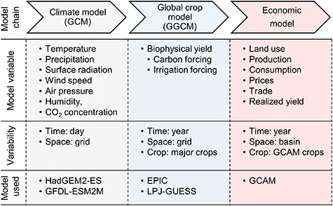
Figure 1. Modeling chain of assessing climate impacts on agriculture. The crop mapping between GGCMs and GCAM is provided in SI table S2.
Download figure:
Standard image High-resolution image2.1. GCAM
GCAM is a dynamic recursive model that represents the linkages between the energy system, water, agriculture and land use, the economy, and the climate. The model has been involved in the AgMIP (Nelson et al 2014, von Lampe et al 2014) and widely used for studying climate impacts on agriculture and land use (Thomson et al 2011, Kyle et al 2014). GCAM with the incorporation of regional agricultural markets is employed in this study. There are 14 crops in GCAM, including 12 food or fiber crops aggregated from FAO crops (see the mapping in table S1) and two dedicated biomass energy crops. The model is global in scope and aggregates the world into 31 regions. The base calibration year is 2010. That is, the model and its database represent the technology, factor productivity, socioeconomic conditions, and market equilibrium in 2010. The GCAM reference scenario uses population and GDP projected in the SSP2, 'Middle-of-the-Road', scenario (O'Neill et al 2014, Samir and Lutz 2017). For biophysical yield growth in the GCAM reference scenario, we use a linear interpolation based on the Food and Agriculture Organization (FAO) of yield projections in 2030 and 2050 (Alexandratos et al 2006, Bruinsma 2009), which represent a trend of total factor productivity (TFP) improvement. The GCAM data system is written in an open-source R package (Bond-Lamberty et al 2019). Both the GCAM model and the data system are publicly available. GCAM, by default, runs to 2100 with 5 year steps. For this study, the model is modified to run in annual time steps to 2050 using external drivers in the reference scenario. A more detailed description of GCAM is provided in SI section S1.2.
For this study, we make modifications in the nested logit land allocation framework in GCAM to incorporate adaptive expectations of prices and yield into the model. It is assumed that a representative profit-maximizing agricultural producer of output  makes production and management decisions by determining the uses of land, water, fertilizer, and other inputs, given a vector of input and output prices and a technology that is constant return to scale. Instead of perfectly predicting prices and yield, agricultural producers form the expectations of the output price (
 ) and yield (
 ) based on existing information. Denote
  ,
,  , and
, and  , as the price for water, fertilizer, and other inputs, respectively and
  ,
,  , and
, and  as the output yield regarding water, fertilizer, and other inputs, respectively. The expected rental profit,
  , earned from land use
  using irrigation option
  (irrigation or rainfed) and fertilizer technology
  (high or low fertilizer) for producers in water basin
  , region
  , and period
  can be derived from the zero pure profit condition, as shown in equation (1).
Note that  ,
,  , and
, and  are input cost per unit output of
  for water, fertilizer, and other inputs, respectively. If farmers have perfect foresight on market prices and yield, i.e.
  and
and  , equation (1) becomes the rental profit used in the original GCAM. Note that incorporating yield expectations (
 ) at the technology level allows further reflecting suboptimal management decisions so that endogenous yield responses, modeled as technology transitions through land use change, could be imperfect. We employ the Nerlove adaptive expectation (equation (2)), which has been extensively studied in the literature (Pashigian 1970, Hommes 1992, 1994) and also explored in recent studies (Féménia and Gohin 2011, Mitra and Boussard 2012, Chaudhry and Miranda 2018). It depicts that the expectation of a variable (
 ) is adaptively revised in proportion to the difference between the previous observation (
 ) and the previous expectation (
 ) with a constant coefficient of expectations (
 ), and
 ![$\alpha \in \left( {0,{\text{ }}1} \right]$](https://content.cld.iop.org/journals/1748-9326/16/10/104037/revision2/erlac2965ieqn28.gif) .
.

Equation (2) can be rearranged to  , which implies that the current expectation is a weighted average of the lagged observation and the lagged expectation. It collapsed into a naïve expectation when
  equals one. In line with previous studies (Boussard et al
2006, Féménia and Gohin 2011), we use a relatively small coefficient of expectation, i.e.
equals one. In line with previous studies (Boussard et al
2006, Féménia and Gohin 2011), we use a relatively small coefficient of expectation, i.e.  , to avoid unrealistic bifurcation or chaotic oscillations (Gouel 2012), and a uniform value is used for all regions and crops. We also test the sensitivity of the IAV of climate impacts on agriculture to
  with a range of [0.05, 0.2]. Further details of expectation schemes and discussions of parameters are provided in SI section S2.
2.2. Climate and baseline scenarios
In this study, we rely on future climate scenarios of biophysical yields estimated in the context of the inter-sectoral impact model intercomparison project (ISIMIP) (Warszawski et al 2014) and the AgMIP. We employ the results from the combinations of two global gridded crop models (GGCMs), EPIC (Kiniry et al 1995, Izaurralde et al 2006) and LPJ-GUESS (Smith et al 2014) and two general circulation models (GCMs), HadGEM2-ES and GFDL-ESM2M. We focus on RCP 8.5 (540 ppm CO2 concentration in 2050) and allow carbon fertilization. The climate and agronomic scenarios have been widely used in previous studies (Nelson et al 2014, Springmann et al 2016), and they are at the extremes (high and low ends at the global aggregated estimates) in their respective model intercomparisons (Rosenzweig et al 2014, Warszawski et al 2014). Thus, there are four climate scenarios evaluated in our study: HadGEM2-ES and EPIC (HE), GFDL-ESM2M and EPIC (GE), HadGEM2-ES and LPJ-GUESS (HL), and GFDL-ESM2M ES and LPJ-GUESS (GL). Future biophysical crop yield shocks reported by crop models are mapped and aggregated to GCAM crops (table S2) following methods developed in Snyder et al (2020) and Müller and Robertson (2014).
The GCAM reference scenario, i.e. no climate impacts but with imperfect foresight, is used as the baseline in this study. Note that the only difference between climate scenarios and the baseline scenario is the external driver of biophysical yield. The biophysical yield by 2050 in the reference and climate scenarios are compared in SI figures S1 and S2. The reference scenario uses a linear interpolation of the FAO projections of crop yield in 2030 and 2050, which implies a trend of TFP growth and does not account for climate variations. The world average biophysical yield in the climate scenarios is projected to be about 5% (GL) to 24% (HE) lower than reference by 2050 relative to 2010 3 . It is important to note that projections in climate scenarios are constructed by applying biophysical yield shocks to the reference GCAM projections following the AgMIP convention (Müller and Robertson 2014, Nelson et al 2014). In other words, the biophysical yield projections in climate scenarios provide an agronomic representation of climate variables on top of a linear trend of TFP growth. Note that the variability in biophysical yield in climate scenarios, when detrended by the TFP trend in baseline, mirrors only the natural climate variability implied by variables in climate models, e.g. temperature, precipitation, surface radiation, wind speed, air pressure, humidity (see discussions in SI section S1.3).
2.3. Climate impact and IAV
We estimate climate impacts on agricultural economic variables in a future year as the relative ratio between a climate scenario and the baseline scenario (no climate impacts), i.e.  . The ratio is compared to one (i.e.
  ), implying a temporally cumulative measure of impacts, and climate impacts on a variable in year,
  , relative to a base year can be calculated as
  (Nelson et al
2014). Note that the corresponding interannual climate impacts can be calculated as
(Nelson et al
2014). Note that the corresponding interannual climate impacts can be calculated as  . However, in this study, we employ the logarithmic changes of cumulative impacts,
  , to measure interannual climate impacts. Using logarithmic changes, implying continuously compounded growth rates, permits a consistent measure of the IAV of climate impacts as the standard deviation of the interannual climate impacts, i.e.
 ![${\text{IAV}} = {\text{SD}}\left[ {\log \left( {{S_t}} \right) - \log \left( {{S_{t - 1}}} \right)} \right]$](https://content.cld.iop.org/journals/1748-9326/16/10/104037/revision2/erlac2965ieqn39.gif) , which has been widely used for measuring market variability (Gilbert and Morgan 2010, Haile et al
2015). It also allows a consistent comparison across climate scenarios for interannual climate impacts when the same baseline scenario is used, i.e.
, which has been widely used for measuring market variability (Gilbert and Morgan 2010, Haile et al
2015). It also allows a consistent comparison across climate scenarios for interannual climate impacts when the same baseline scenario is used, i.e.  , and for IAV when the baseline variability is small (e.g. linear TFP growth in GCAM baseline).
Furthermore, we define relative interannual variability (RIV), as the ratio of the IAV of economic responses ( ) to the IAV of biophysical yield shocks (
 ), i.e.
  . RIV normalizes IAV by biophysical yield so that it can be compared across scenarios, regions, or crops. More importantly, RIV enhances the explanation of the results since it can be decomposed as the ratio of beta coefficient to the correlation coefficient, both between economic responses and biophysical yield shocks, i.e.
  . Beta coefficient implies the magnitude of the interannual economics responses against climate impacts on biophysical yield, and correlation coefficient indicates the extent to which IAV in economic responses is explained by biophysical variability.
3. Results
3.1. Climate impacts on global agriculture to mid-century
Figure 2 presents a time-series (annual) evaluation of agricultural economic responses to climate-induced biophysical shocks by mid-century, under the assumption of adaptive expectations. Note that point estimating of the climate impacts by the year 2050 will also indicate the interannual mean impacts over the study period (see density bars in figure 2 top panels). On average across climate scenarios, regions, and crops, by 2050, biophysical yield is estimated to decrease by 11.2%. It results in higher agricultural area expansion (+7.8%) and yield intensification (+0.5%), which alleviate some of the effects of climate impacts on production. Specifically, production only declines by 4.3% despite the higher decline in yield. The negative impact on crop supply leads to significantly higher crop prices (+36%) and lower consumption (−6%). The average impact on consumption tends to be higher than production due to the higher average impact on export (+24%) relative to import (+13%). The strong regional heterogeneity in biophysical yield shocks alters comparative advantage across the regions. As a result, trade patterns change, with small exporters being more responsive. In addition, scenarios with relatively stronger impacts on biophysical yield (i.e. HadGEM2-ES and EPIC scenarios) show more severe climate impacts on the agricultural market by mid-century. These mean climate impact results are generally consistent with previous studies (Nelson et al 2014), as the expectation scheme has a fairly small influence on the mean impacts (SI section S3.1).
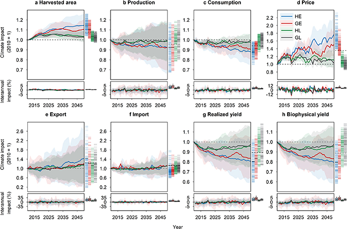
Figure 2. Climate impacts on global agriculture to mid-century. Cumulative (top panels) and interannual (bottom panels) climate impacts on agricultural crop harvested area (a), production (b), consumption (c), price (d), export (e), import (f), realized yield (g) and biophysical yield (h) relative to the GCAM reference scenario, estimated under adaptive expectations. Note that realized yield are results from the model after considering endogenous yield responses. Curves and shadows denote average and 10–90 percentile ranges of GCAM results across all crop-region combinations (biomass and fodder crops not included), respectively. Climate scenarios (two climate models by two crop models under RCP8.5 and with carbon fertilization), distinguished by color, include HadGEM2-ES and EPIC (HE), GFDL-ESM2M and EPIC (GE), HadGEM2-ES and LPJ-GUESS (HL), and GFDL-ESM2M ES and LPJ-GUESS (GL). The density bars next to plots of cumulative change show heterogeneity across crop-region values in 2050 for the four climate scenarios (with corresponding shadow colors), with the crop-region average in each scenario (solid black lines) and scenario-average (dotted black line) highlighted. Interannual impact (bottom panels) is calculated as logarithmic changes of cumulative impact (top panels). The boxplot next to plots of interannual impact presents the mean values (points), the median values (line), the 1st and 3rd quartiles (boxes), and the 10–90 percentile ranges (whiskers) of the standard deviations of interannual impact (i.e. IAV) across GCAM crop-region combinations. See SI table S3 for summary statistics and SI figure S7 for sensitivity of IAV to the coefficient of expectation. Data source: GCAM simulation results.
Download figure:
Standard image High-resolution imageWe use the standard deviation of logarithmic interannual changes to measure the IAV of climate impacts (boxplot in figure 2 bottom panels; see SI table S3 for summary statics and SI figure S7 for the sensitivity of IAV to the coefficient of expectation). On average, across climate scenarios, regions, and crops, the IAV of biophysical yield shocks is about 3.05%, which is largely mirrored in the production responses (3.08%). The average IAV of harvested area responses (0.55%) is fairly small as acreage responses are relatively rigid, especially with planting and harvesting decisions separated. The average IAV of crop consumption (2.10%), as mediated by trade and crop substitutions, is considerably smaller than production. Price volatility has been an important characteristic in the agricultural crop market. The average IAV of price responses is 6.33%, which is more than double the average IAV of biophysical yield shocks. Similar to the mean impact, scenarios with higher IAV in biophysical yield shocks also show higher IAV in the economic responses. However, the mean and IAV of climate impacts are separate measurements, which is important when comparing scenarios. For example, EPIC scenarios have higher impacts in both mean and IAV compared with LPJ-GUESS scenarios, while GFDL scenarios show lower mean impacts but significantly higher IAV compared with HadGEM2-ES scenarios.
Our results demonstrate that climate variables are the major sources of variability across time, while agronomic and economic responses contribute relatively more to variability across regions and crops. This is supported by the analysis of variance (ANOVA) conducted for comparing the relative contribution of variation to climate impacts across five factors, i.e. climate model, crop model, region, year, and crop, and their interactions (table 1). For the variability of climate impacts on biophysical yield and economic variables within climate and crop scenarios, year is a significantly more important contributor compared with region and crop, implying relatively higher overall variations across time. When comparing across scenarios, GGCM appears to contribute more to the overall variation. However, when it comes to IAV, the GCM plays a more important role, as implied by the higher interaction with year compared with crop model in the ANOVA (i.e. GCM:year vs GGCM:year).
Table 1. ANOVA for biophysical yield and economic variables. ANOVA is performed for variables and climate scenarios presented in figure 2 across five factors, i.e. climate model (GCM), crop model (GGCM), region, year, and crop, and their interactions. All variables have the same degrees of freedom (Df) across sources presented. The root mean square (RMS), calculated as the square root of Df weighted sum of squares, is used to measure relative contributions of variation. The full ANOVA results with more interactions are presented in SI table S4.
| Source of variation | Harvested area | Production | Consumption | Price | Export | Import | Realized yield | Biophysical yield | |
|---|---|---|---|---|---|---|---|---|---|
| Df | RMS | RMS | RMS | RMS | RMS | RMS | RMS | RMS | |
| GCM | 1 | 6*** | 3 | 7*** | 31*** | 9 | 8 | 9*** | 10*** |
| GGCM | 1 | 24*** | 23*** | 29*** | 114*** | 19 | 23** | 46*** | 48*** |
| Region | 30 | 2*** | 12*** | 2 | 12*** | 56*** | 27*** | 12*** | 13*** |
| Year | 39 | 11*** | 21*** | 24*** | 115*** | 73*** | 55*** | 22*** | 23*** |
| Crop | 9 | 5*** | 10*** | 8*** | 10*** | 32*** | 13* | 10*** | 10*** |
| GCM:region | 30 | 1*** | 3** | 1 | 2 | 13 | 5 | 3** | 3** |
| GCM:year | 39 | 7*** | 17*** | 20*** | 101*** | 80*** | 64*** | 16*** | 16*** |
| GCM:crop | 9 | 1*** | 2 | 2 | 4 | 5 | 5 | 1 | 1 |
| GGCM:region | 30 | 2*** | 4*** | 1 | 5*** | 25*** | 13*** | 4*** | 4*** |
| GGCM:year | 39 | 3*** | 9*** | 9*** | 41*** | 34*** | 34*** | 9*** | 9*** |
| GGCM:crop | 9 | 4*** | 4* | 4*** | 7*** | 15 | 12* | 5*** | 5*** |
The point (.), single asterisk (*), double asterisk (**), and triple asterisk (***) indicate significance levels of 10%, 5%, 1%, and 0.1%, respectively, from the F test.
3.2. The role of expectation scheme in assessing climate impacts on agriculture
How farmers form expectations of market and weather conditions plays a key role in making decisions and adapting to a changing climate. We investigate the role of expectation schemes in modeling climate impacts on agricultural markets by comparing the adaptive expectation with the perfect foresight (see figure 3 for results from the GE scenario). This comparison indicates the degree to which previous studies using perfect foresight have underestimated the economic responses to climate variability since adaptive expectations is a relatively more realistic representation of farmer behavior. Conversely, such comparisons also provide insights on to what extent climate impacts can be alleviated by improving farmers' predictions of prices and yield. The expectation scheme has a relatively small influence on assessing the mean climate impacts, while its influence on the IAV of economic responses is considerable. With perfect foresight, the average IAV (across climate scenarios, regions, and crops) of harvested area increased by a factor of 2.3 compared with adaptive expectation as adaptations through land use change become more responsive to climate variability with perfect expectations. However, the average IAV of price decreases by 55% with perfect foresight, which reflects the magnitude of endogenous market fluctuations generated under adaptive expectation. In other words, the variation in real shocks of biophysical yield, when transferring to market prices, was magnified (by an average factor of 2.2) due to endogenous market fluctuations. With no endogenous market fluctuations, the average IAV of production (−5%), consumption (−41%), and trade (−25% for export and −29% for import) would also decrease compared with adaptive expectation. Consumption is more sensitive to the expectation scheme than production since consumption is more responsive to prices while production is more responsive to biophysical yield shocks. Furthermore, trade responses become relatively less pronounced under perfect foresight as adaptations through land use change, and intensification are more accessible compared with adaptive expectations. These results are consistent across scenarios (see SI figures S3–S5 and table S5) that assuming perfect foresight would underestimate market volatility. They also imply that the volatility of prices and consumption induced by climate impacts can be reduced if farmers can improve their expectations.

Figure 3. The role of expectation scheme in assessing climate impacts on global agriculture to mid-century. Cumulative (top panels) and interannual (bottom panels) climate impacts on agricultural crop harvested area (a), production (b), consumption (c), price (d), export (e), import (f), realized yield (g) and biophysical yield (h) relative to the GCAM reference scenario. Curves and shadows denote average and 10–90 percentile ranges of GCAM results across all crop-region combinations (biomass and fodder crops not included), respectively. Adaptive expectation (default) is compared with perfect foresight using the GFDL-ESM2M and EPIC (GE) scenario. The density bars next to plots of cumulative change show heterogeneity across crop-region values in 2050 for the two expectation schemes (distinguished by color). The boxplot next to plots of interannual change presents the mean values (points), the median values (line), the 1st and 3rd quartiles (boxes), and the 10–90 percentile ranges (whiskers) of the standard deviations of interannual impact (IAV) across GCAM crop-region combinations. Note that biophysical yield shocks are external drivers in the model so that they are not affected by expectation schemes. Results for other climate scenarios are provided in SI figures S3–S5. See SI table S5 for summary statistics and SI figure S7 for sensitivity of IAV to the coefficient of expectation. Data source: GCAM simulation results.
Download figure:
Standard image High-resolution image3.3. Interannual economic responses to biophysical yield shocks
To illustrate how IAV is transferred from biophysical shocks to economic variables, we calculate RIV between economic responses and biophysical yield shocks, which measures the magnitude of the variance transmission. As described in section 2.3, RIV can be decomposed into a ratio between (a) the magnitude of the interannual economic responses against biophysical yield shocks (measured by the beta coefficient, see y-axis in figure 4)) and (b) the correlation coefficient between economic responses and biophysical yield shocks (x-axis in figure 4). That is, the slope of the lines presented in figure 4 represents the average RIV across crop-regions and scenarios, respectively for adaptive expectation (figure 4(a)) and perfect foresight (figure 4(b)). With adaptive expectations, the results show harvested area and consumption are less responsive to interannual biophysical shocks (i.e. absolute beta coefficient smaller than one) in most crop-regions, compared with production, price, or trade. The magnitude of the economic responses is different across economic variables since the climate and biophysical shocks were transferred to economic variables through different market-mediated responses, e.g. land reallocation, yield intensification, trade responses, and substitutions in consumption in the economic system. The correlation analysis indicates that, under adaptive expectation, biophysical yield shocks explain more IAV in crop supply responses (i.e. an R-squared of, on average, 92% for production and 67% for export) but less in price and demand responses (i.e. an R-squared of, on average, 36%, 33%, and 31% for price, import, and consumption, respectively). That is, the correlation between biophysical yield shocks and the economic responses is weaker when the climate variability is transferred from supply to demand variables. Thus, the relatively stronger interannual responses to biophysical shocks along with relatively larger shares of unexplained variations by biophysical shocks determined the more pronounced variance transmission from climate and biophysical variables to prices (with an average RIV of 2.8), under adaptive expectation, compared with other variables.
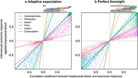
Figure 4. Interannual economic responses and correlations to biophysical yield shocks. The beta coefficient and correlation coefficient between economic variables (distinguished by color) and biophysical yield are presented. Each point denotes a crop in a region and a climate scenario, and only crop-regions in 10–90 percentile ranges of IAV in a climate scenario are presented. Beta coefficients are truncated to [−1, 1] (see SI figure S8 for the figure with full ranges of beta). Note that the relative IAV between economic variables and biophysical yield (ratio of standard deviations) is equal to the ratio of beta coefficient to the correlation coefficient. The slope of the lines represents the average RIV between economic variables and biophysical yield. The black dotted line has a slope of one. The boxplot attached above presents the mean values (points), the median values (line), the 1st and 3rd quartiles (boxes), and the 10–90 percentile ranges (whiskers) of the squares of correlation coefficient, namely coefficient of determination (R-squared). Data source: GCAM simulation results.
Download figure:
Standard image High-resolution imageArea responses, however, only obtained about a quarter of variations in biophysical shocks (RIV is 0.25 on average) under adaptive expectations. Due to the lag between planting and harvesting under adaptive expectations, farmers cannot immediately respond to changes in biophysical shocks by reallocating land, dampening both area responses and its correlation with biophysical shocks. When farmers can adapt immediately (or make better predictions) with perfect foresight (figure 4(b)), increases in the magnitude of area responses are larger than the correlation increases so that higher variations in biophysical shocks are transferred to area responses (RIV increases to 0.54 on average). Also, the stronger land reallocation and intensification responses under perfect foresight reduce both production responses and its correlation with biophysical shocks at a similar magnitude, which explains the insignificant changes in RIV for production. For prices, consumption, and trade, perfect foresight encourages lower variance transmissions compared with adaptive expectation (i.e. the average RIV decreased from 2.8 to 1.1 for prices and decreased from 0.85 to 0.49 for consumption). The reduction in RIV is driven by a combination of reductions in responsiveness to biophysical shocks and increases in the share of explained variations. Note that despite the considerable heterogeneity across regions and crops, the RIV and decomposition are generally consistent across climate scenarios (SI figures S9 and S10).
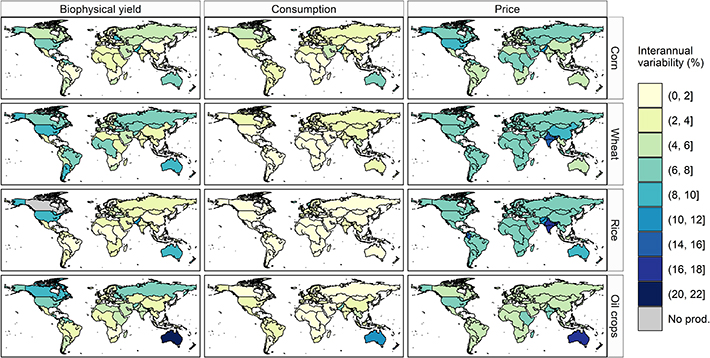
The economic responses to biophysical variability, though generally consistent across climate scenarios at the global scale, were considerably heterogeneous across regions and crops within a scenario. Crop-regions with higher IAV of biophysical yield shocks tended to have a higher IAV in economic responses while the relationship was substantially nonlinear, particularly for consumption and prices (figure 5 and SI figures S11–S13), as also indicated by the high heterogeneity in RIV (figure 4). It was mainly because the IAV of consumption and prices was mediated across crops and regions through crop substitutions and international trade. That is, crop-regions with higher (lower) IAV of biophysical yield shocks tend to have a smaller (larger) magnitude of variance transmission to consumption and price responses, i.e. smaller (larger) RIV. Note that if the magnitude of IAV transmissions from biophysical yield shocks to market responses is the same across crop-regions (e.g. perfect foresight with no trade or other crop-region specific market-mediated responses), RIV should be the same across crop-region. Thus, a negative relationship between RIV and IAV of biophysical yield suggests a mediation effect across crop-regions (SI figure S14). Also, the mediation effects are important regardless of the expectation schemes, while the effects were stronger under adaptive expectation, as implied by the steep slopes compared with perfect foresight. Despite being subject to barriers and costs, trade plays a unique role in reducing agricultural market variability from climate impacts, particularly when consumption is sourced from regions with negatively correlated biophysical yield shocks or crop supply responses. Thus, the IAV distributions of consumption across regions mostly 4 have a smaller dispersion due to the mediation effect, but also shifted to the left, implying a reduction effect (i.e. RIV < 1 for consumption), compared with the IAV distributions of biophysical yield shocks (SI figure S15). However, the reduction effect was not seen for price distributions mainly because of the endogenous market fluctuations (see SI section S3.2 for additional discussions on regional results). This could also be true at the sub-regional level, given the high spatial heterogeneity of climate impacts on crop productivity, that intraregional trade could help reduce and mediate market variability due to climate impacts.
Figure 5. IAV in biophysical yield shocks and the economic responses in the GE scenario. Maps of regional IAV in biophysical yield shocks and the consumption and price responses for major crops (corn, wheat, rice, and oil crops) from the GFDL-ESM2M and EPIC (GE) scenario, estimated under adaptive expectations. Results from other climate scenarios are presented in SI figures S11–S13. Gray areas in biophysical yield maps represent regions with no productions of the crop. Data source: GCAM simulation results.
Download figure:
Standard image High-resolution image
4. Discussion and conclusions
To our knowledge, this is the first study to systematically examine how global agriculture responds to climate and biophysical variability. However, there are some limitations in our analysis. Although we focused on assessing climate impacts from the natural climate-induced biophysical shocks, other external shocks such as extreme weather events and government policies may further buffer or exacerbate the economic responses, depending on the magnitude of the variation and the extent to which agricultural producers predict these shocks. There have been recent efforts on improving the representation of weather variations in climate and crop models (Frieler et al 2017b, Betts et al 2018). With improved biophysical assessments of weather variations and extremes, our model can be used to evaluate their interannual agroeconomic impacts. Also, there could be great uncertainties around endogenous market fluctuations regarding the magnitude of the responses, the heterogeneity of the responses across regions and crops, and the rationality and heterogeneity of the expectation schemes. Our sensitivity tests on the coefficient of expectation in adaptive expectation indicate that with faster adjustment in expectation implied by the higher coefficient of expectation, biophysical shock triggered endogenous market fluctuations would become stronger so that the IAV increases for all economic variables, with relatively higher sensitivity for price and harvested area (see supplementary discussions in SI section S2.2). Future studies are needed to improve expectation schemes and estimated the associated responses with regional and sectoral specifications. Empirical studies demonstrated incorporating expected prices and yield provided better identifications in evaluating agricultural supply responses (Roberts and Schlenker 2013, Hendricks et al 2014, Calvin et al 2017), and it is certain that with no endogenous market fluctuations, results from perfect foresight would exaggerate adaptation responses and underestimate market variations.
Furthermore, it has been challenging to include stockholding in global economic models (Diffenbaugh et al 2012, Urban et al 2012), which would likely have a moderating impact on market volatility (Williams and Wright 2005, Wright 2011). Realistic modeling of storage would also require information on storage cost, government interventions, and stochastic exogenous shocks, which are usually not available at the global scale (Wright and Williams 1982, Williams and Wright 2005). As with many studies, we abstract from including a speculative interannual stockholder and do not investigate the interplay between storage and climate impacts (Diffenbaugh et al 2012, Urban et al 2012). Also, futures and options markets are not considered in our model, which may have additional market implications (Gohin and Zheng 2020). Nevertheless, the main impacts from including storage and other speculative markets implied by a stochastic competitive storage model (Lowry et al 1987, Gouel 2012, Femenia 2015, Schewe et al 2017), e.g. positively skewed and shifted price distribution, could be partly reflected in a deterministic adaptive expectation model by adjusting production cost and coefficient of expectation. In particular, agricultural producers, when improving the accessibility to speculative markets, will likely have a slower adjustment in adaptive expectation, i.e. a smaller coefficient of expectation, and resulting in reduced variability in market responses (see figure S7). Future studies are needed to refine data and parameters to study impacts from storage or other speculative markets under a changing climate.
This paper focused on four widely used climate scenarios of future biophysical yield shocks and showed relatively consistent economic responses to biophysical IAVs (i.e. RIV) at the global scale while highlighting the important role of trade in explaining regional heterogeneity in the responses. It is also important to note that the high uncertainty in biophysical yield projections, particularly at the regional scale, would be mirrored in the IAV of their economic responses (see discussions of regional decompositions in SI section S3.2). More scenarios could be explored using more recent climate and biophysical data (e.g. ISIMIP2b data in Frieler et al (2017a)) in the context of model intercomparison tasks using the framework showcased in this paper. These caveats notwithstanding, our study provides fundamental new insights on climate impacts on agricultural market variability and lays the foundation for further investigating the full range of climate impacts on biophysical and human systems.
Acknowledgments
The authors are grateful for the support from the US Department of Energy, Office of Science, as part of research in the Multi-Sector Dynamics, Earth and Environmental System Modeling Program. The Pacific Northwest National Laboratory is operated for DOE by Battelle Memorial Institute under Contract DE-AC05-76RL01830. We acknowledge Page Kyle, Benjamin Bond-Lamberty, Gokul Iyer, and other GCAM team members for their valuable contributions.
Data availability statement
The data that support the findings of this study are openly available at the following URL/DOI: https://doi.org/10.25412/iop.14939337.v1.
Footnotes
- 1
The annual estimates of biophysical yield provided by climate and crop models have hardly been used in global economic models.
- 2
Note that the estimated 2050 climate impacts would be different if using a different base year. Estimates provided here are average values across models and scenarios, under RCP with end-of-century radiative forcing of 8.5 W m−2.
- 3
A recent study from Ortiz-Bobea et al (2021) estimated a 21% TFP loss due to anthropogenic climate impacts in 1961–2015.
- 4
There could be exceptions since the mediation effects across regions may interact with the effects across crops. That is, crop substitution may dominate trade so that mediation effects across regions were not evident, e.g. corn under HE and HL.