
Abstract
In permafrost soils, 'excess ice', also referred to as ground ice, exists in amounts exceeding soil porosity in forms such as ice lenses and wedges. Here, we incorporate a simple representation of excess ice in the Community Land Model (CLM4.5) to investigate how excess ice affects projected permafrost thaw and associated hydrologic responses. We initialize spatially explicit excess ice obtained from the Circum-Arctic Map of Permafrost and Ground-Ice Conditions. The excess ice in the model acts to slightly reduce projected soil warming by about 0.35 °C by 2100 in a high greenhouse gas emissions scenario. The presence of excess ice slows permafrost thaw at a given location with about a 10 year delay in permafrost thaw at 3 m depth at most high excess ice locations. The soil moisture response to excess ice melt is transient and depends largely on the timing of thaw with wetter/saturated soil moisture conditions persisting slightly longer due to delayed post-thaw drainage. Based on the model projections of excess ice melt, we can estimate spatially explicit gridcell mean surface subsidence with values ranging up to 0.5 m by 2100 depending on the initial excess ice content and the extent of melt.
Export citation and abstract BibTeX RIS

Content from this work may be used under the terms of the Creative Commons Attribution 3.0 licence. Any further distribution of this work must maintain attribution to the author(s) and the title of the work, journal citation and DOI.
1. Introduction
The Arctic region has undergone rising air temperature over the past half-century and has warmed at a rate greater than the rest of the Earth (ACIA 2005, IPCC 2014). In turn, permafrost temperatures have been increasing (Romanovsky et al 2010) and active layer depths have thickened in many regions (Shiklomanov and Nelson 2002). Further, warming in the Arctic may initiate climatic feedbacks (Hinzman et al 2005, McGuire et al 2009). For example, thawing of permafrost may result in land surface subsidence and changes in local hydrology (Jorgenson et al 2006, Smith et al 2005) along with liberation of carbon stocks currently trapped in frozen ground via faster decomposition (Koven et al 2011, Schaefer et al 2011, Schneider von Deimling et al 2012, Schuur et al 2009, Schuur et al 2013). Therefore, understanding the details of potential permafrost thaw trajectories is required to predict the fate of an estimated 1700 Pg of carbon currently stored in soils in the permafrost regions (Schuur et al 2008, Tarnocai et al 2009) and to elucidate the role of the terrestrial Arctic in broader climate feedback cycles (McGuire et al 2009).
Recent advances in the Community Land Model (CLM) have improved the representation of permafrost by accounting for the thermal and hydrologic properties of organic soil, deepening the soil column, explicitly treating active layer hydrology, and including a vertically-resolved carbon cycle model including CH4 emissions (Koven et al 2013b, Lawrence et al 2008, Lawrence and Slater 2008, Riley et al 2011, Swenson et al 2012). CLM modeling studies indicate that large-scale degradation of near surface permafrost may occur by the year 2100, with the degradation exceeding 50% of the current near-surface permafrost under a 'business-as-usual' CO2 emission scenario (RCP8.5; Lawrence and Slater 2005, Lawrence et al 2012b). Other recent modeling efforts (MacDougall et al 2013, Schaefer et al 2011) and analysis of CMIP5 (Coupled Model Intercomparison Project Phase 5) results show strong diversity in the amount and rate of permafrost thaw and suggest that poor representation of several key processes in permafrost may be causing this diversity in these large scale models (Koven et al 2013a, Slater and Lawrence 2013). Developments in land surface schemes can capture small scale differences in altitude (Fiddes et al 2013), terrain, subsurface processes (Langer et al 2013, Zhang et al 2013) including drainage properties and active layer, as well as simplified snowpack and snow redistribution (Dankers et al 2011, Winstral et al 2002) and insulating moss cover (Ekici et al 2014). These efforts enable ground thermal simulations at higher spatial and temporal resolution in complex permafrost landscapes and more sophisticated simulations of permafrost thaw processes. However, most large-scale models do not resolve several potentially important processes that are likely to affect permafrost projections including vegetation interactions, aspect, slope, micro-climate, excessive ground ice, thermokarst, and fire-thaw feedbacks (Grosse et al 2011, Rowland et al 2010). Here, we address one of these limitations by incorporating a simple treatment of excess ice in CLM and assessing its impact on permafrost dynamics under historic and future climate change scenarios.
Excess ice bodies slowly form over long time periods as a result of repetitive contraction and expansion associated with seasonal cycles of subsurface thawing and refreezing. They grow in forms of large ice lenses and ice wedges within the subsurface layers (Davis 2001) and alter soil thermal properties such as the overall thermal conductivity and heat capacity, as well as soil moisture conditions. As a result, excess ice may have a large impact on the rate of permafrost thaw due to the latent heat required to melt the extra ice (Woo 1986). In addition, when ice rich permafrost thaws, the land surface formerly sustained by ice wedges and lenses can collapse and create land surface subsidence. This land surface subsidence, also called thermokarst, alters local hydrology (Jorgenson et al 2006, Osterkamp et al 2009) and can potentially influence the rate and the magnitude of permafrost carbon loss and subsequent greenhouse gas emissions, possibly accelerating future climate change (Lee et al 2011, Lee et al 2012, Schuur et al 2009, Vogel et al 2009, Walter et al 2008).
In this study, we incorporate excess ice within the subsurface soil profile of the CLM to improve the characterization of permafrost landscapes and to set the stage for prognostic wetland dynamics modeling as permafrost thaws. This enables us to address two questions. (1) What impact does excess ice have on the transient response of soil temperature and soil moisture under climate change? (2) Can we model gridcell-specific land surface subsidence under changing climate using a global scale model by incorporating excess ice?
2. Methods
The CLM is the land component of the Community Earth System Model (Lawrence et al 2011). It is a process-based model that includes modules to simulate biogeophysical processes including solar and longwave radiation that interacts with canopy and soil, momentum and turbulent fluxes from canopy and soil, heat transfer in soil and snow, hydrology of canopy, soil, and snow, stomatal physiology and photosynthesis, and carbon and nitrogen (C and N) cycle representing biogeochemical cycles in plants and soil. The thermal and hydrological properties of the soil are determined by a weighted combination of mineral and organic soil content (Lawrence and Slater 2008). Heat conduction through the soil depends on the thermal and hydrological properties of each soil layer and is a function of soil liquid and ice water content, texture (sand, silt, clay, organic), and temperature. A comprehensive technical description of CLM4.5, the version utilized in this study, is provided in Oleson et al (2013). Several changes explicit to cold region hydrological processes were included in CLM4.5, which resulted in significantly improved simulations of active layer and permafrost hydrology and soil temperatures by correcting for the unrealistic conduction of liquid water through frozen soils (Swenson et al 2012).
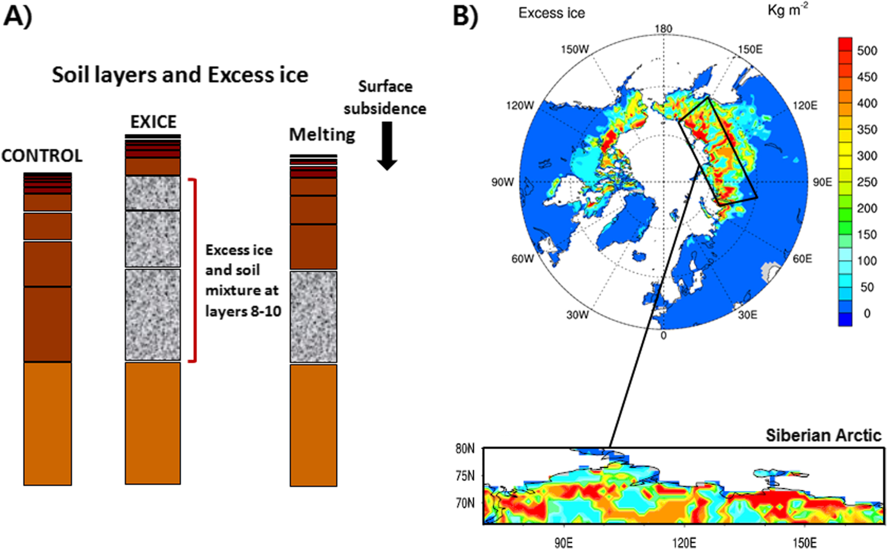
Here, we aim to understand how the presence of excess ice may affect the trajectory of permafrost extent and ground conditions under warming. We do not model the long-term process of excess ice formation; instead, we specify the initial state of a gridcell-specific thickness of ice in the CLM soil layers based on ground ice data from the Circum-Arctic Map of Permafrost and Ground-Ice Conditions (http://nsidc.org/data/ggd318.html; Brown et al 1997). This dataset describes estimates of the distribution of permafrost and properties of ground ice in the Northern Hemisphere (20°N–90°N) and provides a classification of permafrost type and approximate range of percent volume of ground ice at 25 km resolution as continuous, discontinuous, sporadic, or isolated permafrost boundaries that shows permafrost extent estimated in percent area (90–100%, 50–90%, 10–50%, <10%, and no permafrost) and relative abundance of ground ice in the upper 20 m estimated in percent volume (>20%, 10–20%, <10%, and 0%). We re-gridded the original 25 km resolution classifications to the 1-degree default resolution for CLM. Using this information, we generated an estimate of the mean gridcell-specific excess ice volume. The excess ice incorporated in each gridcell is exposed to gridcell-specific climate forcings and demonstrate different timing and magnitude of melting. For the medium excess ice case, the maximum amount of extra ice is 24%, which is equivalent to 74 Kg m−2 of water or approximately 680 mm of excess ice thickness within the soil column.
The CLM has 15 soil layers by default extending to a depth of 48 m; the top 10 soil layers (to a depth of 3.8 m) are hydrologically active with the remaining deeper layers representing bedrock. The excess ice is added into CLM soil depths between 0.8 and 3.8 meters (typically below the active layer) by increasing the thickness of each relevant soil layer and filling the extra soil layer thickness with ice water (see figure 1(A) for schematic illustration). As a result, excess ice is prescribed to be similar to evenly distributed mixture of ice and soil across a single gridcell. As excess ice is incorporated below the active layer in most locations, there is little to no change in excess ice after the spinup. The dataset used to estimate excess ice only contains excess ice where permafrost exists, but the CLM does not have subgrid-scale distribution of permafrost extent. Here, we determined excess ice amount by multiplying the percent permafrost area for each gridcell by the medium excess ice estimate for the total amount of excess ice for each CLM gridcell. We did not attempt to explicitly simulate ice wedge formation and distribution as this would require sub-grid scale resolution and processes, such as crack formation within the soil profile, that are not modeled.

Figure 1. A conceptual diagram of incorporating excess ice in the soil layers of the CLM4.5 (A) and the distribution of ground ice with medium level excess ice incorporation (B). The boxed area represents Siberian Arctic, which we used for closer investigation of changes in soil thermal and moisture properties.
Download figure:
Standard image High-resolution imageBy incorporating excess ice in the soil layers, the standard model soil layer thicknesses are increased to account for the volume of excess ice. The revised soil layer depth at layer i, denoted as z'i (m), is the sum of the original soil layer depth (zi) plus the additional thickness due to excess ice. Including excess ice in this way allows us to simulate soil layer thickness dynamically with the thickness of the soil layers decreasing as excess ice melts. The excess ice affects soil temperature through its influence on heat flux and phase change. Heat flux is a function of soil thermal conductivity and soil heat capacity. Heat flux Fi (W m−2) from layer i to layer i + 1 and thermal conductivity at the interface λ[zi] are computed at each specific soil layer and layer interface to include the impact of the extra volume of ice:
where Ti is soil temperature at the layer node depth z'i. The thermal conductivity λ[z'i] is defined at the interface of two layers z'i and z'i+1.
Several additional modifications are made to incorporate excess ice including modifications to soil heat capacity and total phase change energy. Soil heat capacity at layer i is modified to
where ci is soil heat capacity of a layer (J m−2 K−1) from de Vries (1963); cs is the heat capacity of soil solids (J m−3 K−1), θsat is the volumetric soil water at saturation, Δzi is the soil layer thickness of layer i, Cice,i, Cliq,i, and Cexice,i are the specific heat of soil, ice, and excess ice water at layer i (J kg−1 K−1), and wice and wliq are ice and liquid water content (kg m−2), and wexice is gridcell specific excess ice content (kg m−2) of soil based on Brown et al (1997). The phase change energy equation is rewritten to
where Ep is the total phase change energy (W m−2), Lf is the latent heat of fusion for ice (J kg−1), wice0 is the initial mass of ice (kg m−2), Δt is the change in time, wexice0 is the initial mass of excess ice (kg m−2). It is important to note here that the energy and water is conserved and checked with balance at each time step of 30 min throughout.
During phase change, we require that all soil ice in a layer melts before excess ice is allowed to melt. As excess ice melts, the melt water is added to the soil liquid water of the host soil layer. If the additional water means that the soil layer is above its soil water capacity (as determined by its porosity), any excess water is added to an unsaturated soil layer above it. This water is then subjected to normal CLM soil water movement and runoff generation mechanisms. At the same time, the soil thickness used in the CLM thermal equations dynamically shrinks as excess ice melts. Once excess ice melts, it cannot reform.
A pair of simulations was conducted for the years 1850 to 2100: (1) a case with the standard version of the model ('CONTROL') and (2) a case where excess ice was incorporated within the soil profiles ('EXICE'). For each experiment, we forced the model with identical 3-hourly climate forcing data obtained from a single ensemble member of a historical and projection (RCP8.5) simulation with CCSM4 (Meehl et al 2012). We separately spunup the CONTROL and EXICE versions of the model for 100 years with repeated year 1850 climate and greenhouse gas forcing. Soil temperatures down to the base of CLM (∼42 m) are well equilibrated after the spinup. The CLM model state from the end of the spinup is used to initialize each experiment. The C and N cycle option is turned off for these experiments to avoid complications associated with introducing this extra degree of freedom and to circumvent the long spinup time required. Additional simulations with the excess ice module and active biogeochemistry with CH4 emissions are planned.
The RCP8.5 scenario is a high greenhouse gas emissions scenario (Moss et al 2010). In CCSM4, this scenario results in strong warming in the Artic (Lawrence et al 2012b). We acknowledge that the CCSM4 coupled model climate contains biases in the Arctic, particularly excessive snowfall across much of the region which leads to excessive soil insulation that tends to result in permafrost soil temperatures that are warmer than comparable simulations forced with observed climate. As a result, permafrost thaw occurs more rapidly in CLM when forced by CCSM4 climate than when the climate biases are removed (Lawrence et al 2012a). For the purpose of this study, this issue can be neglected since we are focusing on the differences in soil temperature and soil moisture projections associated with incorporating excess ice rather than on the permafrost projection itself.
3. Results
The initial soil temperature conditions (after the 100-year spinup) for the EXICE simulation show only slight differences, in the mean as well as the seasonal cycle, compared to CONTROL for the analyzed Siberian Arctic (66–80°N, 70–170°E, figure 1(B)). The thickness weighted column average soil temperature was slightly warmer in EXICE simulation by 0.14 °C. Soil temperature in EXICE was warmer in the winter and cooler in the summer compared to CONTROL, implying a smaller amplitude seasonal cycle in EXICE (figure 2). This seasonal structure is consistent with results reported in Subin et al (2013), where the addition of a large volume of water within the soil profile resulted in increased heat capacity and thermal conductivity, effectively dampening the annual temperature cycle (Subin et al 2013). In our subsequent analysis, we normalized the soil temperatures by removing the annual mean initial soil conditions to isolate the role of excess ice on the transient soil temperature response from differences in equilibrium soil conditions.
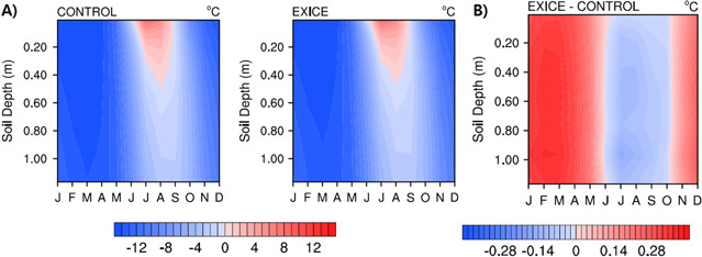
Figure 2. (A) Mean monthly climatology of soil temperature in the Siberian Arctic (66–80°N, 70–170°E) during 1850–1859 after 100-year spinup. (B) Difference in monthly soil temperature between EXICE and CONTROL.
Download figure:
Standard image High-resolution imageIn figure 3(A), we show time series of the difference in soil temperature anomaly between EXICE and CONTROL at 1 and 3 m depth in January and July from 1850 to 2100 (initial conditions removed as noted above) averaged across Siberian Arctic. The EXICE simulation showed slightly less winter soil warming by the year 2100 (∼0.35 °C) with some variability with depth. The summer soil temperature difference was minimal. The difference in cumulative ground heat flux exhibited a sharp increase from the early 21th century (figure 3(B)). The additional ground heat flux in the EXICE is used to melt the excess ice and partially explains why the soil temperature differences are relatively insignificant.

Figure 3. (A) Difference in January and July time series of soil temperatures at 1.0 and 3.0 m depth in the Siberian Arctic (66–80°N, 70–170°E) for EXICE and CONTROL simulations. Soil temperature was corrected from the mean conditions in years 1850–1859 and results shown are 15 year running mean. (B) Difference in cumulative ground heat flux for EXICE and CONTROL simulations and the time series of total excess ice (kg m−2) across the study area.
Download figure:
Standard image High-resolution imageDifferences between EXICE and CONTROL for soil moisture trends were strongly influenced by the timing of active layer thickening and permafrost thaw (figure 4). Figure 4(A) shows the difference in soil moisture trends and the depth of active layer (soil layer where September soil temperature is 0 °C) for two different locations containing relatively high excess ice (24%). At the first location (67°N, 85°E; located in western Siberia), permafrost at this particular location thaws to 3 m depth by the early part of the 21st century, while at the second location (68°N,144°E; located in central Siberia), permafrost thaws much later towards the end of the century. At each site, the active layer thickens with time in response to warming climate (supplementary information 1, available at stacks.iop.org/ERL/9/124006/mmedia). In the EXICE simulation, the presence of excess ice delays active layer thickening and postpones talik formation by approximately a decade (see also in relation to soil moisture, supplementary information 2). In both simulations, soil ice accumulates at the base of the active layer, greatly decreasing drainage below the active layer. This leads to relatively drier conditions below the permafrost table and wetter conditions in the active layer. Because the CONTROL simulation has a thicker active layer, soil moisture values at the bottom of the active layer are higher than those at the same depth in the EXICE simulation, leading to negative soil moisture differences at that depth. When the lowest CLM soil layer thaws, soil water that was impeded by low conductivity icy soils can drain to the model aquifer. When this occurs, positive soil moisture differences were seen between EXICE and CONTROL as the soil column in CONTROL simulation becomes drier than EXICE soil column due to more rapid bottom drainage. At these sites, this condition lasts for roughly ten years before the lowest soil layer in EXICE simulation also thaws. Afterwards, its soil column also dries out, leading to soil moisture conditions converging to those in CONTROL.
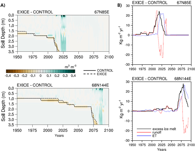
Figure 4. (A) Difference in July soil moisture (volumetric water content, m3 m−3) across depth between EXICE and CONTROL (EXICE—CONTROL) in two different locations within the Siberian Arctic and the depth of active layer for CONTROL and EXICE. (B) A 15-year running mean of excess ice melting, runoff, and evapotranspiration (ET).
Download figure:
Standard image High-resolution imageIn our model setup, melt water from excess ice becomes soil water. As excess ice melts, much of the melt water is converted to runoff (figure 4(B)), leading to higher runoff in EXICE simulation. When the deepest soil layer thaws in CONTROL, the model groundwater component becomes active. This model behavior leads to greater runoff (via baseflow) in CONTROL, which can be seen in the negative runoff differences in figure 4(B). The delay in talik formation due to the presence of excess ice can also be seen in the evapotranspiration (ET) differences, with EXICE continuing to exhibit high evaporative moisture fluxes until its lowest soil layer thaws and the soil column dries out approximately ten years after the same phenomena occurs in CONTROL. The amount of excess ice melting, however, may only have a small impact on river flow as it is still small amount of water in relation to total runoff (supplementary information 3).
4. Discussion and summary
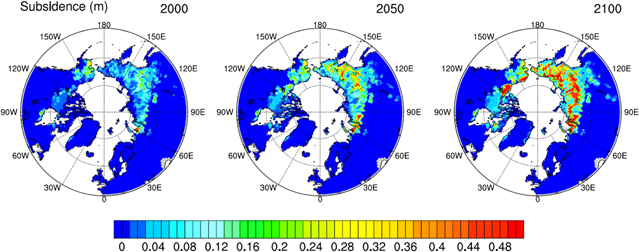
One of the advantages of incorporating excess ice in the model is that excess ice enables a first estimate of large-scale land surface subsidence that results from melting soil and excess ground ice. In our simulations, the amount of excess ice in the Siberian Arctic remained relatively stable until 2050, but mostly disappeared by the end of the 21st century. Note that the climate biases in CCSM4 tended to lead to earlier permafrost thaw than when these are bias corrected with observed climate estimates (Lawrence et al 2012b), so the rate of excess ice melt in this configuration is likely accelerated. Nonetheless, we can estimate patterns of surface subsidence (figure 5). By the end of the 21st century, excess ice melted on average 71% globally, in some locations 100%. These patterns, not surprisingly, reflect those of the initial excess ice distribution. These estimates are in agreement with recent observations in Alaska (Liu et al 2012, Shiklomanov et al 2013) where a decade of land surface subsidence observations showed only tens of centimeters change across the observed landscape.
Figure 5. Gridcell mean land surface subsidence (m) as a result of excess ice melting in year 2000, 2050, and 2100 simulated using climate conditions of historic CESM simulations (1850–2004) and RCP8.5 scenario (2005–2100).
Download figure:
Standard image High-resolution image
Our model setup of excess ice melt, therefore, could be used to infer the timing and magnitude of land surface subsidence and associated thermokarst development, and possibly changes in wetland distributions on a gridcell scale (10–100 km horizontal resolution). The coarse resolution of the model prevents explicit simulations of landscape processes such as runoff generation or thermokarst development across the Arctic landscape that often occur at much smaller scales (a few meters to kilometers), but the development of parameterizations relating gridcell mean subsidence to changes in the statistical distribution of fine-scale topography may help improve the projection of changes in near-surface hydrology in the Arctic. More realistic predictions of changes in land surface processes in permafrost regions will enable better simulations of CO2 and CH4 dynamics in the Arctic landscape under a warmer climate.
In summary, we evaluated the large-scale effects of excessive ground ice on projected permafrost temperature and soil moisture dynamics. Our results demonstrate that excess ice affected the vertical structure of soil temperature and moisture and may influence the rate and timing of permafrost thaw. Our excess ice parameterization remains necessarily simplistic. In order to capture the full impact of excess ice, future model developments may need to emphasize subgrid-scale representation of ground ice distribution within the landscape (e.g., ice wedges). In future work, we intend to explore whether or not it is possible to link excess ice melt and the associated implied surface subsidence with large-scale estimation of changes in wetland distribution and associated CH4 dynamics, which would enable a more comprehensive examination of the possible trajectory of the permafrost carbon-climate feedback cycles under changing climate.
Acknowledgments
We thank Erik Kluzek for technical support. This work was funded by NSF EaSM—L02170157 to AGS, DML, and SCS.