Adaptive Edge Preserving Weighted Mean Filter for Removing Random-Valued Impulse Noise

Abstract

This paper proposes an adaptive noise detector and a new weighted mean filter to remove random-valued impulse noise from the images. Unlike other noise detectors, the proposed detector computes a new and adaptive threshold for each pixel. The detection accuracy is further improved by employing edge identification stage to ensure that the edge pixels are not incorrectly detected as noisy pixels. Thus, preserving the edges avoids faulty detection of noise. In the filtering stage, a new weighted mean filter is designed to filter only those pixels which are identified as noisy in the first stage. Different from other filters, the proposed filter divides the pixels into clusters of noisy and clean pixels and thus takes into only clean pixels to find the replacement of the noisy pixel. Simulation results show that the proposed method outperforms state-of-the-art noise detection methods in suppressing random valued impulse noise.

1. Introduction

For image analysis, de-noising is an important pre-processing step. Digital images are oftentimes corrupted by impulse noise during acquisition, transmission and impaired camera sensors [1], which degrades image features such as edges, sharpness, depth, etc. These degradations can severely hamper the performance of some post-processing steps such as image segmentation, edge detection, feature extraction, target detection, recognition and classification. Therefore, the removal of impulse noise from these images is one of the most fundamental problems in the field of digital image processing. It refers to the removal of noise from corrupted images and the preservation of useful information such as edges and discontinuities. Unlike Gaussian noise, Impulse noise does not corrupt every pixel in the image. It corrupts only certain number of pixels based on noise density. Impulse noise is of two types: Salt & Pepper Noise (SPN) and Random Valued Impulse Noise (RVIN) [2]. SPN corrupts image with two fixed extreme Values while RVIN takes any arbitrary value in range [$n_{min}$, $n_{max}]$. For 8-bit images, $n_{min}$ = 0 and $n_{max}$ = 255. Therefore, detection of RVIN is much more complex and difficult as compare to SPN [3]. For simplicity, let $x_{i,j}$ and $c_{i,j}$ be the intensities of pixels of noisy and original images, respectively. Then, the noise model for RVIN [4] can be described as:

$$\begin{array}{c}\hfill x_{i,j}=\left\{\begin{array}{cc}{c}_{i,j},\hfill & \mathrm{for}p=1-p_0,\hfill \\ n_{i,j},\hfill & \mathrm{for}p=p_0,\hfill \end{array}\right.\end{array}$$

(1)

where $n_{i,j}$ shows gray level of uniformly distributed noise in range [$n_{min}$,$n_{max}$] while $p_0$ is the probability of noise.

To suppress impulse noise, different filters have been used. However, most of these filters have a disadvantage of losing some important information such as edges [5]. These are simple low pass filters where, for every pixel, some operation is performed on all the neighboring pixels in the predefined window and the result replaces the central pixel. The simplest filter to remove impulse noise is median filter (MF) [6]. This filter replaces every pixel in the image by the median value of the given window, irrespective of whether the pixel is noisy or non-noisy. Though MF is computationally simple and less expensive, but as the clean pixels are also replaced by median value of the selected window, this degrades the quality of image, and also produces edge jitters and streaking. Similarly, some patches are also created at higher noise density [7].

To make a trade-off between edges preservation and complexity, multiple variants of MF [8] have been proposed. Some proposed variants are Tri-State Median filter (TSMF) [9], Recursive Weighted Median Filter (RWMF) [10], the Multi-state Median Filter [11] the Central Weighted Median Filter (CWMF) [12], the Rank-Order Mean Filter and the Stack Filter [13]. However, these filters still degrade the quality of images as they replace all pixels in the image without considering whether the test pixel is noisy or not [14]. To overcome this drawback, several filtering schemes have been developed which are integrated with noise detectors. In these techniques, image de-noising is performed in two stages. In the first stage, the noisy pixels are detected by approximation from neighborhood pixels. In the second stage, only those pixels which are detected as noisy are cleaned while remaining pixels are left unchanged. The performance of detection stage heavily depends on the estimation of proper threshold value. A prior threshold is used by most of the techniques, where the predefined threshold is used throughout the image. Some notable examples of the filtering techniques which use a fixed threshold for noise detection are: adaptive center-weighted median (ACWM) filter [15], the optimal direction median filter [2], the two-pass switching rank-ordered arithmetic mean (TSRAM) [16] filter, Progressive Switching Median Filter (PSMF) [17], Luo-Iterative Median Filter (Luo) [18], Directional Weighted Median (DWM) filter [19], the contrast Enhancement-based Filter (CEF) [20] and robust outlyingness ratio non-local mean (ROR-NLM) [21], etc. The ACWM supresses the RVIN by using the difference between the output of CWM and the current pixel. In CEF, exponential function is used to enlarge the differences, which are then summed to detect the noisy pixels. The DWM only considers pixels along four certain directions to detect noise. Once the noise is detected, the noisy pixel is replaced by weighted median value in the optimal direction. In ROR-NLM [21], the weights of non-local means filter (NLM) [22] were used as noise detectors on initial denoised image. These filters usually perform well at lower noise density. However, at higher noise density, these filters have limited performance in terms of image details and edges preservation. This is because the statistics of the image are not uniform for the whole image, so the threshold value suitable for specific region may not be adapted well to other region in same image. In addition, the threshold value adjusted for a particular image may not work well for other image.

In order to reduce the shortcomings of the fixed threshold scheme, an Adaptive Switching Median Filter (ASWM) [23] was proposed. This filter automatically defines a new threshold for every pixel based on the local standard deviation, and does not require a priori knowledge for the threshold selection. Though this filter provides better detection results, when the noise is not too much high. However, due to random noise, some intensity values of noisy pixels may be very different from other neighbor pixels inside a current sliding window—in which case, the standard deviation of current window is very large, which can result a very large threshold. Thus, the higher standard deviation can cause inaccurate calculation of the local threshold. Secondly, the detected noisy pixel is replaced with simple median value of the whole current window. As the current sliding window also contains noisy pixels, the median value of such noisy window is thus not always accurate. This leads to incorrect replacement of a noisy pixel. Thus, the image details are not preserved. In order to overcome the shortcomings of this technique, we propose an adaptive two staged technique, where, for each pixel processing, a more accurate threshold is calculated. Hence, the main contributions of our proposed technique are:

• We propose an adaptive noise detector and a new weighted mean filter to remove random valued impulse noise from the images.
• In contrast to other state-of-the-art noise detectors, the proposed detector computes a novel adaptive threshold for each pixel. The accuracy of the detection scheme is further enhanced by employing additional steps to avoid faulty detection of edge pixels, which are noisy pixels. This step indeed ensures the preservation of the edges avoiding faulty detection of noise.
• In the filtering stage, a novel weighted mean filter is designed to filter only those pixels which are identified as noisy in the detection stage. In contrast to the existing filtering techniques, the proposed filter first divides the pixels into clusters of clean and noisy pixels. Then, to design the filter, only clean pixels are utilized to find the replacement of the noisy pixel.

Extensive simulation results are presented that show that the proposed RVIN suppression mechanism is superior compared to the state-of-the-art schemes.

2. Proposed Noise Detection Scheme

In this section, we present the proposed efficient noise detector for the detection of noisy pixels. Before the detection process, window size is adjusted for the whole image. The window size is selected adaptively as it is set automatically based on the noise density. To estimate the noise density, we adopt the idea of the universal threshold [24]. In this method, wavelet transform is used to estimate the noise density $\sigma$ of the noisy signal using Robust Median Estimator as:

$$\sigma =\frac{\mathrm{median}(HF)}{0.6745},$$

(2)

where $HF$ is the high frequency sub-band. In this technique, the noisy image or signal is divided into sub-bands of low and high frequencies. The edges, sharp details and sudden changes are found in the high frequencies [25]. Thus, mostly, the high frequency components contain noise. Therefore, only a high frequency sub-band $(HF)$ is used to estimate the noise of the signal, as illustrated in Equation (2). For example, if $\sigma$ comes to be 50, the image has 50% noise and so on. The size of the window depends on $\sigma$, such that, for low $\sigma$, a smaller window is selected, while a larger window is selected for high $\sigma$.

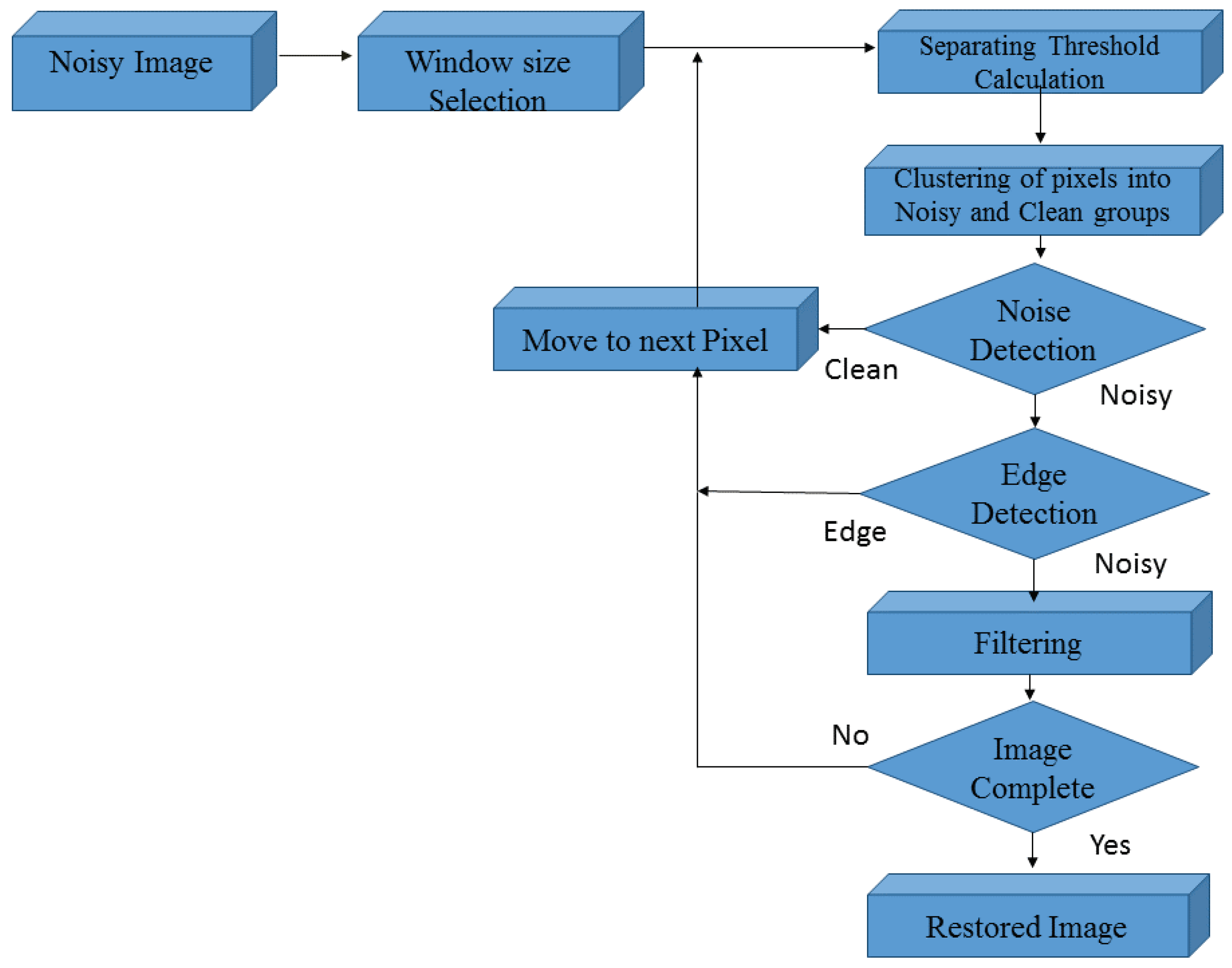
Once the window is adjusted, then the detection process starts. Figure 1 illustrates the block diagram of the proposed noise detector. Each block given in Figure 1 is then elaborated with example in the following subsections.

2.1. Calculation of Separating Threshold

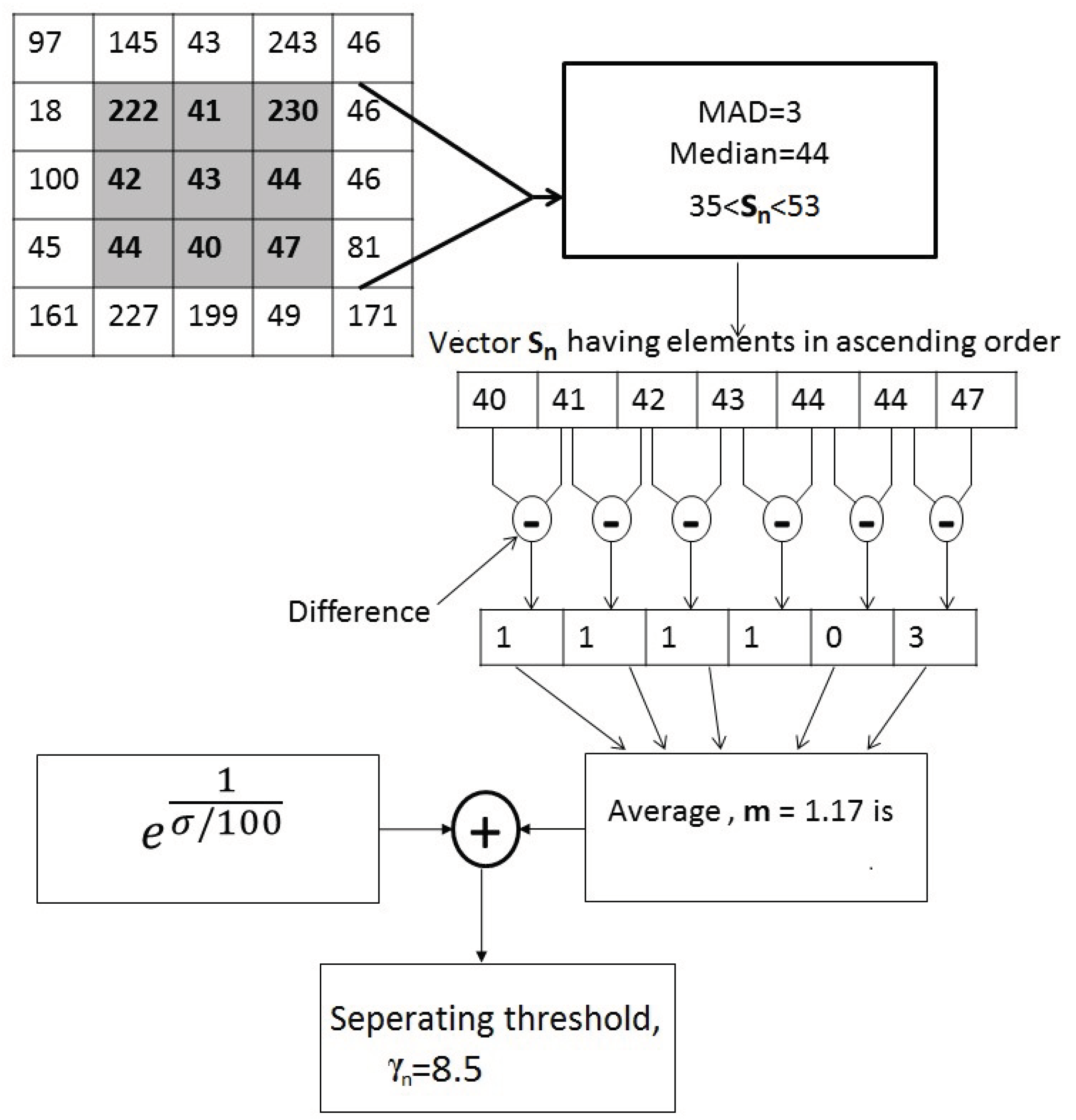
Once the window size is defined, the first step of the proposed noise detection process is the selection of separating threshold ${\gamma }_s$. The algorithm to find separating threshold is illustrated with the help of example in Figure 2 and elaborated in the following steps.

• Let $x_{i,j}$ be the pixel under observation at location $(i,j)$ to know whether it is noise or clean, then it is considered as a central pixel. Window of the size found in Equation (2) is set around the central pixel.
• The corresponding pixel values of of the current window are sorted in ascending order in vector $\mathbf{s}$. The outliers are removed from $\mathbf{s}$ by adopting the “three sigma rule” with median absolute deviation (MAD) [21]. The MAD for $\mathbf{s}$ is found as:

  $$\mathrm{MAD}=\mathrm{median}\mid \mathbf{s}-\mathrm{median}(\mathbf{s}).\mid$$

  (3)
  Vector $\mathbf{s}$ is searched, and, if the difference between any value in $\mathbf{s}$ and the median value is greater than $3\times \mathrm{MAD}$, it is considered as an outlier and is not taken into account for further calculation. After removal of outliers, let ${\mathbf{s}}_{\mathbf{n}}$ be the resultant vector, where n denotes the size of ${\mathbf{s}}_{\mathbf{n}}$.
• Compute the absolute difference $d_k$ between every two adjacent pixels in ${\mathbf{s}}_{\mathbf{n}}$ as:

  $$d_k=\mid s_k-s_{k+1}\mid ,$$

  (4)

  where $k=1,2,\dots ,n-1$.
• The separating threshold ${\gamma }_s$ is found as:

  $${\gamma }_s=m+e^{\frac{1}{\sigma /100}},$$

  (5)

  where

  $$m=\frac{1}{n-1}\sum _{k=1}^{n-1}d(k).$$

  (6)

We can observe that the term $e^{\frac{1}{\sigma /100}}$ depends upon the noise density $\sigma$. It can be observed that, for lower noise density, this term is large and, for higher noise density, this term is small. This term adjusts the threshold to ensure that clean pixels are not considered noisy pixels at very low noise density. Similarly, it also adjusts the threshold to make sure noisy pixels are not grouped into clean pixels, as this threshold will be used in grouping discussed in the following subsection.

2.2. Separation of Pixels into Clusters

Using the separating threshold ${\gamma }_s$, in this section, we divide the pixels in the sorted vector ${\mathbf{s}}_{\mathbf{n}}$ in groups as follows:

• Initialize from the first pixel in sorted vector ${\mathbf{s}}_{\mathbf{n}}$. If the difference between current pixel $s_i$ and next pixel $s_{i+1}$ is less than or equal to ${\gamma }_s$, keep the pixel $s_{i+1}$ in the current group together with $s_i$.
• However, if the difference is greater than ${\gamma }_s$, finish the current group and start a new group, such that the first element of the new group will be $s_{i+1}$. Apply the same procedure until the last element of vector ${\mathbf{s}}_{\mathbf{n}}$.
• The clean and noisy groups are decided based on the size of the group. The first two largest clusters are considered as clean clusters while all other clusters are considered as noisy and are discarded. The clean clusters are denoted as ${\mathbf{g}}_{\mathbf{1}}$ and ${\mathbf{g}}_{\mathbf{2}}$. Cluster ${\mathbf{g}}_{\mathbf{1}}$ is used in the detection phase while ${\mathbf{g}}_{\mathbf{1}}$ and ${\mathbf{g}}_{\mathbf{2}}$ are used in filtering.

2.3. Noise Detection

Using the results of the group stage, in this section, the noise detection stage is presented. The noise detector is:

$$\begin{array}{c}\hfill x_{i,j}=\left\{\begin{array}{cc}\mathrm{Clean},\hfill & \mathrm{if}\mid x_{i,j}-\mu \mid \le \gamma ,\hfill \\ \mathrm{Noisy},\hfill & \mathrm{Otherwise},\hfill \end{array}\right.\end{array}$$

(7)

where threshold $\gamma$ is

$$\gamma =3\times \mathrm{MAD}({\mathbf{g}}_{\mathbf{1}}),$$

(8)

and ${\mathbf{g}}_{\mathbf{1}}$ is the largest group discussed in the grouping stage.

Similarly, $x_{i,j}$ is the central pixel and $\mu$ is the mean value of ${\mathbf{g}}_{\mathbf{1}}$. If the $x_{i,j}$ is detected as noisy, filtering is required to replace the $x_{i,j}$ with the filtered output. On the other hand, if $x_{i,j}$ is a clean pixel, it is left unchanged.

2.4. Edge Pixel Identification

In this section, we present a mechanism to avoid the faulty detection of edge pixels as noisy pixels. This step is performed only when the pixel is identified as a noisy pixel. This will make the detection scheme more robust by verification of the noisy pixels to avoid situations where the edge pixel is wrongly considered as a noisy pixel. This process is performed as follows:

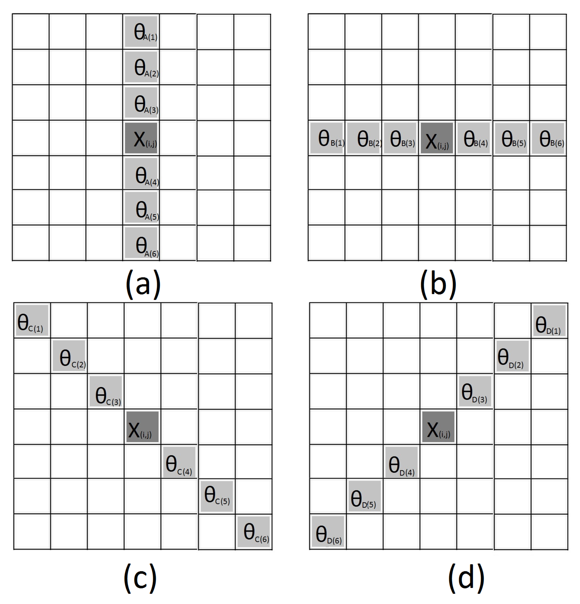
• Keeping $x_{i,j}$ as a reference pixel, pixels present along four directions are taken into account. These four directions ${\mathit{\theta }}_A$, ${\mathit{\theta }}_B$, ${\mathit{\theta }}_C$ and ${\mathit{\theta }}_D$ are illustrated in Figure 3.
• ${\mathit{\theta }}_A^{\prime }$ contains the pixels from the direction ${\mathit{\theta }}_A$ excluding $x_{i,j}$. Similarly, ${\mathit{\theta }}_B^{\prime }$, ${\mathit{\theta }}_C^{\prime }$ and ${\mathit{\theta }}_D^{\prime }$ contain the pixels from the directions ${\mathit{\theta }}_B$, ${\mathit{\theta }}_C$ and ${\mathit{\theta }}_D$, respectively, excluding $x_{i,j}$.
• Find the absolute difference between central pixel $x_{i,j}$ with all pixels along direction ${\mathit{\theta }}_A^{\prime }$. The difference vector is defined as ${\mathbf{d}}^{\mathbf{A}}$ = $\mid x_{i,j}-{\mathit{\theta }}_A^{\prime }\mid$.
• ${\mathbf{d}}^{\mathbf{A}}$ is searched to find the values less than or equal to m. Indexes of pixels corresponding to these values are identified in ${\mathit{\theta }}_A$. These pixels are stacked in vector $\mathbf{v}$. The vector $\mathbf{v}$ is considered to be an edge if total number of pixels in $\mathbf{v}$ is at least 50% of direction ${\mathit{\theta }}_A$. Step 4 is only performed if this condition holds true. Otherwise, discard the $\mathbf{v}$ and go to step 5.
• Take the standard deviation of central pixel $x_{i,j}$ with $\mathbf{v}$. The pixel is identified as an edge if standard deviation of $\mathbf{e}$ and $x_{i,j}$ is less than or equal to threshold $\gamma$:

  $$\begin{array}{c}\hfill x_{i,j}=\left\{\begin{array}{cc}\mathrm{Edge},\hfill & \mathrm{if}\mathrm{std}(\mathbf{v},x_{i,j})\le \gamma ,\hfill \\ \mathrm{Go}\mathrm{to}\mathrm{next}\mathrm{Direction},\hfill & \mathrm{Otherwise}.\hfill \end{array}\right.\end{array}$$

  (9)
• If $x_{i,j}$ is not identified an edge in direction ${\mathit{\theta }}_A$, then the three other directions ${\mathit{\theta }}_B$, ${\mathit{\theta }}_C$ and ${\mathit{\theta }}_D$ are checked for an edge identification by applying the five steps above on each direction.

If $x_{i,j}$ is not identified an edge in all four directions, it is considered a noisy pixel and filtering is required to de-noise it.

3. Illustration

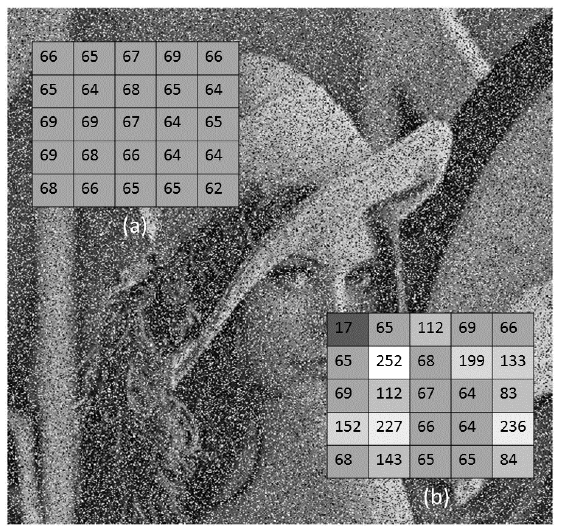
This section illustrates the noise detection of the proposed method with example. Consider the image patch given in Figure 4 that is taken from a 40% noisy “lena” image. The size of the window depends on the noisy density $\sigma$ such that:

$$\begin{array}{c}\hfill \mathrm{Size}\mathrm{of}\mathrm{window}=\left\{\begin{array}{cc}7\times 7,\hfill & \mathrm{if}\sigma \ge 60,\hfill \\ 5\times 5,\hfill & \mathrm{otherwise}.\hfill \end{array}\right.\end{array}$$

(10)

To check whether the specified central pixel is noisy, the following steps are performed.

• Using Equation (2), the noise density of the whole image is calculated. As the noisy density is 40%, therefore, according to Equation (10), the window size is selected 5 × 5.
• Sort all the pixels inside the selected patch in ascending order as $\mathbf{x}$ = [17 64 64 65 65 65 65 66 66 67 68 68 69 69 83 84 112 112 133 143 152 199 227 236 252].
• The extreme outliers are removed by using MAD given in Equation (3). The MAD value of vector $\mathbf{x}$ is 5, while the median value of $\mathbf{x}$ is 69. Therefore, according to the “Three Sigma Rule”, any value below 54 (69 − 15) and above 84 (69 + 15) is discarded and the vector $\mathbf{x}$ becomes [64 64 65 65 65 65 66 66 67 68 68 69 69 83 84].
• Next, the deference between every two consecutive pixels is found to be $\mathbf{d}$ = [0 0 0 0 1 0 1 1 0 1 0 14 2].
• The average value m of the vector $\mathbf{d}$ is equal to 1.4. Putting this value of m in Equation (5), ${\gamma }_s$ becomes 13.59.
• Using the separating threshold, all pixels of $\mathbf{x}$ are divided into groups as [64 64 65 65 65 65 66 66 67 68 68 69 69], [83 84].
• The largest group is [64 64 65 65 65 65 66 66 67 68 68 69 69], whose size is much greater compared to other group. Thus, this group is considered the clean group, while the other group is considered the noisy group.
• Using Equation (8), threshold $\gamma$ becomes 3. Similarly, mean value becomes $\mu$ = 66.
• By employing Equation(9), any value greater than 69 and less than 63 is considered to be noisy.

In this example, the value of the central pixel is 67; therefore, it is a clean pixel and does not need filtering. In case the pixel comes out to the noisy pixel, then we need filtering to replace the noisy pixel with estimated clean pixel. In the next section, we present the filtering scheme.

4. Proposed Filtering Scheme

After the detection of the noise, the appropriate filter is required to replace the noisy pixel. For this, we design a novel Weighted Mean Filter (WMF), which is more robust compared to the existing median and mean filters. In a smooth region, the absolute difference among all neighbor pixels is very small and the whole region is flat [26], so, in most cases, only one large clean group is formed. On the other hand, the region that contains the edge is not as flat, in which case more than one cluster is required to replace the noisy pixel. Therefore, in the proposed filtering scheme, the second largest group ${\mathbf{g}}_{\mathbf{2}}$ is also considered. We remark that the ${\mathbf{g}}_{\mathbf{2}}$ is not required in detection stage. Instead, there is a separate section for edge detection. The two largest groups are assigned weights based on standard deviation and size of the group. Supposing that $x_{i,j}$ is the noisy pixel at location $(i,j)$, then the filtered pixel ${\widehat{x}}_{i,j}$ is given as:

$${\widehat{x}}_{i,j}=\mathrm{mean}\{w_1\diamond {\mathbf{g}}_1,w_2\diamond {\mathbf{g}}_2\},$$

(11)

where ⋄ is the replication operator [27] that shows the repetition of any term. For example, if $w_1$ is 2, and $w_2$ is 1, then ${\mathbf{g}}_{\mathbf{1}}$ is repeated two times while ${\mathbf{g}}_{\mathbf{2}}$ is repeated 1 time, such as ${\widehat{x}}_{i,j}=\mathrm{mean}\{{\mathbf{g}}_{\mathbf{1}},{\mathbf{g}}_{\mathbf{1}},{\mathbf{g}}_{\mathbf{2}}\}$, as the size of ${\mathbf{g}}_{\mathbf{1}}$ is greater than ${\mathbf{g}}_{\mathbf{2}}$. Therefore, to decide the weights, we also consider the standard deviation of both groups. The weights $w_1$ and $w_2$ are determined by a ratio R as:

$$R=\frac{s_2}{s_1}\times \frac{{\mathrm{sd}}_1}{{\mathrm{sd}}_2},$$

(12)

where $s_1$, $s_2$ represents the size, while ${\mathrm{sd}}_1$ and ${\mathrm{sd}}_2$ represent the standard deviation of ${\mathbf{g}}_{\mathbf{1}}$ and ${\mathbf{g}}_{\mathbf{2}}$, respectively. This relation defines the weights of ${\mathbf{g}}_{\mathbf{2}}$ with respect to ${\mathbf{g}}_{\mathbf{1}}$. As the higher standard deviation means less correlation, it is inversely proportional to the R, while the larger size shows larger priority; therefore, it is in direct relation to R. Based on the value of R, the following weights are assigned in Equation (11).

• If the size of ${\mathbf{g}}_{\mathbf{1}}$ is very large compared to the size of ${\mathbf{g}}_{\mathbf{2}}$ or R ≤ 0.5, then $w_1$ = 1, $w_2$ = 0.
• Similarly, when 0.5 $\le R\le$ 1, the assigned weights are: $w_1$ = 1, $w_2$ = 1.
• Finally, for 1 $\le R\le$ 2, the assigned weights are: $w_1$ = 1, $w_2$ = 2.

The filtering is further improved by only considering the closest neighbor pixels of the central pixel from the selected groups, such that, if there are at least three pixels from the selected groups which are in a 3 × 3 window around the central pixel, then take the mean value of only these closest pixels.

5. Summary of the Proposed Denoising Scheme

Although the proposed scheme gives good results in single iterations, with second iterations, it gives the best performance and there is no need to apply further iterations as in other iterative methods. The larger threshold value is used in the first iteration while a smaller threshold value is used in the second iteration [2]. Therefore, if the threshold in the first iteration is 3 × $MAD$, in the second iteration, the threshold is set to 1.5 × $MAD$. We summarize our proposed technique in Algorithm 1 as:

Algorithm 1: Proposed algorithm for random valued impulse noise removal.

Input: The noisy image X, with size of $L_1\times L_2$ 1 Set iteration i = 1. 2 Outer loop: for $l_1=1,\dots L_1$, Inner loop: for $l_2=1,\dots L_2$ 3 Set a sliding window centered at $x_{i,j}$, the size of window is determined by $\sigma$. 4 Divide the window into groups of clean and noisy pixels using separating threshold computed in Equation (5). 5 Find mean $\mu$ and threshold $\gamma$ from clean cluster, while discard the noisy clusters. 6 Using Equation (7) check $x_{i,j}$ for noise. If $\mid x_{i,j}-\mu \mid \le \gamma$, go to step (2). 7 If the pixel is identified as noisy, check $x_{i,j}$ for an edge using Equation (9). Such that if $\mathrm{std}(\mathbf{e},x_{i,j})\le \gamma$, go to step (2). 8 Filter $x_{i,j}$ as in Equation (11). 9 i = i + 1, if $i>i_{max}$, stop iteration, else X ⟵ Y, go to next iteration.  Output: De-noised image Y

6. Experimental Results

To assess the capability the proposed noise removal procedure, in this section, comprehensive numerical results are compared with other state-of-the-art techniques.

6.1. Comparison of Noise Detection

We compare our proposed noise detection scheme with different state-of-the-art techniques such as (ACWM) [15], the (DWM) [19], (TSM) [9] (PSMF [17], (Luo) [18], (ROR-NLM) [21], SBF [28] and (ASWM) [23].

In

Table 1. Detection comparison of different filters at different noise densities.

Methods		40%			50%			60%
	FN	FP	Total	FN	FP	Total	FN	FP	Total
ACWM	14,590	2367	16,857	21,897	3706	25,603	30,198	6526	36,724
Luo’s	14,679	1831	16,510	21,665	3068	24,733	33,987	2780	36,767
TSM	18,921	5201	24,122	23,921	6218	30,139	28,123	8903	37,026
PSM	18,672	4982	23,654	23,762	6123	29,885	27,987	8393	36,380
ASWM	7489	11,564	19,053	11,779	12,786	24,565	19,982	16,482	36,464
DWM	11,786	8931	20,717	15,321	8756	24,077	15,728	14,816	30,544
SD-OOD	13,500	10,675	24,175	11,987	15,827	27,814	17,821	18,261	36,082
ROR-NLM	12,890	3328	16,218	15,297	3487	18,784	21,827	7808	29,635
Propoposed	10,908	7973	18,881	11,668	9613	21,241	13,571	9760	23,331

, the noise detection results of noisy “lena” image with noise densities 40%, 50% and 60% are given. The table lists three results of the noise detection: the number of undetected noisy pixels (False Negative), the number of clean pixels that are falsely detected as noisy (False Positive) and the Total number (False Negative + False Positive).

From Table 1, it is clear that the proposed detection scheme has generated less ‘Total’ number than all of the above techniques especially at higher noise density. At lower noise density, only ROR-NLM produces a lower total number, but they produce much higher false negative terms, indicating that they miss most of the noisy pixels, and most of noise patches are left unchanged. Thus, the proposed detection technique shows superiority over other detection schemes. It is because a noise detector is considered to be efficient and robust, if it reduces both false positive and false negative numbers. When the noise density increases, the superiority of the proposed method is clear as it generates far less ‘Total’ terms than all other methods. This means that our technique is more efficient and robust, even at high noise density.

6.2. Comparison of Image Restoration

The de-noising performance of the proposed method is tested on different standard images such as Lena, pepper, Bridge, and Boat with different noise densities. All these images are 8-bit gray scale and have the same size of 512 × 512 pixels. It should be noted that the size of the window is defined only once based on the noise density using Equation (2), which is used on all pixels of the current image. In our case, for noise density less than 60%, window size of 5 × 5 is used, while window size of 7 × 7 is used otherwise. Peak Signal to Noise Ratio (PSNR) is used as quantitative measurement to compare the proposed method with different well known techniques. The PSNR is defined as:

$$\mathrm{PSNR}(\mathrm{dB})=10{\log }_{10}\left(\frac{{255}^2}{\mathrm{MSE}}\right),$$

(13)

where MSE is mean squared error and is defined as:

$$\mathrm{MSE}=\frac{1}{MN}\sum _{i=1}^m\sum _{j=1}^n{\left(O_{i,j}-R_{i,j}\right)}^{{}^2},$$

(14)

where O is the original clean image while R is the output restored image.

Table 2. Peak Signal-to-Noise Ratio (dB) values of different filters for Lena and Pepper image corrupted by random valued impulse noise of different noise densities.

Methods	Lena			Pepper
(Noise Density)	40%	50%	60%	40%	50%	60%
TSM	24.91	22.22	18.98	24.02	22.56	17.78
ACWM	28.12	24.64	20.32	28.12	26.09	21.52
LOU’S	29.62	25.82	22.69	28.41	26.33	23.89
PSM	29.12	25.31	24.23	28.23	25.41	23.83
ASWM	30.91	28.42	26.25	29.02	27.12	25.33
DWM	30.92	28.91	26.51	29.13	27.79	25.48
SBF	30.12	27.12	23.13	28.89	27.02	24.67
ROR-NLM	31.42	29.21	25.61	29.61	27.89	25.45
PROPOSED	31.77	30.01	28.03	29.75	28.11	26.62

and

Table 3. Peak Signal -to- Noise Ratio (dB) values of different filters for Bridge and Boat image corrupted by random valued impulse noise of different noise densities.

Methods	Bridge			Boat
(Noise Density)	40%	50%	60%	40%	50%	60%
TSM	21.55	19.72	17.26	22.89	20.72	17.55
ACWM	23.72	22.19	19.12	25.32	23.56	21.45
LOU’S	23.84	22.78	19.17	25.45	23.78	21.61
PSM	23.65	21.91	19.39	24.98	22.98	20.87
ASWM	24.02	22.69	21.12	26.76	25.26	23.23
DWM	24.07	22.72	21.19	26.83	25.31	23.57
SBF	22.12	21.31	20.15	25.33	24.88	22.67
ROR-NLM	24.27	22.91	21.21	27.23	25.43	24.21
PROPOSED	24.35	23.08	21.75	27.85	26.61	24.87

illustrate comparison of the proposed method with other state-of-the-art methods.

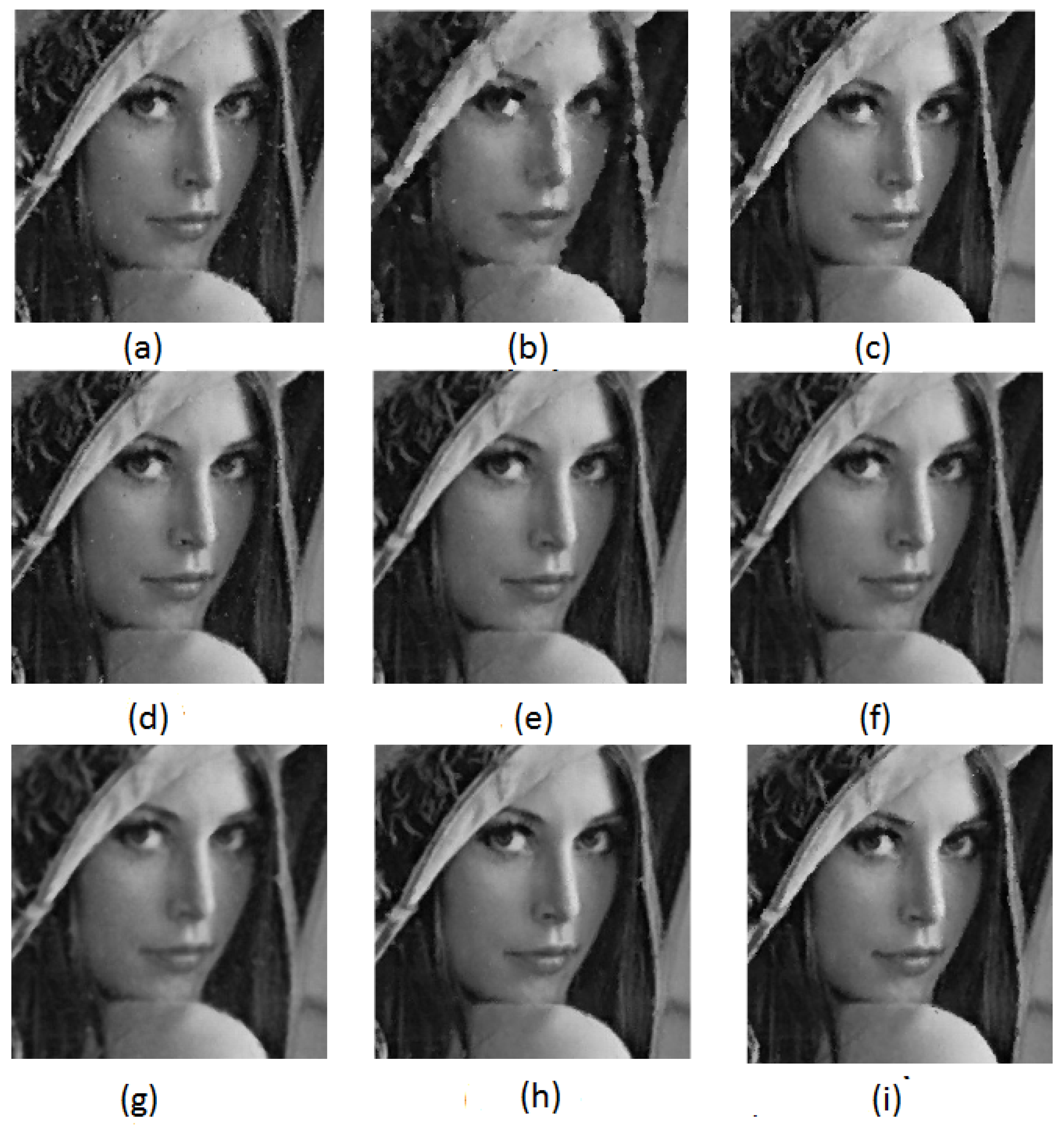
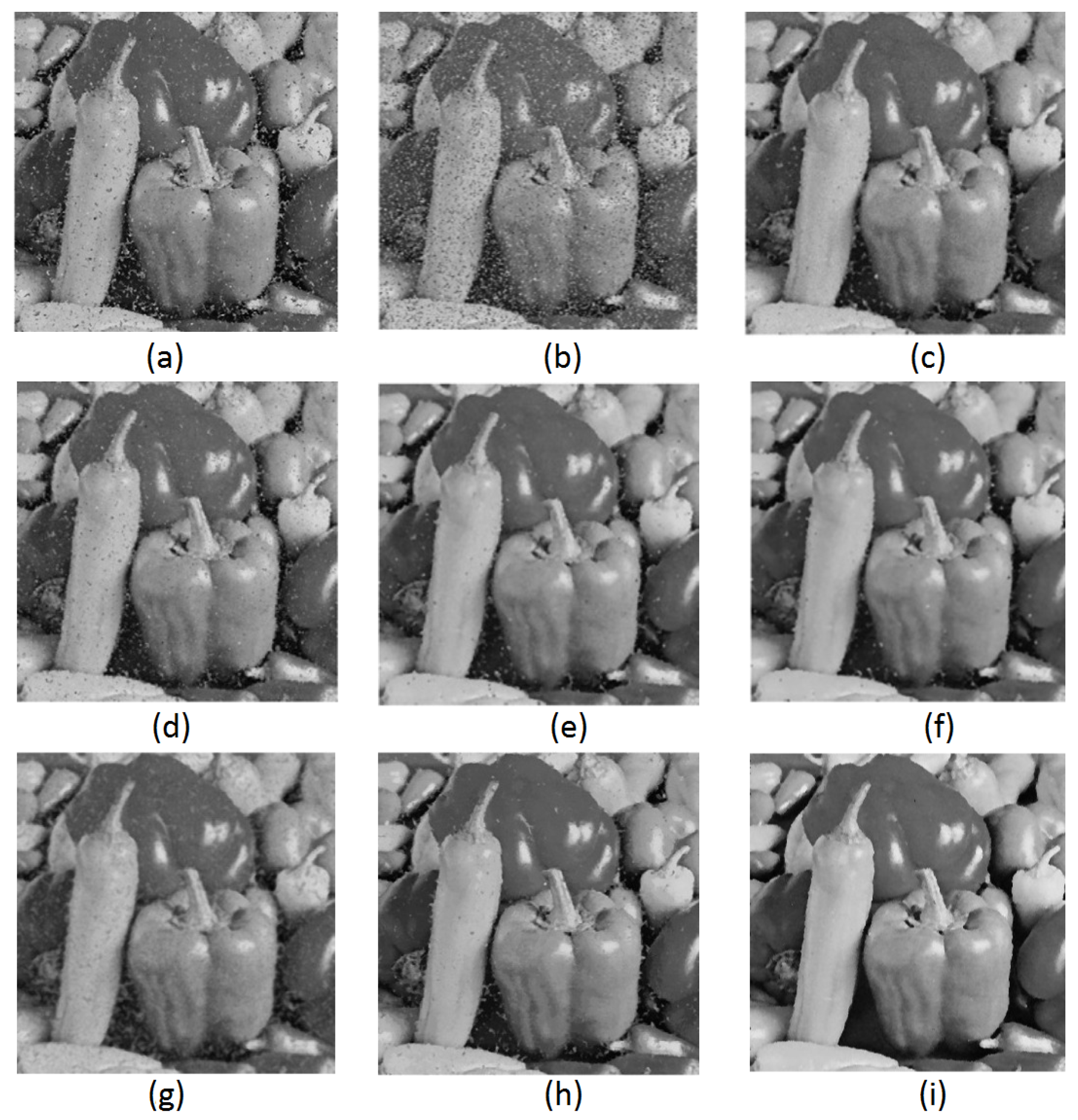
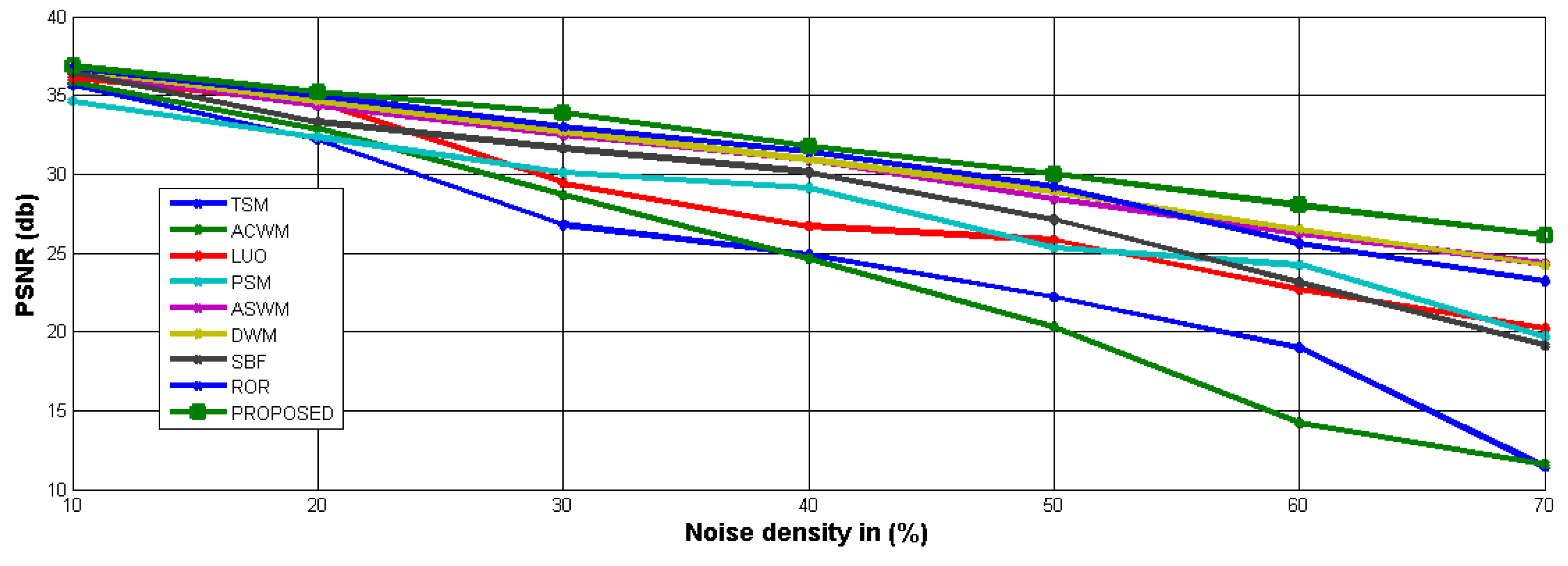
Table 2 and Table 3 list the PSNR values of different test images that are contaminated by RVIN of noise densities ranges from 40% to 60%. From both tables, it is clear that our method has performed better as compared to all other listed methods in terms of PSNR. Figure 5 and Figure 6 show de-noised results of Lena and Pepper images, respectively. From these figures, it is obvious that TSM, ACWM, PSM and Luo have created artifacts and damaged image details. While DWM, ASWM and ROR-NLM have performed better at lower noise densities, but their performance is degraded at higher noise densities. This is due to the fact that these filters replace the noisy pixel by considering all the window pixels. On the other hand, the proposed method only considers clean pixels to replace the noisy pixel. As the noise density increases, the number of corrupted pixels in the window are also increased, which increases the error when the central noisy pixel is replaced by mean or median value of noisy neighbor pixels. Finally, in Figure 7, we present performance results of different filters in restoring Lena image corrupted by different noise densities. These results confirm the results given in Table 2 and Table 3 and clearly show that the proposed method outperforms other state of the art techniques.

7. Conclusions

In this paper, a new algorithm is presented to remove random valued impulse noise. The proposed approach is based on calculation of new and adaptive thresholds for every pixel. The pixels are divided into noisy and clean clusters. Then, only a clean cluster is used to calculate the threshold. A new edge identification step is proposed to ensure that a clean pixel is not considered as a noisy pixel falsely. If the pixel is identified as noisy, a novel weighted mean filter is designed to filter the noisy pixel. Instead of taking the mean of all pixels in the selected window, the proposed filter considers only clean pixels to replace the noisy pixel. Simulation results show that the proposed method outperforms state-of-the-art de-noising techniques, both visually and quantitatively (PSNR), even when the noise density is high.

References

- Gao, G.; Liu, Y.; Labate, D. A two-stage shearlet-based approach for the removal of random-valued impulse noise in images. J. Vis. Commun. Image Represent. 2015, 32, 83–94. [Google Scholar] [CrossRef]
- Awad, A.S. Standard deviation for obtaining the optimal direction in the removal of impulse noise. IEEE Signal Process. Lett. 2011, 18, 407–410. [Google Scholar] [CrossRef]
- Ilke, T. A new method to remove random-valued impulse noise in images. AEU-Int. J. Electron. Commun. 2013, 67, 771–779. [Google Scholar]
- Chan, R.H.; Hu, C.; Nikolova, M. An iterative procedure for removing random-valued impulse noise. IEEE Signal Process. Lett. 2004, 11, 921–924. [Google Scholar] [CrossRef]
- Jayasree, S.; Bodduna, K.; Pattnaik, P.K.; Siddavatam, R. An expeditious cum efficient algorithm for salt-and-pepper noise removal and edge-detail preservation using cardinal spline interpolation. J. Vis. Commun. Image Represent. 2014, 25, 1349–1365. [Google Scholar] [CrossRef]
- Gonzalez, R.C.; Woods, R.E. Digital Image Processing; Prentice Hall: Upper Saddle River, NJ, USA, 2002. [Google Scholar]
- Astola, J.; Kuosmaneen, P. Fundamentals of Nonlinear Digital Filtering; CRC: BocaRaton, FL, USA, 1997. [Google Scholar]
- Singh, N.; Thilagavathy, T.; Lakshmipriya, R.T.; Umamaheswari, O. Some studies on detection and filtering algorithms for the removal of random valued impulse noise. IET Image Process. 2017, 11, 953–963. [Google Scholar] [CrossRef]
- Chen, T.; Ma, K.; Chen, L. Tri-state median filter for image denoising. IEEE Trans. Image Process. 1999, 8, 1834–1838. [Google Scholar] [CrossRef] [PubMed]
- Arce, G.R.; Paredes, J.L. Recursive weighted median filters admitting negative weights and their optimization. IEEE Trans. Signal Process. 2000, 48, 768–779. [Google Scholar] [CrossRef]
- Ari, N.; Heinonen, P.; Neuvo, Y. A new class of detail-preserving filters for image processing. IEEE Trans. Pattern Anal. Mach. Intell. 1987, 1, 74–90. [Google Scholar]
- Ko, S.-J.; Lee, Y.H. Center weighted median filters and their applications to image enhancement. IEEE Trans. Circuits Syst. 1991, 38, 984–993. [Google Scholar] [CrossRef]
- Coyle, E.J.; Lin, J.; Gabbouj, M. Optimal stack filtering and the estimation and structural approaches to image processing. IEEE Trans. Acoust. Speech Signal Process. 1989, 37, 2037–2066. [Google Scholar] [CrossRef]
- Vikas, G.; Chaurasia, V.; Shandilya, M. Random-valued impulse noise removal using adaptive dual threshold median filter. J. Vis. Commun. Image Represent. 2015, 26, 296–304. [Google Scholar]
- Chen, T.; Hong, R.W. Adaptive impulse detection using center-weighted median filters. IEEE Signal Process. Lett. 2001, 8, 1–3. [Google Scholar] [CrossRef]
- Lin, T.-C. Switching-based filter based on Dempster’s combination rule for image processing. Inf. Sci. 2010, 180, 4892–4908. [Google Scholar] [CrossRef]
- Zhou, W.; Zhang, D. Progressive switching median filter for the removal of impulse noise from highly corrupted images. IEEE Trans. Circuits Syst. II Analog Digit. Signal Process. 1999, 46, 78–80. [Google Scholar] [CrossRef]
- Luo, W. A new efficient impulse detection algorithm for the removal of impulse noise. IEICE Trans. Fund. Electron. Commun. Comput. Sci. 2005, 88, 2579–2586. [Google Scholar] [CrossRef]
- Dong, Y.; Xu, S. A new directional weighted median filter for removal of random-valued impulse noise. IEEE Signal Process. Lett. 2007, 14, 193–196. [Google Scholar] [CrossRef]
- Ghanekar, U.; Singh, A.K.; Pandey, R. A contrast enhancement-based filter forremoval of random valued impulse noise. IEEE Signal Process. Lett. 2010, 1, 47–50. [Google Scholar]
- Bo, X.; Yin, Z. A universal denoising framework with a new impulse detector and nonlocal means. IEEE Trans. Image Process. 2012, 21, 1663–1675. [Google Scholar]
- Antoni, B.; Coll, B.; Morel, J.-M. A non-local algorithm for image denoising. In Proceedings of the 2005 IEEE Computer Society Conference on Computer Vision and Pattern Recognition (CVPR’05), San Diego, CA, USA, 20–25 June 2005. [Google Scholar]
- Akkoul, S.; Ledee, R.; Leconge, R.; Harba, R. A new adaptive switching median filter. IEEE Signal Process. Lett. 2010, 17, 587–590. [Google Scholar] [CrossRef]
- Johnstone, I.M.; Silverman, B.W. Wavelet threshold estimators for data with correlated noise. J. R. Stat. Soc. Ser. B (Stat. Methodol.) 1997, 59, 319–351. [Google Scholar] [CrossRef]
- Cihan, T.; Akinlar, C. Edge drawing: a combined real-time edge and segment detector. J. Vis. Commun. Image Represent. 2012, 23, 862–872. [Google Scholar]
- Chen, J.; Zhan, Y.; Cao, H.; Wu, X. Adaptive probability filter for removing salt and pepper noises. IET Image Process. 2018, 12, 863–871. [Google Scholar] [CrossRef]
- Bovik, A.C. Handbook of Image and Video Processing; Academic Press: Cambridge, MA, USA, 2010. [Google Scholar]
- Lin, C.H.; Jia, S.T.; Ching, T.C. Switching bilateral filter with a texture/noise detector for universal noise removal. IEEE Signal Process. Soc. 2010, 19, 2307–2320. [Google Scholar]