Symmetric Magnetic Anomaly Objects’ Orientation Recognition Based on Local Binary Pattern and Support Vector Machine


The Army Engineering University of PLA Shijiazhuan Campus, 2nd Floor, Building 13, No. 97, Heping West Road, Shijiazhuan 050003, Hebei, China
*
Author to whom correspondence should be addressed.
Symmetry 2019, 11(1), 97; https://doi.org/10.3390/sym11010097
Submission received: 7 December 2018
/
Revised: 9 January 2019
/
Accepted: 11 January 2019
/
Published: 16 January 2019
Abstract
:In order to identify the orientation or recognize the attitude of small symmetric magnetic anomaly objects at shallow depth, we propose a method of extracting local binary pattern (LBP) features from denoised magnetic anomaly signals and classifying symmetric magnetic objects that have different orientations based on support vector machine (SVM). First, nine component signals, such as magnetic gradient tensor matrix, total magnetic intensity (TMI), and so forth, are calculated from the original signal detected by the flux gate sensors. The nine component signals are processed by discrete wavelet transform (DWT), which aims to reduce noise and make the signal’s features clear. Then we extract LBP texture features from the denoised nine component signals. From the simulation analysis, we can conclude that the LBP texture features of the nine component signals have good interclass discrimination and intraclass aggregation, which can be used for pattern recognition. Finally, the LBP texture features are constructed into feature vectors. The orientations of symmetric ferromagnetic objects underground are identified by SVM based on the feature vectors. Through experiments, we can conclude that the orientation recognition accuracy rate reaches 90%. This suggests that we can obtain the details of magnetic anomalies through our method.
1. Introduction
There is currently little research on detecting the detailed information (size, shape, orientation, etc.) of small symmetric magnetic anomalies underground. Butler et al. (2012) had established a magnetic model about unexploded ordnance, but he did not describe how to detect them quickly and safely. It needs more engineering applications. Like Butler, most scholars are committed to establishing detailed magnetic field models and have achieved certain results. But this requires a lot of theoretical reasoning and formula derivation, and the model is ideal and different from the actual one. In fact, when we need to detect targets such as underground unexploded ordnance, iron pipe mines, or other ferromagnetic objects, we need to know the details of their shape, model, and orientation. In this way, we can be more efficient and safer in the subsequent processing, regardless of the object or the personnel. It is necessary and urgent to find a magnetic detection method for obtaining a detailed information on small magnetic anomalies underground. Most of these are symmetrical ferromagnetic objects. Detecting symmetrical underground targets is also the beginning of our research. Studying symmetric ferromagnetic objects and symmetry in geomagnetic signals is conducive to the exploration of detailed information on underground small targets.
In the past two decades, the magnetic gradient tensor which is symmetric has received extensive attention from scholars in various countries, providing a new way to detect and explain the shape, size, attitude, and other information of magnetic objects [1,2,3,4,5,6,7]. Currently there is extensive research on magnetic gradient tensor data, including interpretations and applications, magnetic object localization [2,3,8], and other local magnetic anomaly identification methods [6,7,8,9]. All of them require complicated theoretical derivation, formula calculation, algorithm design, and a large amount of magnetic data, and they cannot leave the range of calculation or inversion of magnetic data based on complex theoretical formulas and models. They are limited by the accuracy of measurement data, and sometimes geomagnetic objects cannot be clearly distinguished. They mostly focus on remote sense or aeromagnetic data integration and objects localization. There is currently no way to detect the orientation or other details of small underground ferromagnetic objects which are at shallow depth.
Thinking above, a method using support vector machine (SVM) to detect underground symmetric magnetic objects has been proposed. In 1995, support vector machine [10,11] was used as an algorithm for pattern recognition, which was first suggested by Cortes and Vapnik. SVM refers to a machine learning model with learning algorithms that process information used for classification as well as regression analysis [10,11]. SVMs can mark as remaining with one of two classes based on the training examples given. A new model built by an SVM’s training algorithm can arrange new instances to one class or another, turning it into a nonprobabilistic binary linear classifier. SVM requires a large number of training sample training the networks [12]. Firstly, we need to build a database based on the training sample; the more complete the database, the more and better the classification effect. It approaches infinitely close to detecting any unknown object as long as the training sample is sufficient.
Ehret [13] proposed a fresh rock categorization approach for ground-penetrating radar (GPR) data using SVM, which described the hierarchical boundaries among diverse rocks. Mode recognition technology used for magnetic data can simplify the recognition of anomalies [14]. In addition, pictures can show a symmetric magnetic object’s form. Various methods by many authors [15,16,17,18,19,20] in recent years verified that two-dimensional approaches designed specifically for geophysics also can deal with physical information. To classify and recognize objects based on magnetic anomaly data, many approaches to pattern recognition technology were improved [21], proposing textural features for image classification according to gray tone spatial dependence matrices that describe spatial relationships between pixel values. One primary classification feature is the texture in geophysical images [13]. It was thought that these features are also very suitable for magnetic anomalies in pictures.
In the last few years, people began to use discrete wavelet transform (DWT) in digital media and engineering analysis image processing, data compression, edge detection, and geographical exploration [22,23,24,25,26,27,28]. The wide adoption of this technique is partly due to its outstanding property of representing signals localized in both space–time and frequency domains. Magnetic anomalies are not only the product of complex geological processes, but also a collection of deep information and shallow information, regional geological information and local exploration information. Magnetic anomaly data is a mixture of different types of magnetic sources with extremely different frequencies. This kind of mixture must be accompanied by high frequency noise interference. Compared with noise which includes high frequency noise of the instrument and other big ferromagnetic objects’ signals, the geomagnetic anomaly signal approximates a static signal with a low frequency. Therefore, using time-frequency analysis to reduce noise is a very suitable way and DWT is a mature time-frequency analysis method.
LBP refers to the operator that expresses partial structural characters of an image that has significant merits such as grayscale and rotation invariance. Ojala et al. first suggested it in 1994 as a way to structure character extraction [22,23]. In addition, these extracted characters are partial structural characters of pictures. Because LBP features are simple to calculate and have good results, they have been widely used in many fields. LBP adapts to complex signals of different scales and matches well with geomagnetic anomaly signals. Combining extracted LBP texture features with SVM is an important application of pattern recognition [22,23].
Considering all that, we propose a method to identify the orientation or recognize the attitude of small underground shallow ferromagnetic objects. Firstly, we get nine component signals from the original data, and progress those using DWT to reduce noise. Then, we extract the LBP feature of the nine component signals and construct them into feature vectors. Eventually, we train and classify based on the SVM. Experiments show that this method can effectively identify the orientation of small underground shallow ferromagnetic objects.
2. Geomagnetic Gradient Tensor Matrix
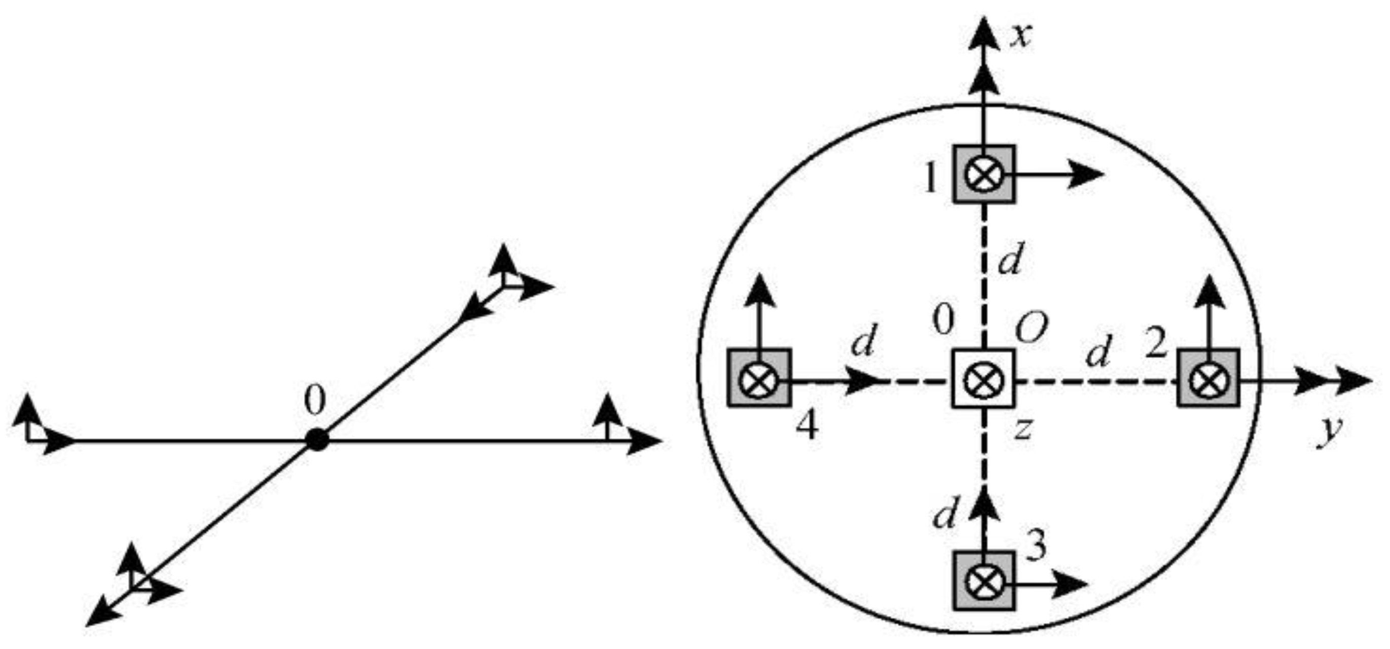
Here we briefly introduce the theory of magnetic anomaly especially the magnetic gradient tensor, and derive the analytical formula of the magnetic gradient tensor and other quantities based on the four-flux gate sensor cross array detector, shown in Figure 1.
Equation (1) represents the relationship between magnetic scalar potential , magnetic field vector, and magnetic gradient tensor. It is clear that the gradient tensor is symmetric and traceless, , so there are only five independent components in the gradient tensor matrix [3,4,5]. Equation (2) is used to derive total magnetic intensity (TMI) from the magnetic field vector [2,3,4,5]:
Figure 1 shows the four-flux gate sensor cross array detector we used, which is symmetrically placed. There is a fluxgate sensor in each of the four positions 1, 2, 3, and 4. We used the average value of four sensors (1, 2, 3, and 4) as the value of position O. From the three components () of the magnetic field vector measured by the flux gate directly, TMI can be solved according to Equation (2). TMI is calculated from the of position O. The magnetic gradient tensor algorithm is based on the flux gate position difference calculation. Taking the array of Figure 1 as an example, the formula of the magnetic gradient tensor matrix G is as follows [1,2,3,4,5]:
where represents the magnetic field vector of the flux gate sensor in direction and is the baseline distance.
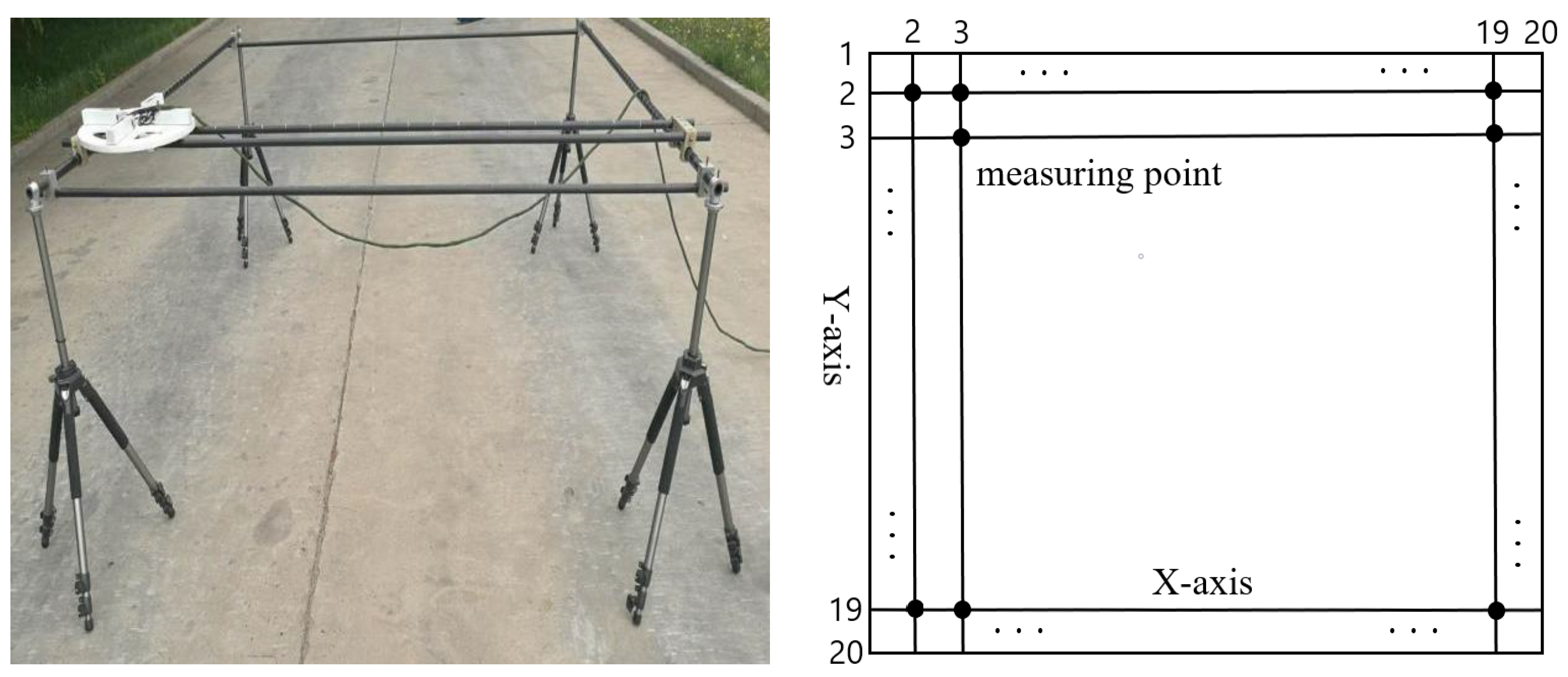
Figure 2 shows the design of the laboratory table, which is symmetric. It is a square plane with a length of 2 m and a measuring point set every 0.1 m. There are 20 scales on each side, with a total of 20 × 20 measuring points. The design of the laboratory table is like a 20 × 20 grid. The measured data are like a 20 × 20 square matrix. We can detect the data of each point by moving the flux gate sensors (the white device in Figure 2) on the bench. It will take half an hour to detect an original signal.
Because every point detected by the flux gate sensors contains the information of the three components ( ) of the magnetic field vector, which are detected by the flux gate sensors directly, the magnetic gradient tensor matrix for each point can be calculated by Equation (3). In addition, TMI for each can be calculated according to Equation (2). Eventually, nine 20 × 20 square matrices based on nine conponent signals including total magnetic intensity (TMI), the three components () of the magnetic field vector, and five tensor matrix independent elements () [1,2,3,4,5] can be separated from the original signals.
3. Discrete Wavelet Transform
We briefly introduce the theoretical basis of DWT. Some information is from Wikipedia.
Discrete wavelet transform (DWT) is a new analysis method that can localize the analysis of time (space) frequency. It can automatically adapt to the needs of time-frequency analysis, so it can focus on any detail of the signal and solve the difficult problem of Fourier transform, becoming a major breakthrough in scientific methods since the Fourier transform [25]. For magnetic anomaly signals detected by the flux gates, it must contain the noise of the magnetic background field and the mixture of other large ferromagnetic objects in the background. Therefore, before we extract the features of the two-dimensional signal, we must first reduce its noise, otherwise a large amount of information will be submerged in the noise. The frequency of the geomagnetic signal is low, while the frequency of the noise is high, and the two are closely mixed so it is not easy to separate them. The DWT method, which is more suitable for analyzing this variety of local frequency band, is used here. DWT noise reduction can support significant signal spikes as well as abrupt signals [26,27,28]. So wavelet transform is used to eliminate static in transient signals and suppress disturbance from high-frequency noise, and discrete wavelets are used to eliminate static in two-dimensional signals [25,26,27,28,29].
There are finest time frequency position characteristics in discrete wavelet transform, and their linear representation is: , which retains the wavelet coefficients mainly controlled by the signal, and finds and removes the wavelet coefficients controlled by noise (as in threshold processing). The remaining wavelet coefficients are inversely transformed to obtain the denoised signal.
The dispersed wavelet transform [30] from signal is calculated by passing it through a series of filters. Primarily these specimens pass through one low-pass filter within pulse response , leading to the curl of both:
The high-pass filter is used to disintegrate concurrent signals. The production provides particular quantities (high-pass) and similar quantities (low-pass). It is worth noting that the high-pass and low-pass filters are interrelated in what is called a quadrature mirror filter. Duplicating this decomposable process can add immense frequency resolution and the similar quantities disintegrate into two kinds of filters, which are then downsampled. It can be referred to as a binary tree or a filter bank, that has panel joints showing subspace with diverse time frequency localization.
The signal disintegrates into two kinds of frequencies in every process. As a result of decomposable procedures, this input signal should be and times to express the quantity of levels. At the same time, these procedures are at half time resolution because every filter output has 50% of the signal character, but every output has 50% of input frequency band, therefore we can use the subsampling operator to duplicate the frequency resolution [31].
Thus the implementation of the filter bank’s wavelets can be expressed as calculating the wavelet modulus of discrete units of subclass wavelets for the known superclass wavelet . In terms of the discrete wavelet transform, the superclass wavelet is transformed as well as proportioned through the energy of both:
where refers to the proportion parameter and refers to the shift parameter, and they are integers [25,26,27,28,29].
Evoking the wavelet modulus of signal refers to the prediction of to a wavelet, making a signal of distance . In terms of a subclass wavelet in the upper discrete group:
Arrange at a certain proportion; refers to a sigma function of alone [32]. According to the upper equality, can be seen as the convolution of including the superclass wavelet’s addition with spreading, reflection, and standardization, and catches samples at panel joints . However, it is apparent that this detail of coefficients supports level of the discrete wavelet transform. Thus for a suitable selection of and , this particular modulus of this filter group is in accordance with the wavelet modulus of a discrete group of subclass wavelets for the existing superclass wavelet [25,26,27,28,29].
There are mature DWT noise reduction algorithms in Matlab. We have carried out experiments in Matlab to prove the DWT noise reduction of geomagnetic signals.
4. Local Binary Pattern Feature
For symmetric signals, the local binary pattern feature can better represent the signal information. LBP refers to a kind of optical descriptor applied for categorizing in computer vision, i.e., an operator applied to express the partial structure characters of an image that has the characteristics of multiresolution, constant grayscale, and constant rotation. It is mainly used for texture extraction in feature extraction [33,34,35,36,37].
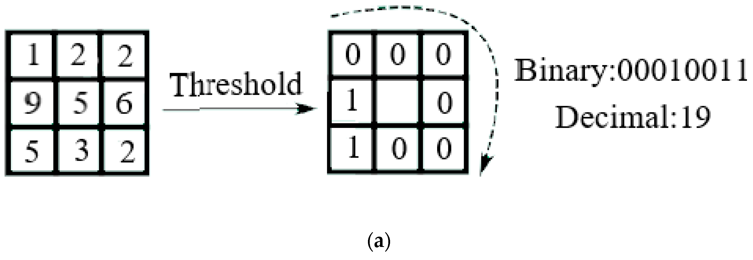
The initial LBP operator is interpreted within the vicinity of the 3 × 3 picture element, with the neighborhood key picture element as doorway, and the gray values of the close eight-picture elements are contrasted with the picture element values of the neighborhood center, and when the circumjacent pixels are bigger than that central picture element volume, the location of the picture element is designated as 1, otherwise 0.
Thus, eight points in the 3 × 3 vicinity are contrasted to generate eight-bit binary encodings, and the eight-bit binary encodings are sequentially arranged to form one binary number [37,38,39], as shown in Figure 3. This binary number is the LBP volume of the key picture element, and the LBP volume has possibilities. Therefore, there are 256 LBP values. The LBP volume of the key picture element reflects the texture information of the area around the pixel. The above process can be represented by an image, as in Figure 3 [33,34,35,36,37,38,39,40,41].
The LBP character vector is made as follows:
Start
Step 1: The examined window will be separated into cells, for example, 16 × 16 picture elements in every cell.
Step 2: Regarding every picture element in one cell, contrast the picture element with each of its eight neighbors (such as positions on upper left, middle left, left lower, upper right, and so on). Align the picture elements along a circle, for example, clockwise or anticlockwise. See Figure 3 for details.
Step 3: If the neighbor’s volume is smaller than the key picture element’s volume, it is designated as 0; otherwise 1. This provides an eight-digit binary encoding (always conveniently transform to decimal system).
where is the key picture element within strength and is the strength of the interpreted picture element. refers to the blip facility, explained as follows:
Step 4: Count the column diagram, through the cel, of the vibrational frequency of every “figure” coming out, for example, every mixture of picture elements that are smaller or bigger than the key. The column diagram can be 256-dimension character vectors.
Step 5: Alternatively regularize the column diagram.
Step 6: Conjoin the (regularized) column diagrams of all cells. This provides a character vector for the complete window.
End
Next we will perform feature analysis to verify the classification effect of LBP features.
5. Simulation and Analysis
To prove the feasibility of the LBP feature in the classification, we simulated the process of feature extraction. We establish six magnetic anomaly models of one magnetic source with six different orientations in MATLAB. The format of the simulation data is the same as that measured by the device shown in Figure 1 and Figure 2, which are 20 × 20 matrices, as in Figure 4. The six orientations are our target to classify using SVM.
The magnetic source of six models is the same cylinder with a length of 1 m and a diameter of 0.2 m, with relative magnetic permeability setting to 4000 in MATLAB, and the theory and equations come from reference [42]. It is in a depth of 2 m. We set all the six to vertical magnetization, and only the orientations are different and the rest of the conditions are the same, and the orientation conditions are shown in Table 1. Since we have analyzed the noise in Figure 5, we are not adding noise again in the simulation.
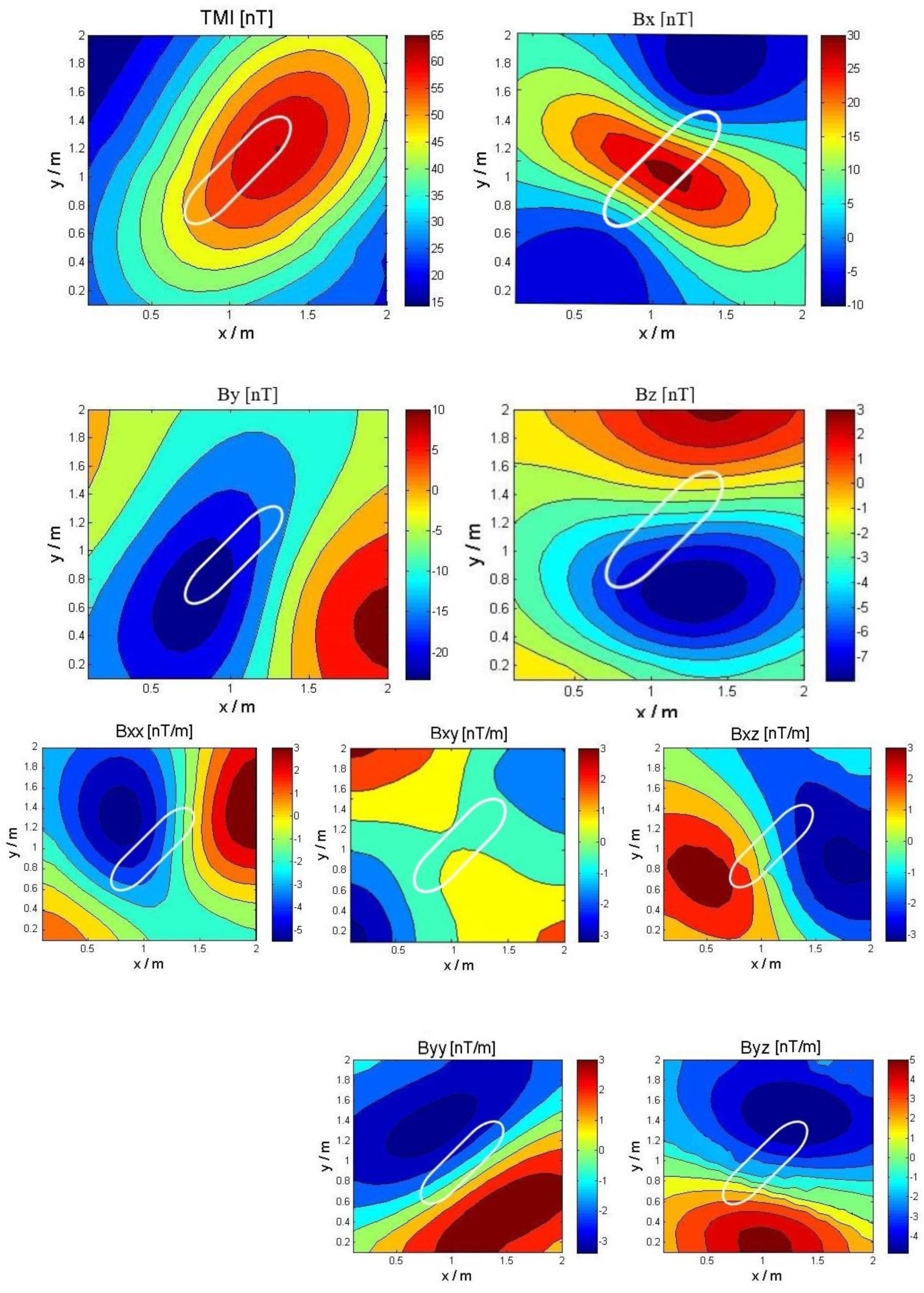
Taking type 1 as an example, Figure 4 shows the nine component signals. We can see from the figure that the magnetic anomaly signal of the symmetrical ferromagnetic object has good symmetry, which has great advantages for the signal processed later. Typical and obvious image features like those symmetrical textures in the image also facilitate pattern recognition. We can use this diagram to have an intuitive understanding of the signals to be processed.
The angle of inclination is the angle between the central axis of the cylinder and the x-y plane, and the downward direction is positive. The declination is the angle between the central axis of the cylinder and the x-axis, and the counterclockwise direction is positive.
The purpose of our simulation is to analyze the classification ability and effect of the LBP feature of the orientations and verify the feasibility of the above method. Feature selection is one of the key steps in SVM. The pros and cons of selected features directly affect the classification results. We define two kinds of feature classification ability: interclass discrimination, which is the degree of feature dispersion between classes, the larger the better; and intraclass aggregation, which is the degree of feature aggregation within classes, the greater the better [43,44].
Then, we extracted the LBP features of the nine component signals of the six orientations and analyzed their classification effects.
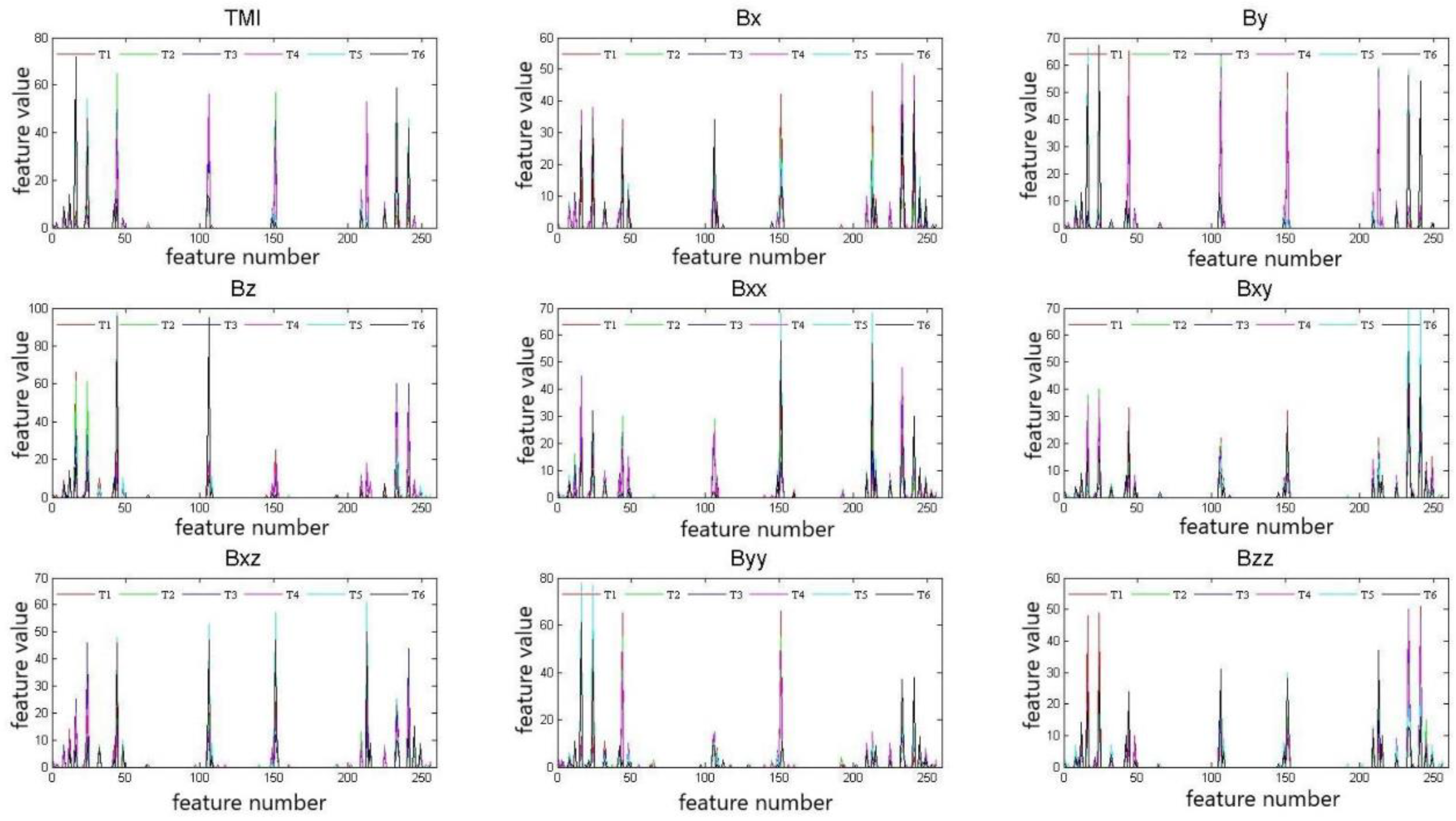
Each component signal’s LBP is a one-dimensional vector, and the length depends on the number of LBP features, and we can extract 256 values from each component as features. Here, we have a 9 × 256 matrix of features relative to each orientation. It can be seen in Figure 5 and Figure 6 that the LBP features of the nine component signals have good interclass discrimination and intraclass aggregation [43,44,45].
We can judge whether a feature has the ability to classify different orientations by observing the aggregation and dispersion of the data. In Figure 5, each line in a different color is a type of orientation. This image is an analysis of the LBP from the perspective of each component signal, which illustrates the distinguishing of the six orientations’ LBP feature of the different components. T1 is Type 1, T2 is Type 2, and so on. The numerical value of the vertical axis in the figure represents the LBP features, and the horizontal axis represents the number of 256 features. The more different the feature values, the better the classification performance. It can be seen that although there is some confusion, six types can be distinguished. The combination of the nine components aims to eliminate confusion as much as possible and improve the accuracy of classification.
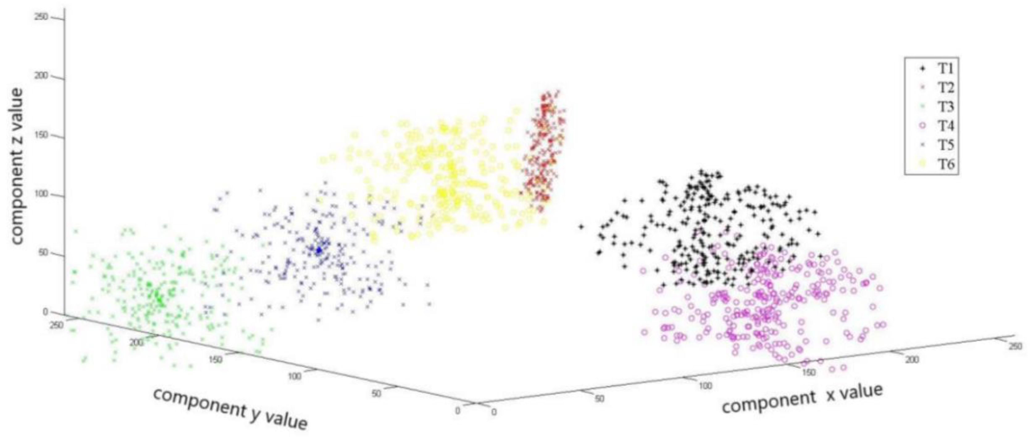
In Figure 6, points of each color represent a type of LBP feature data that is made up of three components signals (the axes each represent a component signal) of each orientation. The three kinds of components are randomly selected, and a three-dimensional scattergram is established. The purpose is to visually observe the classification effect of these nine attributes to distinguish the six orientations. It can be seen that the LBP feature data of the six orientations are obviously different, although there is still a small intersection, but it does not greatly affect the classification. In sum, the LBP data show an ability to identify different orientations. We can obviously see the dispersion and aggregation between classes, which means the LBP data of the same orientation get together. In contrast, the LBP data of different orientations are separated into parts. So we can conclude that the LBP features of the different orientations can be used to identify the symmetrical magnetic objects.
Where, for example, the LBP values of are 2, 3, and 4, respectively, so the corresponding point coordinates are (2, 3, 4). We can get all points like this. Similarly, the three component signals’ LBP features, which have the sum 3 (components) × 6 (orientations) × 256 (features), are in the three-dimensional system of coordinates in Figure 7.
6. Experimental Verification
In order to prove the feasibility of the method, an experiment was conducted using the experimental table and four-flux gate sensor cross array detector shown in Figure 1 and Figure 2. The target is a solid steel cylinder 1 m long and 20 cm in diameter at a horizontal depth of 1 m.
First, the same six orientations as the simulation were set (see Table 1 for details). At our experimental location, the magnetic inclination angle was 55°, the magnetic declination was −9°, and the classification labels were set to 1, 2, 3, 4, 5, and 6. In this paper, in order to not be redundant, only six orientations were designed for experiment. We only prove the feasibility of this method in theory. In practical engineering applications, the more the training samples of orientations constructed, the more the orientations which can be recognized. It can theoretically recognize any unknown object as long as the training sample is sufficient. Until any unknown orientation or size is detected. This is the basic theory of pattern recognition. In the support vector machine, the classification result is represented by an integer, with the number 1 representing type 1 orientation, and so on. After the nine component signals were separated according to the method mentioned above, they were subjected to wavelet denoise processing.
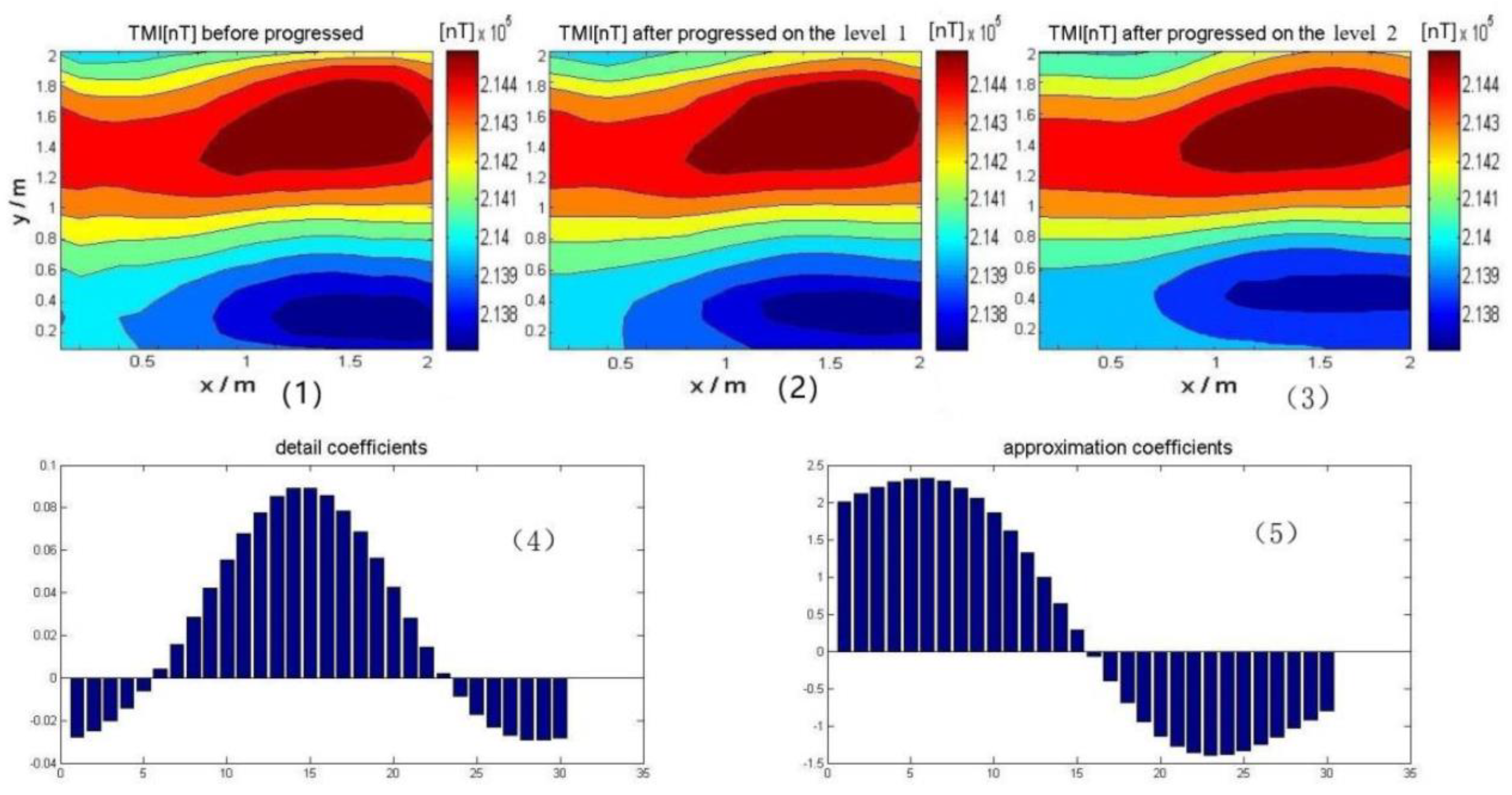
To prove the effect of this DWT noise reduction, Figure 7 shows the TMI image, which is calculated from the original signal detected by our detector at the orientation of Type1 in experiment, before and after noise reduction. Just only use TMI data as an example for analysis. Figure 7 shows TMI from our target placed parallel to the x-axis of the experiment table. We detected the three components () of the magnetic field vector through flux gate sensors, and calculated TMI by Equation (2). According to the figure, we know that this initial magnetic anomaly signal contains a lot of noise and interference. Discrete wavelet transform can effectively reduce the noise and make the signal clearer and more obvious. Of course, the different decomposition levels have different effects. We compared the signal-to-noise ratio (SNR) under two conditions, which is shown in Equation (10). We can conclude that when the level is 1, the SNR is equal to 44.3 (dB) and when the level is 2, the SNR is equal to 57.2 (dB). We can get the same opinion on the image. When the level is 2, the denoising effect is smoother and better, so we chose level 2.
where the is the signal before DWT, and is the signal after DWT. The bigger the SNR, the better the noise reduction effect.
As an example, Figure 8 shows images of the nine components of magnetic anomaly after wavelet processing of just one type of orientation. The other five orientations are similar to those in Figure 8.
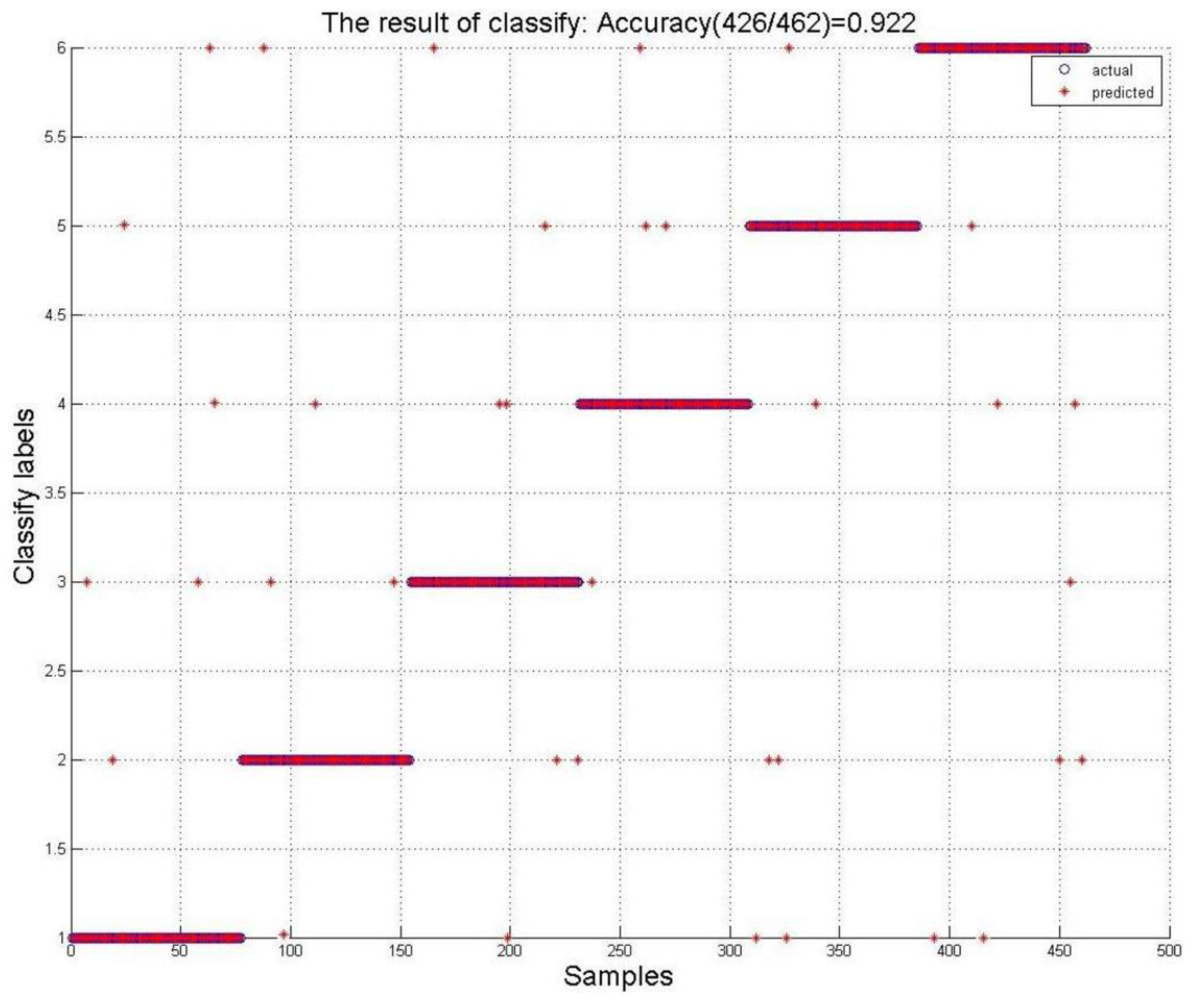
Then, the experimental signal’s LBP features were then extracted and constructed as a feature vectors. We use experimental data to train the support vector machine and use other experimental data to test the classifier. We have a 9 × 256 matrix of features relative to each orientation. Because we set 6 orientations, we have a 9 × 1536 features vector. Every column (9 × 1) is a sample which corresponding to a label. We have 1536 samples. The construction of the support vector machine requires a training sample to train the classification network, and verification of the classification requires a test sample. So we divided feature vectors into training samples and test samples according to a classic ratio of 7:3. We have 1074 training samples to train the SVM and use 462 test samples to predict the six orientations. Each sample (including training samples and test samples) corresponds to a label (1, 2, 3, 4, 5, 6). The training sample is to enable the SVM to establish a network of relationships between samples and labels, for example, if input the samples of type 1, the SVM will only output the label 1; while input the samples of type 2, the SVM will output the label 2. After that, we input the test sample into the SVM and we get a set of labels from trained SVM. The test samples itself also have a set of labels. The comparison of the two sets of labels from the test samples is shown in Figure 9. It shows the classification effect of the SVM. In practical applications, the data of the unknown object we detect are equivalent to the test samples. In Figure 9, the result of classify based on the test samples is displayed. The actual labels are their own labels, and the predicted labels are the output of the SVM trained by the training samples. The comparison of actual labels and predicted labels can prove the accuracy.
The SVM was constructed using the training samples described above, and the test samples were classified using the SVM. The SVM predicts the test sample and compares the predicted result with the actual result to obtain the correct rate of classification, as shown in Figure 9.
According to the classification results, the experiment proves that this method has a high accuracy rate in the object orientation recognition of underground magnetic anomalies.
7. Conclusions
(1) We introduce machine learning into the field of symmetric magnetic object recognition. Using the support vector machine to identify the underground objects’ orientation, a good recognition effect is achieved, and the formula derivation and analytical calculation of a large amount of magnetic measurement data are avoided.
(2) The nine component signals of the magnetic anomaly are extracted to identify symmetric magnetic objects, and the magnetic anomaly data are further processed by discrete wavelet transform, which compensates for the lack of accuracy of certain magnetic data, improving data quality. Also, we extract LBP features and prove that it can be used in 2D magnetic anomaly signals.
(3) This paper only introduces a way of thinking to identify the orientation of symmetric magnetic objects. This paper only establishes a classification identification of an object and six orientations to prove the feasibility of this method in theory. For engineering applications it is not enough. This paper only provides an idea. In engineering applications, we can collect more training samples to identify more targets. We can detect small shallow targets by building a database (including hundreds of kinds and thousands of orientations) or enough training samples rather than magnetic model and magnetic field inversion or calculation. This is also the idea of pattern recognition.
Author Contributions
Conceptualization, J.Z.; methodology, H.F.; software, J.Z.; formal analysis, Q.Z.; investigation, J.Z.; resources, Z.L.; writing—original draft preparation, J.Z.; writing—review and editing, J.Z.; visualization, Z.L.; supervision, H.F.; project administration, H.F.
Funding
This research received no external funding.
Acknowledgments
Thanks to Gang Yin for some ideas.
Conflicts of Interest
The authors declare no conflict of interest.
References
- Reid, A.B.; Allsop, J.M.; Granser, H.; Millett, A.J.; Somerton, I.W. Magnetic interpretation in three dimensions using Euler deconvolution. Geophysics 1990, 55, 80–91. [Google Scholar] [CrossRef]
- Nara, T.; Suzuki, S.; Ando, S. A Closed-Form Formula for Magnetic Dipole Localization by Measurement of Its Magnetic Field and Spatial Gradients. IEEE Trans. Magn. 2006, 42, 3291–3293. [Google Scholar] [CrossRef]
- Yin, G.; Zhang, Y.; Li, Z. Geometric invariants of magnetic dipole gradient tensor and its application. J. Geophys. 2016, 59, 749–756. (In Chinese) [Google Scholar]
- Beiki, M.; Clark, D.A.; Austin, J.R.; Foss, C.A. Estimating source location using normalized magnetic source strength calculated from magnetic gradient tensor data. Geophysics 2012, 77, J23–J37. [Google Scholar] [CrossRef]
- Schmidt, P.W.; Clark, D.A. The magnetic gradient tensor. Geophysics 2006, 25. [Google Scholar] [CrossRef]
- Luo, Y.; Wu, M.P.; Wang, P. Full magnetic gradient tensor from triaxial aeromagnetic gradient measurements: Calculation and application. Appl. Geol. 2015, 12, 283–291. [Google Scholar] [CrossRef]
- Vuuren, L.J.J.V.; Kilian, A.; Phiri, T.J. Implementation of an unshielded SQUID as a geomagnetic sensor. In Proceedings of the 2013 Africon, Pointe-Aux-Piments, Mauritius, 9–12 September 2013. [Google Scholar]
- Rim, H.; Park, Y.S.; Jung, H.K. Interpretation of magnetic gradient tensor for automatic locating adipole source. ASEG Ext. Abstr. 2012, 2012, 1. [Google Scholar]
- Florio, G.; Fedi, M.; Pasteka, R. On the application of Euler deconvolution to the analytic signal. Geophysics 2006, 71, L87–L93. [Google Scholar] [CrossRef]
- Benhur, A.; Siegelmann, H.T.; Horn, D. A Support Vector Clustering Method. In Proceedings of the International Conference on Pattern Recognition, DBLP, Barcelona, Spain, 3–8 September 2000. [Google Scholar]
- Cristianini, N.; Shawetaylor, J. An Introduction to Support Vector Machines and Other Kernel-based Learning Methods; Cambridge University Press: Cambridge, UK, 2000. [Google Scholar]
- Decoste, D.; SchLkopf, B. Training Invariant Support Vector Machines. Mach. Learn. 2002, 46, 161–190. [Google Scholar] [CrossRef] [Green Version]
- Ehret, B. Pattern recognition of geophysical data. Geoderma 2010, 160, 111–125. [Google Scholar] [CrossRef]
- Christopher, J.C.B. A Tutorial on Support Vector Machines for Pattern Recognition. Data Min. Knowl. Discov. 1998, 2, 121–167. [Google Scholar]
- Rosati, I.; Cardarelli, E. Statistical pattern recognition technique to enhance anomalies in magnetic surveys. J. Appl. Geophys. 1997, 37, 55–66. [Google Scholar] [CrossRef]
- Keskes, N. Image analysis techniques for seismic data. SEG Tech. Program Expand. Abstr. 1949, 48, 443. [Google Scholar]
- Scollar, I.; Weidner, B.; Segeth, K. Display of archaeological magnetic data. Geophysics 1986, 51, 623–633. [Google Scholar] [CrossRef]
- Kowalik W, S. Image processing of aeromagnetic data and integration with Landsat images for improved structural interpretation. Geophysics 2012, 52, 875–884. [Google Scholar] [CrossRef]
- Maklad, M.S.; O’Regan, R.; Dilay, A. Pattern Recognition: Theory and Application to Reservoir Identification. SEG Tech. Program Expand. Abstr. 1993, 12, 75. [Google Scholar]
- Huang, D.; Clark, R.A.; Whaler, K.A. Advantages of Using Pattern Recognition Technique for Automatic Division and Classification of Regional Potential Field. EAEG Meeting. 1994. Available online: http://www.earthdoc.org/publication/publicationdetails/?publication=12636 (accessed on 7 December 2018).
- Kerr, J.D.; Abatzis, I.; Reeve, J. An investigation into the Practical Use of Image Processing Software for the Interpretation Geophysicist. EAEG Meeting. 1994. Available online: www.earthdoc.org/publication/publicationdetails/?publication=12574 (accessed on 7 December 2018).
- Haralick, R.M.; Shanmugam, K.; Dinstein, I. Textural Features for Image Classification. Cybern. IEEE Trans. Syst. Man 1973, 3, 610–621. [Google Scholar] [CrossRef] [Green Version]
- Ojala, T.; Harwood, I. A Comparative Study of Texture Measures with Classification Based on Feature Distributions. Pattern Recognit. 1996, 29, 51–59. [Google Scholar] [CrossRef]
- Ojala, T.; Pietikainen, M.; Harwood, D. Performance evaluation of texture measures with classification based on Kullback discrimination of distributions. In Proceedings of the 12th International Conference on Pattern Recognition, Jerusalem, Israel, 9–13 October 1994. [Google Scholar]
- Akansu, A.N.; Serdijn, W.A.; Selesnick, I.W. Emerging applications of wavelets: A review. Phys. Commun. 2010, 3, 1–18. [Google Scholar] [CrossRef]
- Liu, J. Shannon wavelet spectrum analysis on truncated vibration signals for machine incipient fault detection. Meas. Sci. Technol. 2012, 23, 279–282. [Google Scholar] [CrossRef]
- Bruns, A. Fourier-, Hilbert- and wavelet-based signal analysis: Are they really different approaches? J. Neurosci. Methods 2004, 137, 321–332. [Google Scholar] [CrossRef] [PubMed]
- Malmurugan, N.; Shanmugam, A.; Jayaraman, S.; Chander, V.D. A New and Novel Image Compression Algorithm Using Wavelet Footprints. Acad. Open Int. J. 2005, 14, 1–5. [Google Scholar]
- Broughton, S.A.; Bryan, K. Discrete Fourier Analysis and Wavelets: Applications to Signal and Image Processing, 2nd ed.; Wiley: Hoboken, NJ, USA, 2008. [Google Scholar]
- Kumar, B.; Yadav, A. Wavelet singular entropy approach for fault detection and classification of transmission line compensated with UPFC. In Proceedings of the IEEE 2016 International Conference on Information Communication and Embedded Systems (ICICES)–Chenai, Tamilnadu, India, 25–26 February 2016; pp. 1–6. [Google Scholar]
- Gao, C.; Huang, S.; Wang, H. Short-term Load Forecasting for Microgrids Based on Discrete Wavelet Transform and BP Neural Network. Open Electr. Electron. Eng. J. 2014, 8, 738–742. [Google Scholar] [CrossRef]
- Poularikas, A.D. Handbook of Formulas and Tables for Signal Processing. Math. Proc. Camb. Philos. Soc. 1998, 74, 55–81. [Google Scholar]
- He, D.C.; Wang, L. Texture Unit, Texture Spectrum and Texture Analysis. In Proceedings of the Geoscience and Remote Sensing Symposium, Igarss’89, Canadian Symposium on Remote Sensing, 1989 International; IEEE: Piscataway, NJ, USA, 1990; pp. 2769–2772. [Google Scholar]
- Silva, C.; Bouwmans, T.; Frelicot, C. An eXtended Center-Symmetric Local Binary Pattern for Background Modeling and Subtraction in Videos Visapp. In Proceedings of the International Joint Conference on Computer Vision, Imaging and Computer Graphics Theory and Applications, Berlin, Germany, 11–14 March 2015. [Google Scholar]
- Bouwmans, T.; Silva, C.; Marghes, C. On the role and the importance of features for background modeling and foreground detection. Comput. Sci. Rev. 2016, 28, 26–91. [Google Scholar] [CrossRef]
- Barkan, O.; Weill, J.; Wolf, L.; Aronowitz, H. Fast High Dimensional Vector Multiplication Face Recognition. In Proceedings of the IEEE International Conference on Computer Vision, Sydney, Australia, 1–8 December 2013. [Google Scholar]
- Liao, S.; Zhu, X.; Lei, Z. Learning Multi-scale Block Local Binary Patterns for Face Recognition. In Advances in Biometrics; DBLP; Springer: Berlin, Germany, 2007; pp. 828–837. [Google Scholar]
- Ahonen, T.; Hadid, A.; Pietikainen, M. Face Description with Local Binary Patterns: Application to Face Recognition. IEEE Trans. Pattern Anal. Mach. Intell. 2006, 28, 2037–2041. [Google Scholar] [CrossRef] [PubMed]
- Trefný, J.; Matas, J. Extended Set of Local Binary Patterns for Rapid Object Detection. In Proceedings of the Computer Vision Winter Workshop, Nove Hrady, Czech Republic, 3–5 February 2010. [Google Scholar]
- Zhao, G.; Pietikãinen, M. Dynamic texture recognition using local binary patterns with an application to facial expressions. IEEE Trans. Pattern Anal. Mach. Intell. 2007, 29, 915–928. [Google Scholar] [CrossRef] [PubMed]
- Heikklä, M.; Pietikäinen, M. A texture-based method for modeling the background and detecting moving objects. IEEE Trans. Pattern Anal. Mach. Intell. 2006, 28, 657–662. [Google Scholar] [CrossRef] [Green Version]
- Zhi-Kui, G.; Chao, C.; Chun-Hui, T. Forward modeling of magnetic anomalies of finite-length cylinder in 3D space. Chin. J. Geophys. 2017, 60, 1557–1570. [Google Scholar]
- Nguyen, M.H.; Torre, F.D.L. Optimal Feature Selection for Support Vector Machines. Pattern Recognit. 2010, 43, 584–591. [Google Scholar] [CrossRef]
- Chen, J.; Huang, H.; Tian, S. Feature selection for text classification with Naïve Bayes. Expert Syst. Appl. 2009, 36, 5432–5435. [Google Scholar] [CrossRef]
- Gheyas, I.A.; Smith, L.S. Feature subset selection in large dimensionality domains. Pattern Recognit. 2010, 43, 5–13. [Google Scholar] [CrossRef] [Green Version]
Figure 1.
Four-flux gate sensor cross array detector we used.

Figure 2.
Design of the experiment table which is like a 20 × 20 grid. The picture on the left is the real thing, the picture on the right is the schematic.
Figure 2.
Design of the experiment table which is like a 20 × 20 grid. The picture on the left is the real thing, the picture on the right is the schematic.

Figure 3.
(a) Basic principle of local binary patern (LBP); (b) three interpreted instances explain texture and count one LBP.
Figure 3.
(a) Basic principle of local binary patern (LBP); (b) three interpreted instances explain texture and count one LBP.


Figure 4.
Type 1 model’s nine component signals including total magnetic intensity (TMI), Bx, By, Bz, Bxx, Bxy, Bxz, Byy, Byz in MATLAB.
Figure 4.
Type 1 model’s nine component signals including total magnetic intensity (TMI), Bx, By, Bz, Bxx, Bxy, Bxz, Byy, Byz in MATLAB.

Figure 5.
This image is an analysis of the LBP from the perspective of each component signal, which illustrates the distinguishing of the six orientations’ LBP feature of the different components. T1 is the feature of Type 1, T2 is the feature of Type 2, and so on. We can compare the same and different characteristics of the six types in the figure. We aimed to analyze the classification ability of LBP features for 6 different orientations.

Figure 6.
The classification effect of three component signals to distinguish the six orientations in 3D.
Figure 6.
The classification effect of three component signals to distinguish the six orientations in 3D.

Figure 7.
Discrete wavelet noise reduction effects. (1) shows the TMI signal before discrete wavelet transform (DWT), (2) shows the TMI signal after DWT on the level 1, (3) shows the TMI signal after DWT on the level 2 and (4), (5) show the details of coefficients.
Figure 7.
Discrete wavelet noise reduction effects. (1) shows the TMI signal before discrete wavelet transform (DWT), (2) shows the TMI signal after DWT on the level 1, (3) shows the TMI signal after DWT on the level 2 and (4), (5) show the details of coefficients.

Figure 8.
Nine components signals after wavelet denoising in one orientation.

Figure 9.
Classification results.


Table 1.
Orientation conditions.
| Type | Inclination (°) | Declination (°) |
|---|---|---|
| 1 | 0 | 0 |
| 2 | 30 | 45 |
| 3 | 60 | 45 |
| 4 | 0 | 90 |
| 5 | 30 | −45 |
| 6 | 60 | −45 |
© 2019 by the authors. Licensee MDPI, Basel, Switzerland. This article is an open access article distributed under the terms and conditions of the Creative Commons Attribution (CC BY) license (http://creativecommons.org/licenses/by/4.0/).
Share and Cite
MDPI and ACS Style
Zheng, J.; Fan, H.; Li, Z.; Zhang, Q. Symmetric Magnetic Anomaly Objects’ Orientation Recognition Based on Local Binary Pattern and Support Vector Machine. Symmetry 2019, 11, 97. https://doi.org/10.3390/sym11010097
AMA Style
Zheng J, Fan H, Li Z, Zhang Q. Symmetric Magnetic Anomaly Objects’ Orientation Recognition Based on Local Binary Pattern and Support Vector Machine. Symmetry. 2019; 11(1):97. https://doi.org/10.3390/sym11010097
Chicago/Turabian StyleZheng, Jianyong, Hongbo Fan, Zhining Li, and Qi Zhang. 2019. "Symmetric Magnetic Anomaly Objects’ Orientation Recognition Based on Local Binary Pattern and Support Vector Machine" Symmetry 11, no. 1: 97. https://doi.org/10.3390/sym11010097
Note that from the first issue of 2016, this journal uses article numbers instead of page numbers. See further details here.