1. Introduction
Green Radio communication has received a lot of attention in the past few years with an aim to decrease the carbon foot print of wireless networks. It has been estimated that nearly 70% of the energy being used by cellular operators is on the radio part [
1] and around 9% of the global CO
emission is from the communication systems [
2]. In addition, one of the main concerns is the User Equipment (UE) battery, which has not shown progression at par with the Radio Access Technology (RAT). This phenomena is highly visible for the cell edge users that despite spending higher energy (due to high pathloss shadow fading and adjacent cell interference) are unable to achieve fair share of the radio resources. In this context, Green communications employing cooperative and fair resource allocation techniques can help in reducing the carbon footprint and increasing Energy Efficiency (EE).
Most of the existing wireless systems use Orthogonal Frequency Division Multiple Access (OFDMA) to distribute radio resources among UEs. One of the existing RAT to use OFDMA is Long Term Evolution-Advanced (LTE-A), which has a similar structure to its predecessor LTE. In LTE, each Resource Block (RB) is a time frequency grid element. The basic RB structure contains 15 subcarriers of 12 KHz each and a 10 ms frame. Each frame is subdivided into 10 subframes of 1 ms and each subframe is further divided into 2 slots of ms each. Each slot may contain 6 or 7 OFDM symbols depending on a normal or an extended cyclic prefix. The RB allocation can be changed after every Transmission Time Interval (TTI) based upon channel conditions or RB allocation algorithm. OFDMA offers flexibility of RBs Allocation to tailor user and network requirement, such as throughput, fairness, Energy EfficiencyEE, and Spectral Efficiency (SE). For example, in order to support higher peak data rates Carrier Aggregation (CA) is introduced to obtain wider bandwidth. Compared to LTE, CA in LTE-A can support maximum 5 adjacent/non-adjacent component carriers of maximum 20 MHz to achieve 100 MHz bandwidth.
In addition, LTE-A allows Layer 3 (L3) relays to be incorporated in the network that can decode and forward the data to a UE [
3]. This cooperative communication addresses EE and throughput of the cell edge users by providing channel diversity. As the network can only accommodate finite relays, their placement is, therefore, crucial to manage the overall throughput. The RB allocation between direct link that is Base Station (BS)–UE and two hop link that is (BS)–Relay Node (RN)–UE can be done independently or in a shared manner. In [
4], the authors have presented a thorough comparison of basic RB allocation schemes, which are Round Robin (RR), Proportional Fairness (PF), Maximum Throughput (MT), and Maximum Minimum (MM); they presented an alternating MT and PF based resource allocation scheme SAMM (abbreviated with Authors’ names) without considering any relay. The paper considered LTE system with a basic RB structure [
5], 5 MHz bandwidth with fixed 10 users that are uniformly placed from the BS. These schemes have been compared in terms of sum throughput, individual user throughput and fairness based on JFI (Jains fairness index). The SAMM scheme provides a better tradeoff between throughput and fairness. Cell edge users show some throughput gains due to proportional fairness, however, this scheme fails to address EE. Authors in [
6] considered EE for generic OFDMA based downlink system. They presented Bisection based Optimal Power Allocation (BOPA) algorithm for a given RB assignment. The BOPA works as an iterative approach based on water filling principle. This work uses equal power allocation among users for initial users’ rate calculation, whereas, a modified algorithm in [
7] uses equal power per resource block.
In [
8], the authors proposed a quality of service (QoS) aware optimization problem for relay-based multi-user cooperative OFDMA uplink system. The main goal is to find optimal solutions for relay selection, power allocation and subcarrier assignment that maximize the system throughput. Aiming to support and attain the green wireless LTE network, an energy-efficient resource allocation scheduler with QoS aware support for LTE network is proposed in [
9]. The authors of [
10] proposed a two-stage method to solve the inter-cell interference problem. In the first stage, the subcarrier allocation and time scheduling are jointly conducted with sequential users’ selection and without considering the interference. The power control optimization is left to the second stage, using a geometric programming method.
In [
11], energy efficient resource block and power allocation optimal and low complexity suboptimal schemes are presented for OFDMA relay-assisted downlink. Authors use fractional programming to make the non-linear mixed integer problem to convex subtractive problem. In order to reduce the computational complexity of the optimal solution, they present two-stage RB allocation and transmission power control algorithms. The system model of this paper is similar to our model but they use relays (small eNB in that paper) with frequency reuse factor of one, and the users employ maximal ratio combining to maximize the received signal-to-noise ratio (SNR). In our case, we use multiplexing gain instead of the diversity gain at users’ end by exploiting the knowledge of their location in relay selection and users association algorithm. We have compared our proposed schemes with the low complexity energy-efficient resource block and power allocation (LERPA) algorithm 3 and 4 of [
11].
Artificial intelligence techniques can be used in highly dynamic and stringent constraint Next-Generation networks. Since machine learning is a most promising technique of artificial intelligence, it can be directly/indirectly employed to achieve the goals of 5 G in cognitive radios, massive multiple-input multiple-output (MIMO), hybrid beamforming, femto/small cells, smart grid, wireless power transfer, device-to-device communications, non-orthogonal multiple access (NOMA) etc. [
12]. This paper [
12] gives an overview of the applications of machine learning in Next-Generation wireless networks. Specifically, supervised learning techniques are suitable for massive MIMO channel estimations and spectrum sensing, unsupervised learning could be helpful in users grouping and clustering; and reinforcement learning can be applied in resource allocation problems.
A detailed review on existing techniques and methods have been provided in [
13]. For example, in [
14], a cooperative Q-learning approach was applied as an efficient approach to solve the resource allocation problem in a multi-agent network. The quality of service QoS for each user and fairness in the network are taken into account and more than a four-fold increase in the number of supported small cells. The authors in [
15], proposed a machine learning framework for resource allocation to determine the optimal or near-optimal solutions based on the learning of the most similar historical scenario.
In paper [
16], the authors proposed an approximated solution to a wireless network capacity problem using flow allocation, link scheduling, and power control. The Support Vector Machine (SVM) was used to classify each link to be assigned maximal transmit power or be turned off, whereas, the deep belief networks (DBNs) computes an approximation of the optimal power allocation. Both learning approaches have been trained on offline computed optimal solutions. A novel resource allocation method using deep learning to squeeze the benefits of resource utilization was developed in [
17]. It was reported that when the channel environment is changing fast, the deep learning method outperforms traditional resource optimization methods. The resource allocation is to be optimized by a convolutional neural network using channel information. A similar problem has been explored in [
18] that use Upper Confidence Bound learning for Greedy Maximal Matching (GMM) when the channel statistics are unknown. Since the subchannel and power allocation problem is a non-convex combinatorial problem, the optimal solution of the subchannel and power allocation problem requires an exhaustive search over all possible combinations of subchannels and power levels. In order to train the deep neural network (DNN) for an optimal solution, Ref. [
19] utilizes the genetic algorithm to get the training data for DNN. It shows that the prediction accuracy increases with the size of dataset and the number of hidden layers. A four-step reinforcement learning based intercell interference coordination (ICIC) scheme is presented in [
20]. The users selection, resource allocation, power allocation, and retransmit packet identification are handled by reinforcement learning to reduce the intercell interference.
However, to the best of our knowledge no available literature discusses LTE-A with L3 relays for SE and EE consideration. In this work,
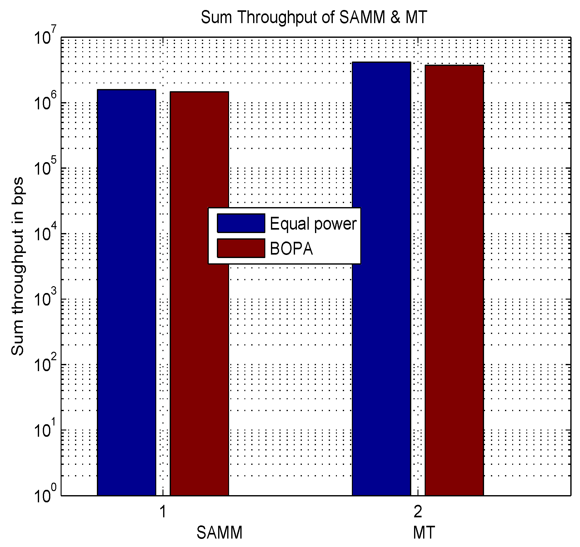
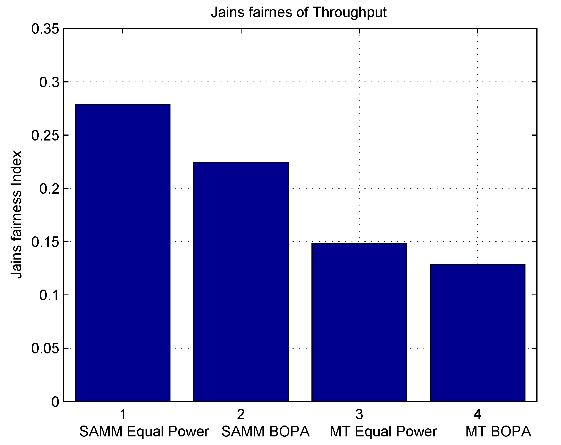
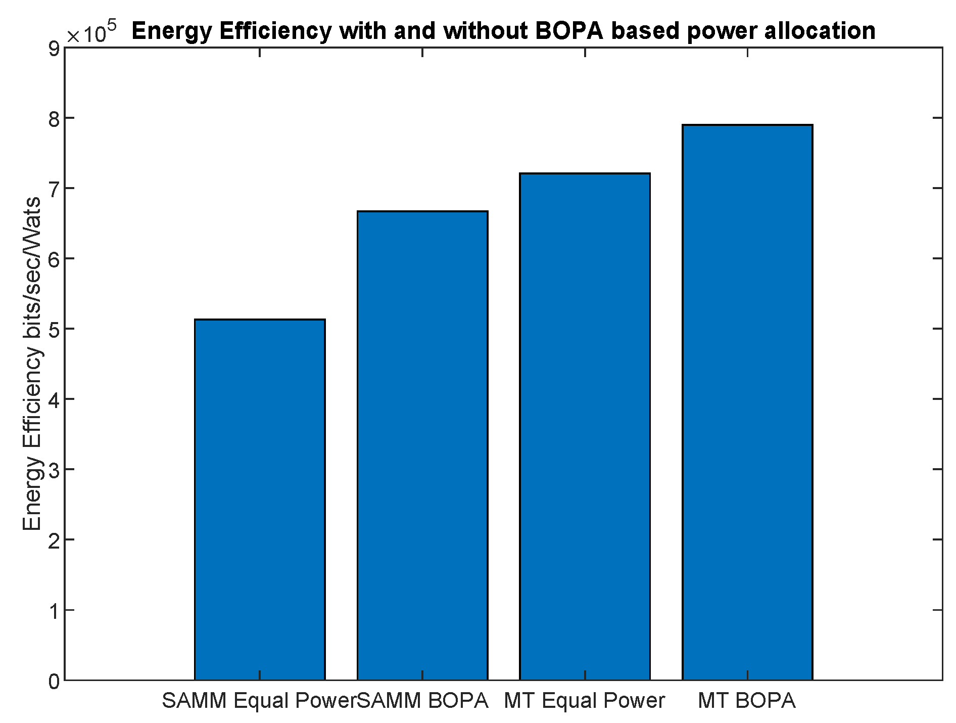
We present an energy efficient algorithm based on SAMM and BOPA for LTE-A system with a L3 relay. Performance evaluation in terms of throughput, fairness, power consumption, SE and EE is shown between two best performing schemes i.e., MT and SAMM considering equal power and BOPA.
Considering the practical deployment, where there may be more than one relay supporting the cell edge users, we devise a clustering strategy to obtain near optimal placement of L3 relays and users’ association.
In a multiple relay scenario, to optimize EE and reduce computational complexity of running algorithm every TTI, we present a two step machine learning process that uses both the SAMM and BOPA approach for resource and power allocation of the cell users. The proposed approach is compared to MT equal power, MT BOPA and SAMM equal power in terms of users’ throughput and EE.
A complete list of notations used in this paper is given in
Table 1.
Rest of the paper is organized as follows: system model is described in
Section 2, algorithms and performance for MT, SAMM and BOPA with single relay network are given in
Section 3. Multiple relay users’ association and deployment with machine learning based power and RB allocation for SAMM is presented in
Section 4. Complexity analysis is given in
Section 5, followed by the conclusions in
Section 6.
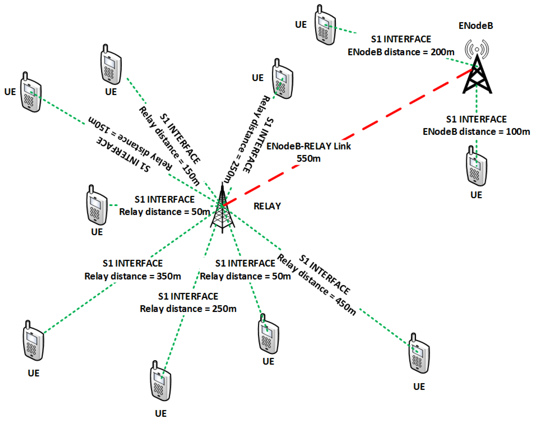
2. System Model
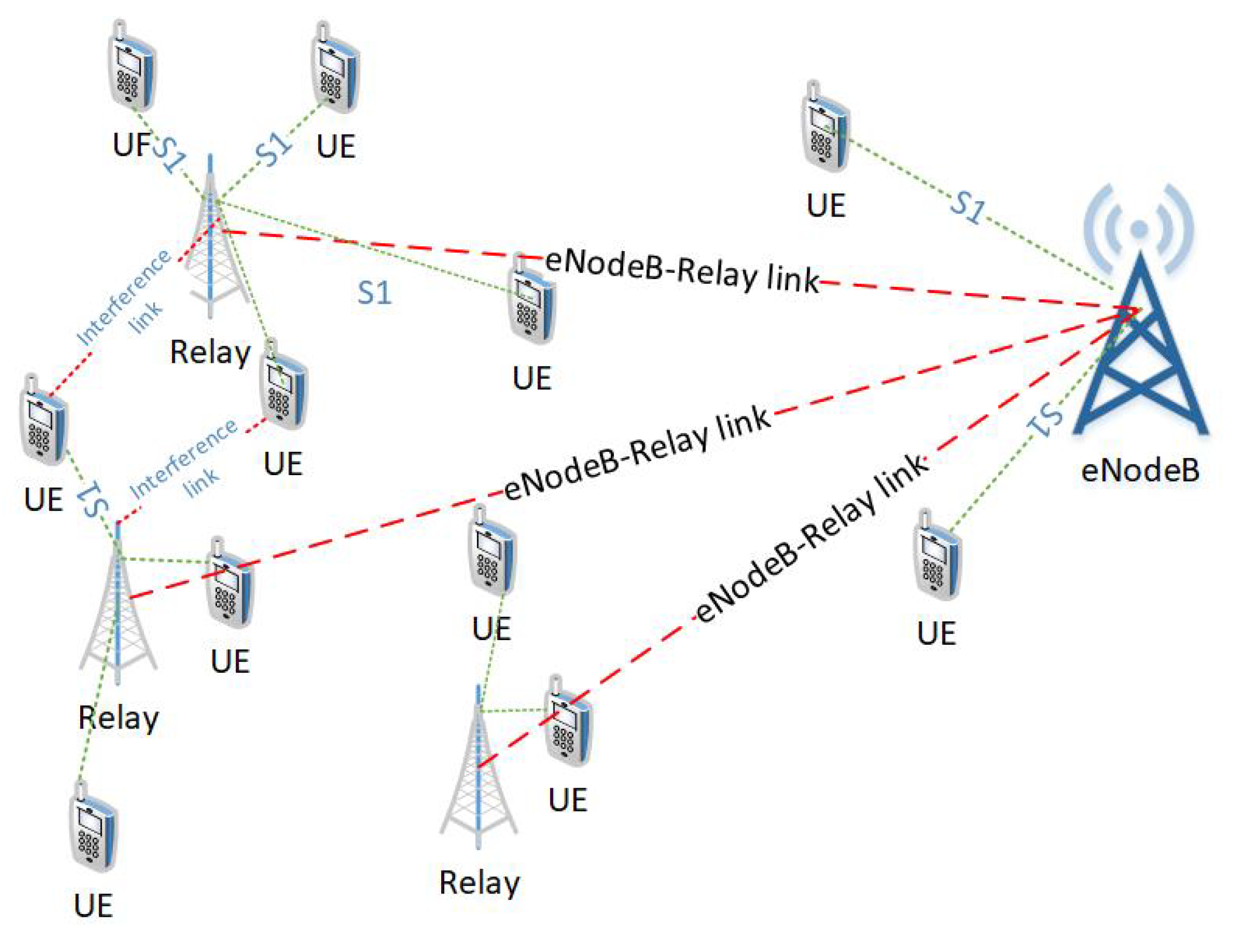
We consider a two-tier LTE-A system with a BS supported by L3 relays as shown in
Figure 1. The relays are assumed to be In-band type 1b [
3] and full duplex, placed in the center of BS to the most distant user. A total of
K users and
N RBs are considered with users placed at a uniform distance from BS. The total powers of BS and RN are denoted by
and
, respectively. The LTE-A system uses OFDMA transmission in the downlink. Let the system bandwidth is
B with
N number of RB, then,
is the bandwidth of one RB. We express the channel gains
and
for user
k where
on RB
n where
for BS and RN respectively. Practically, the channel gain depends upon various factors, including thermal noise at receiver, receiver noise figure, antenna gains, distance between transmitter and receiver, path loss exponent, log normal shadowing and fading. Therefore, for all the links, we can write
In the above equation,
(83.46 dB) is a constant depending upon thermal noise at receiver, receiver noise figure, and antenna gains,
is path loss exponent,
is the distance in Km from UE
k to the BS/relay,
(10.5 dB) is shadowing parameter modeled by a normally distributed random variable with standard deviation 8 dB, and
corresponds to the Rayleigh fading channel coefficient of user
k in subchannel
n [
21].
The throughput of user
k is given by,
where the factor
in access link shows the two time-slots transmission from BS-RN and RN-UE, and
is the binary variable such that
when RB
n is allocated to the user
k,
is the maximum average signal-to-noise ratio for user
k between direct and relay links. Let
be the signal-to-noise ratio for user
k via Direct Link, and
be the signal-to-noise ratio for user
k via Relay Link, then, the
is given as
where,
is
The Energy Efficiency EE in terms of
can be expressed as
The EE optimization problem for the above scenario can be written as
where
is the proportional rate constraint [
22]. We assume that channel state information (CSI) of all the users is known to the BS. Also, it is assumed that the RB allocation decision and assignment is done in less than channel coherence time so that CSI information can be used. This further puts constraints on the RB allocation algorithm complexity. The two-hop transmission to the RN users will be carried out in two TTI’s. In the first TTI, the BS will only send data to the RN users that are in close proximity of RN or have better RN-UE channel conditions than the direct link BS-UE. In the second TTI RN-UE data will be sent. BS will choose the path to the user (direct or via RN) with best channel coefficient in each TTI. The centralized scheduling minimizes the possibility of interference for In-band type of RNs. Frequency division duplexing ensures that the RN may handle backhaul data simultaneously with the access link data so that from the second TTI onwards backhaul BS-RN transmission is carried out simultaneously with the access link RN-UE transmission.
The LTE-A downlink is an OFDM based system which supports M-ary quadrature amplitude modulation (MQAM). We can use Equation (
2) to calculate the throughput of user
k on RB
n for both direct and relay-link paths. The two paths provide channel diversity to increase the users and system level throughput. We use MT and SAMM criteria for RB allocation with equal power allocation to all RBs or BOPA as explained below.
4. Fairness-Aware Machine Learning Based Power and RB Allocation with Multiple Relays
In practical scenarios, multiple relays are deployed to facilitate the cell-edge users as shown in the
Figure 7. The multiple relay deployment causes inter-relay interference. This interference can be minimized by the careful deployment of relays, transmit power control, and the scheduling of time/frequency resources. Though, L3 relays incur more processing delay as compared to the L1 and L2 relays but they provide robust transmission in the presence of interference [
26]. Assume there are
Q relays in a cell, such that relay
. The signal-to-interference-and-noise ratio (SINR) at UE
k in direct link is given as
where
is the transmit power of relay
q assigned to its associated user
and
is the channel gain between relay
q and the UE
k. Similarly, the SINR at UE
k in relay
q link is given as
As seen from the above equation, the interference and fairness causes a significant increase in the computational cost when deploying multiple relays. Therefore, we present a machine learning based approach that utilizes relay deployment and users’ association data to develop RB allocation and Power allocation strategy that maximizes the sum EE. Once trained, the proposed approach can save cost of scheduling in every TTI. This is shown in
Figure 8, the machine learning model takes the inputs: number of relays, relays’ coordinates, CSI, SNR, and total transmit power and produces the outputs: optimal relays’ coordinates with associated users, set of RBs assigned to each user
k, and the optimal power allocation (
) to each user
k in the RB
n. Based on single relay performance, the RB allocation block is trained using SAMM and power allocation block is trained using BOPA. Since the relay deployment can significantly alter the RB and power allocation, a clustering approach is presented that determines relay positioning and corresponding users’ association based on a pre-defined metric.
4.1. Relays Deployment and Users Association
In this section, we present an autonomous unsupervised machine learning scheme that provides users association with optimally deployed relay nodes in the cell-edge area. Machine learning algorithms can broadly be divided into two main categories, namely supervised learning and unsupervised learning algorithms. The former class of algorithms learn by training on the input labeled examples, called training dataset, , where the example consists of the instance of feature vector and the corresponding label . Given a labeled training dataset, these algorithms try to find the decision boundary that separates the positive and negative labeled examples by fitting a hypothesis to the input dataset. Unsupervised machine learning algorithms, on the other hand, are given an unlabeled input dataset. These algorithms are used for extracting information or features from the dataset. These features might be related, but not confined, to the underlying structures or patterns in the input data, relationships in data items, grouping/clustering of data items, etc. Discovered features are meant to provide a deeper insight into the input dataset that can subsequently be exploited for achieving specific goals. Clustering algorithms make an important part of unsupervised learning where the input examples are grouped into two or more separate clusters based on some features. The K-Means (KM) algorithm, is probably the most popular clustering algorithm. It is an iterative algorithm that starts with a set of initial centroids given to it as input. During each iteration, it performs the following two steps.
Assign Cluster: For every user, the algorithm computes the distance between the user and every centroid. The user is then associated to the cluster with the closest centroid. During this step, a user might change its association from one cluster to another one.
Recompute centroids: Once all users have been associated to their respective cluster, the new position of centroid for every cluster is then calculated.
Let us define the following notations to be used later in this section.
Now the cost function
J can be defined as
with the following optimization objective function.
It may be pointed out that Equation (
22) allows us to compare multiple clustering layouts based on their cost and select the one with the lowest cost.
In this section, we use the KM algorithm for optimal clustering of m users competing for resources in a particular cell. The clustering is performed based on their geographic location, thus our input dataset has m vectors , consisting of location coordinates, of ith user. For the sake of simplicity, we assume these users are deployed in a two dimensional area, i.e., a plane and so , i.e., an ordered pair of location coordinates. Our clustering algorithm is summarized in Algorithm 2.
The proposed algorithm takes the location coordinates of
m users as input. It also takes two numbers
and
as additional inputs. The algorithm outputs the best number of clusters,
k, such that
, and corresponding members of each cluster. It starts with
and randomly selects
k user locations as the initial centroids (line 6). It assigns the closest centroid to each user (line 8) and then computes new centroids by calculating the center/average location of all nodes in each cluster (line 11). So, in effect, the location of centroids keeps moving in successive iterations. It repeats the above two steps until the change in centroids’ positions is zero or negligible. We repeat the test
times with a new set of randomly chosen initial centroids every time. During every test, the discovered centroids, corresponding centroid assignment to users, and the cost are saved (lines 14–16) for later comparison. After running the loop for
times, we select and store the best
k centroids resulting from the test with the lowest cost while discarding the remaining (lines 19–21). The same is repeated for the next value of
k, i.e.,
, until
. At the end we have
vectors
, one for each value of
k, the corresponding assignment vector
and cost
. Finally, we choose the vector
having the lowest cost and corresponding assignment vector
among
stored cases. That is the best number of clusters and corresponding centroids that the algorithm found. A snapshot of the relay deployment and users’s association algorithm output is shown in
Figure 9.
| Algorithm 2 Users association clustering algorithm |
- 1:
- 2:
fordo - 3:
- 4:
for do - 5:
repeat - 6:
Randomly choose initial k centroids - 7:
for do - 8:
, such that is the centroid closest to - 9:
end for - 10:
for do - 11:
mean of all users/points assigned to centroid - 12:
end for - 13:
until converges - 14:
- 15:
- 16:
- 17:
end for - 18:
- 19:
- 20:
- 21:
- 22:
end for - 23:
- 24:
- 25:
- 26:
|
4.2. Resource Allocation by Multiclass Classification
The resource block allocation problem has multiple discrete outputs, i.e., the users, therefore, we use the multiclass classification to classify one out of
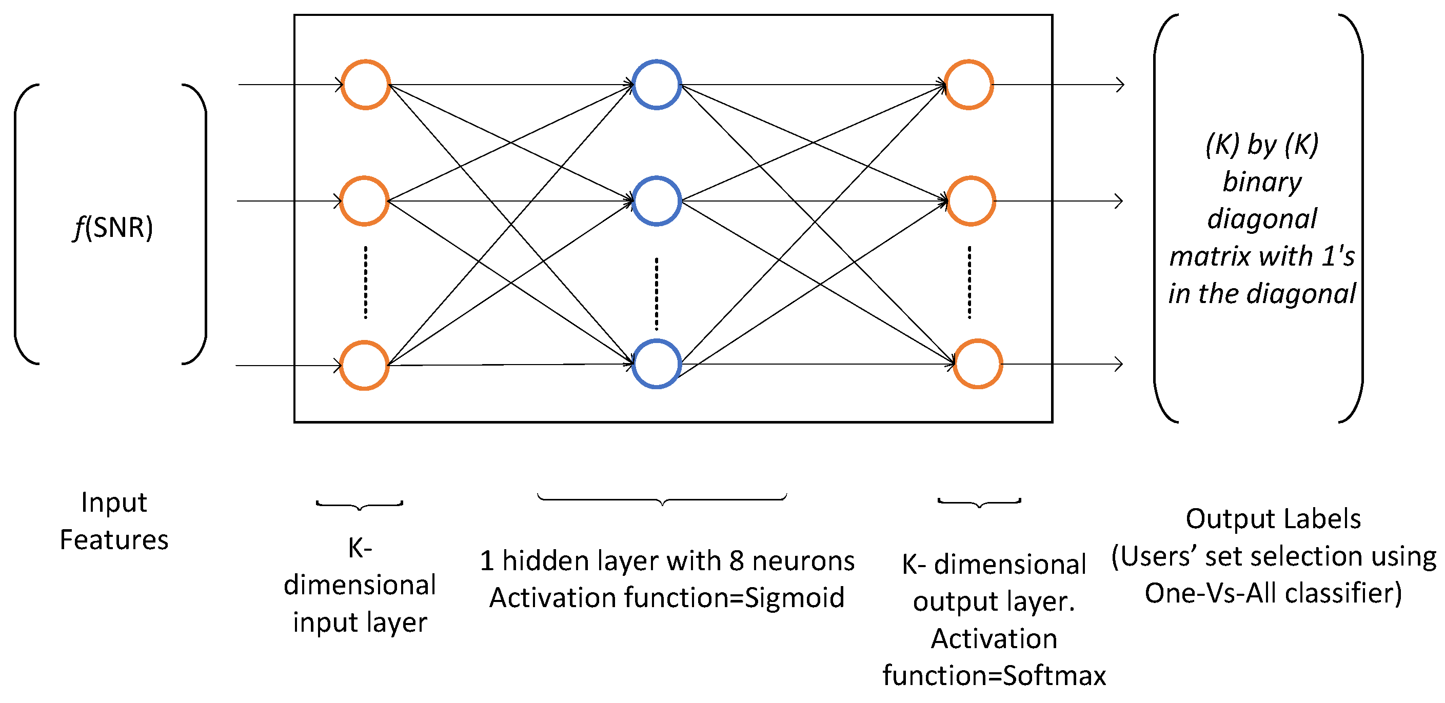
K users. The multiclass classification is an extension of One-Vs-All classification. The input of the training network comprises of channel state information in terms of the SNR and the output consists of a particular user that maximizes the utility function (throughput for MT and PF metric for the proportional fairness). The training data is obtained from the implementation of SAMM algorithm of [
4] as 25,000 K-dimensional samples of received SNR and the corresponding selected users. The dataset is partitioned into three parts, the training dataset, the validation dataset, and the test dataset. These are divided in 70%, 15%, and 15% ratio, respectively. The Matlab Neural Network Pattern Recognition Apps is used to train and deploy the neural network. It uses Scaled Conjugate Gradient algorithm [
27] for training. Our application requires
neurons in input layer and 10 neurons in output layer. A hit and trial choice of eight neurons in hidden layer gave the best result. The neural network architecture is shown in
Figure 10.
The neural network loss function is a generalization of the logistic regression’s loss function. In logistic regression classification problem, we try to find the weighted parameter
, such that the mean square error between the predicted output and the actual output is minimized. This is called loss function (LF) or the cost function and is given by
where the prediction or hypothesis function
is a sigmoid function, i.e.,
. In the above equation,
is a training dataset with
input-output pairs. However, loss function with sigmoid function leads to a non-convex function, therefore, a cross entropy based loss function is used to make it convex function as,
where the second summation is for the regularization of weight or bias units
and
is a regularization parameter.
In case of neural networks with multiclass classification, the prediction variable becomes K-dimension,
, therefore, the loss function is given as
where
L is the number of layers in neural network,
is the number of neurons in layer
l, and
is a regularization parameter to control the tradeoff between fitting the training dataset and keeping the parameter
small. The neural network is trained using the stochastic gradient descent algorithm. The gradient or partial derivative is calculated by the backpropagation algorithm and weights (
) are updated. The amount at which the weights are updated is called learning rate. It our case, we set learning rate to
. Batch size is a matrix of input (or output) vectors applied to the network simultaneously to produce the update on network weights and biases. In our work, batch size of 128 (MATLAB default),
input vectors is used.
We use MATLAB 2019a App, Neur al Network Pattern Recognition (nprtool) which is a two-layer (one for hidden layer activation functions and other for output layer activation functions) feedforward network.
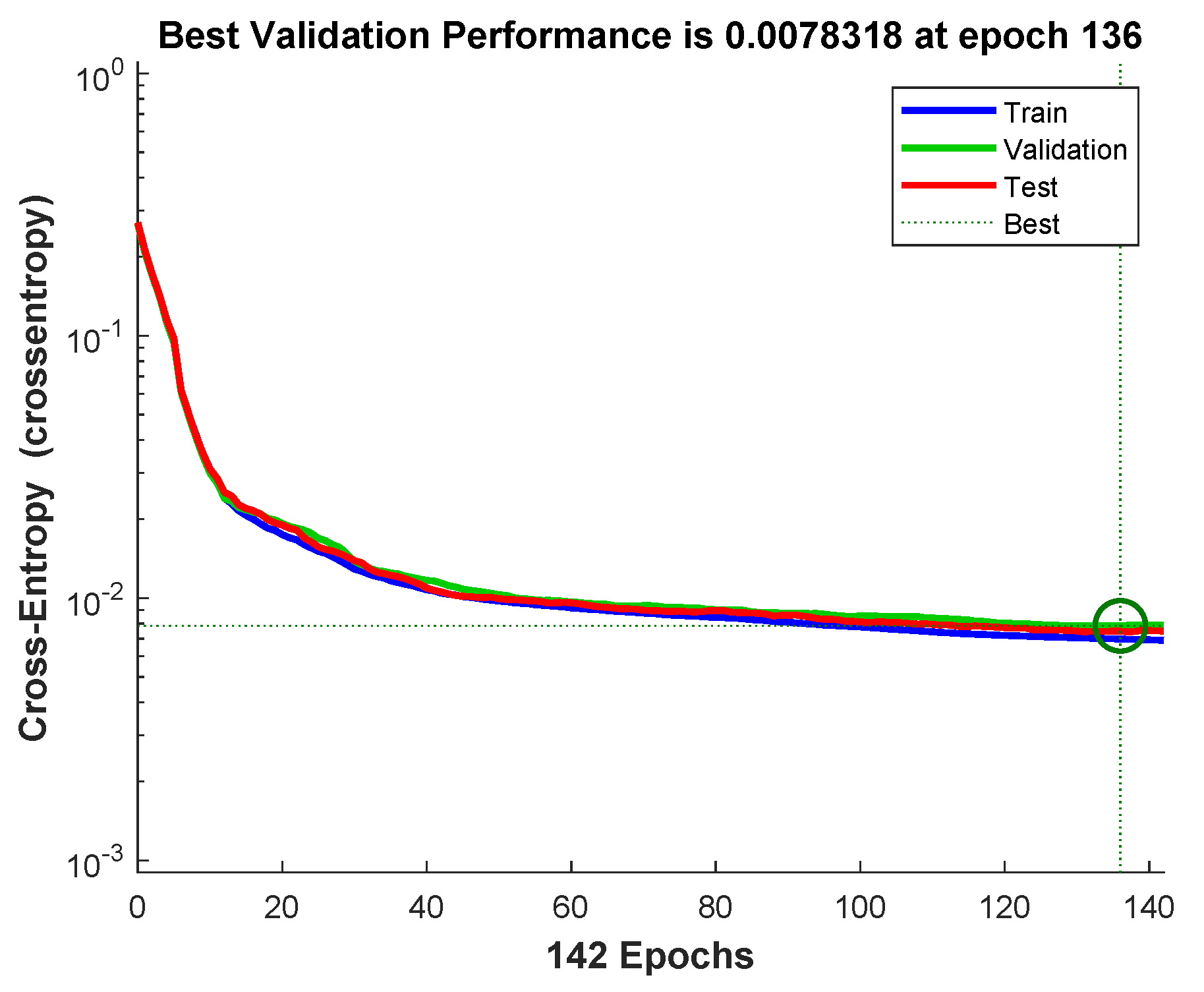
Lower the cross entropy higher the classification accuracy, zero cross entropy means no error.
Figure 11 shows that cross entropy reaches
at iteration 136.
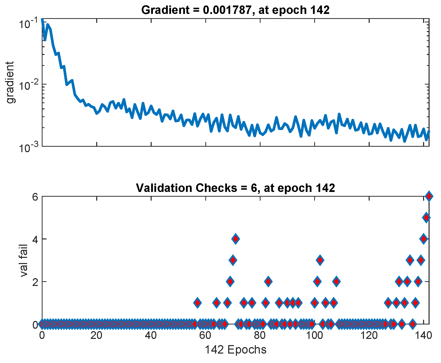
Figure 12 shows variation in gradient coefficient with respect to number of epochs. The final value of gradient coefficient at epoch number 142 is
which is approximately near to zero. Minimum the value of gradient coefficient better will be training and testing of networks. From the figure, it can be seen that the gradient value is decreasing with the increase in number of epochs. Large number of validation fails indicate the overtraining. In
Figure 12 validation fails are the iterations when validation mean square error (MSE) increased its value. A lot of fails means overtraining. MATLAB automatically stops training after 6 fails in a row.
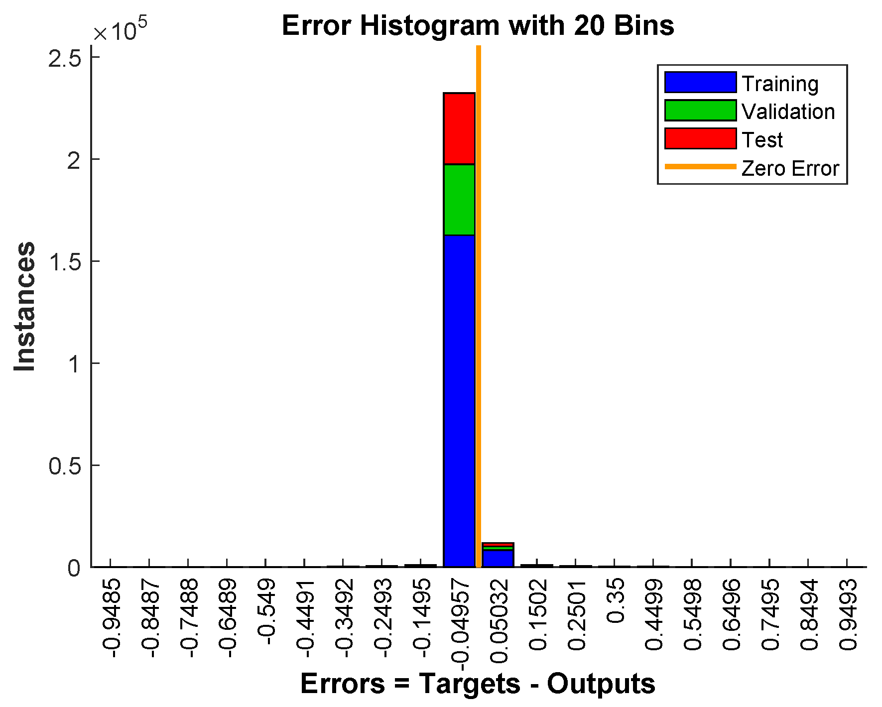
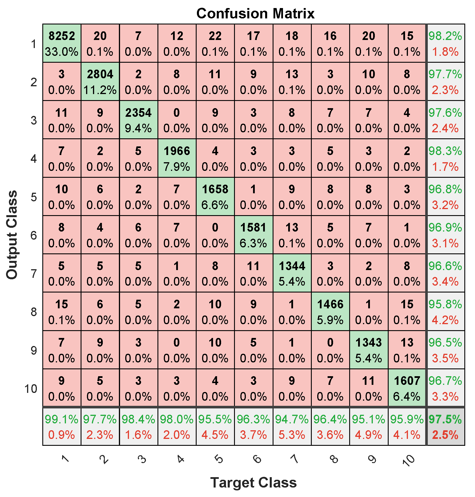
Figure 13 shows the error histogram of the trained neural network for the training, validation and testing parts. In this figure we can see that the data fitting errors are minimum and they are distributed within a closed range around zero. The confusion matrix
Figure 14 visualizes the performance of supervised learning. The rows correspond to the predicted user (Output Class) and the columns correspond to the true user (Target Class). The diagonal cells correspond to observations that are correctly assigned the user-RB pairs. The off-diagonal cells correspond to incorrectly assigned user-RB pairs. The trained neural network provides
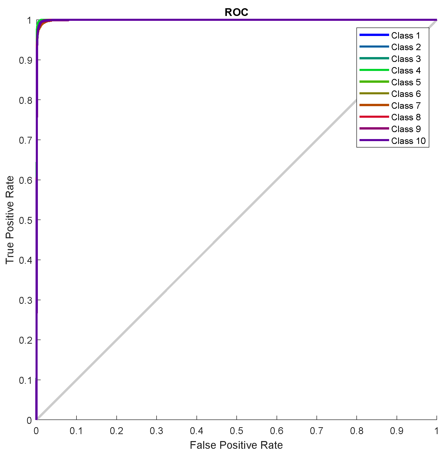
classification accuracy. The
Figure 15 represent the receiver operating characteristics (ROC) curves. The ROC curve plot shows the true positive rate versus the false positive rate as the threshold is varied. A perfect test would show points in the upper-left corner, with
sensitivity and
specificity [
28]. In the RB allocation module, it worked very well.
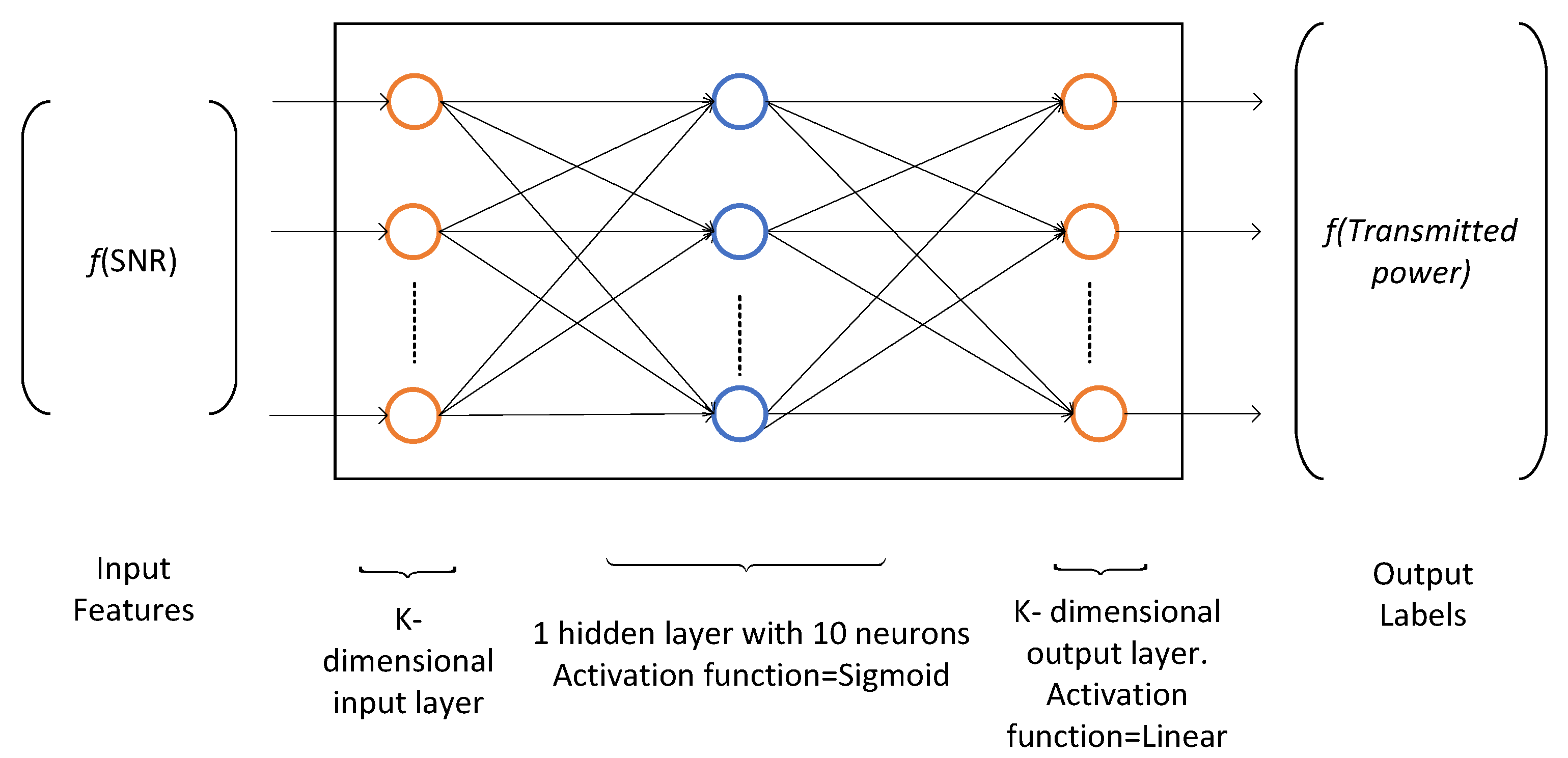
4.3. Power Allocation through Two-Layer Feedforward Neural Network
In the power allocation problem, we have to map the numeric input dataset (SNR) to the numeric output dataset (allocated power) per user per RB. Therefore, we use neural network curve fitting technique. The training dataset is generated by the Algorithm 2 as input received SNR and output allocated transmit power. Given the resource blocks allocation set
, the power allocation problem has been solved using two-layer feedforward neural network. The hidden layer neurons use sigmoid function as activation function and output neurons implement linear function as shown in
Figure 16. We use Bayesian Regularization method to train the neural network. This method typically requires more training time but gives good results for difficult and noisy dataset. The Bayesian Regularization method uses Levenberg-Marquardt optimization to update the weight and bias values. It minimizes a combination of squared errors and weights, and then determines the correct combination for better generalization. In this method, the training does not stops after six consecutive validation (improve) fails and by default max_fail = inf. The training continues until an optimal combination of errors and weights is reached. More detail on the use of Bayesian regularization, along with Levenberg-Marquardt training, can be found in [
29].
We use MATLAB 2019a App, Neural Net Fitting (nftool) which is a two-layer (one for hidden layer activation functions and other for output layer activation functions) feedforward network.
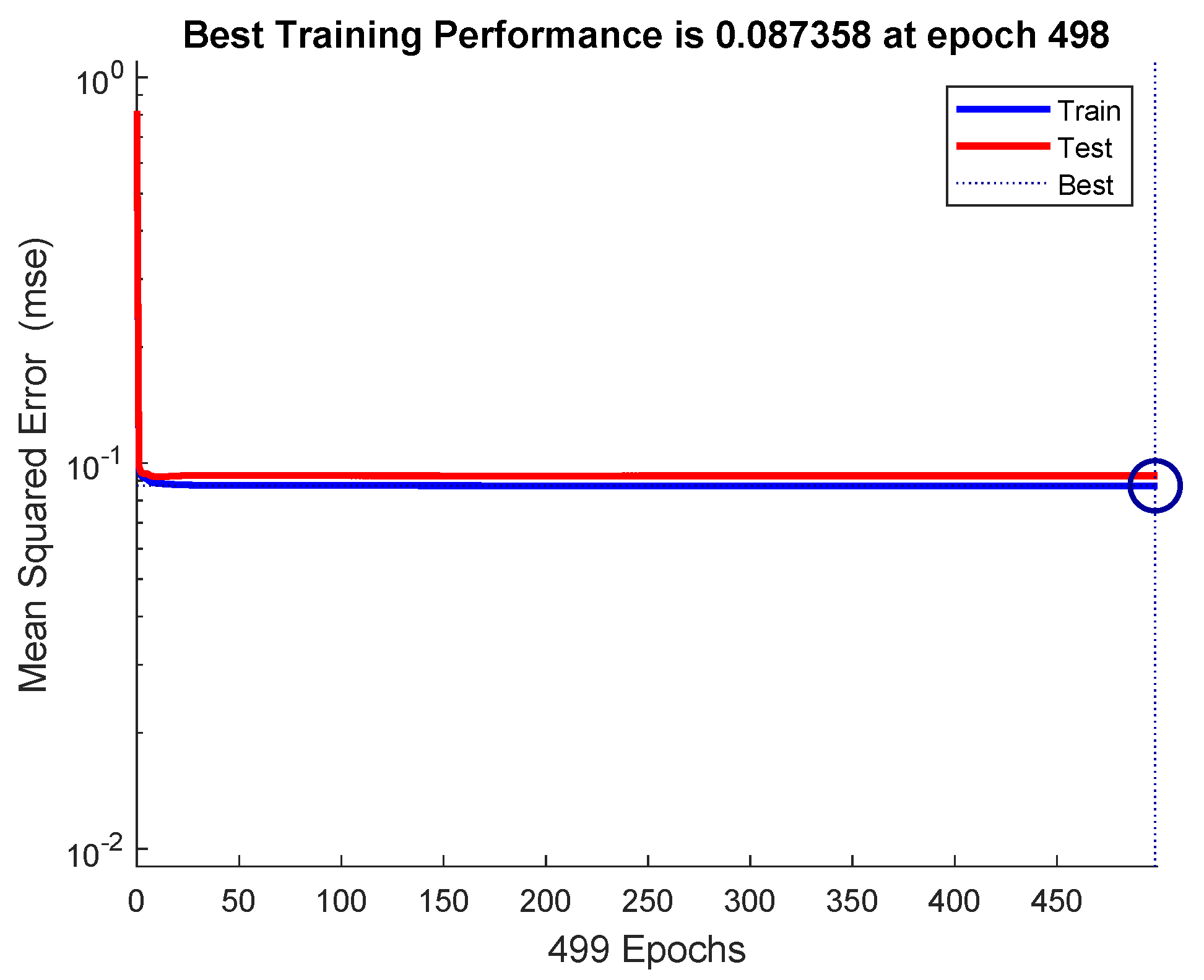
The mean-squared-error graph for the training and testing is shown in
Figure 17. It shows that the MSE reaches to
in 498 epochs. Our input/output samples to training network were channel gain/allocated power. Since, the total transmit power is a sum of linear functions of the channel gain, therefore, the neural network is got trained in a single epoch. An epoch is a full pass through the entire dataset and the calculation of new weights and biases.
Figure 18 shows that the gradient coefficient reaches to
in 499 epochs. The lower value of gradient ensures the training and testing of the network. Other parameters such as Mu, Num Parameters, and Sum Squared Param are the stop criteria defined in Bayesian regularization backpropagation function ’trainbr’ [
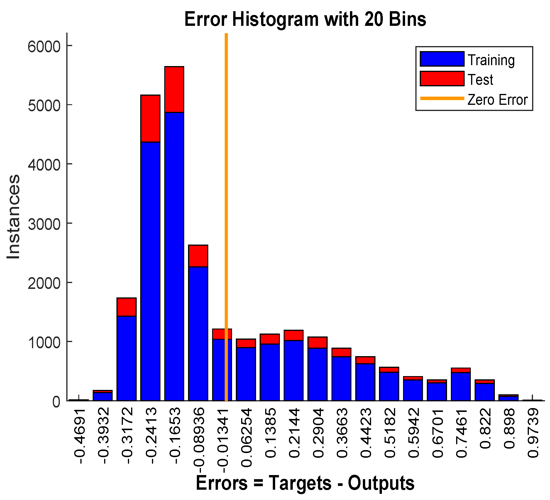
30]. Error histogram in
Figure 19 visualizes the errors between target values and the predicted values after training a feedforward neural network. In this figure we can see that the data fitting errors are minimum and they are distributed within a closed range around zero. Around
errors fall between
and
.
4.4. Performance Evaluation with Machine Learning Techniques
First, we apply the neural network for the RB and power allocation modules with a single relay. For the SAMM scheme in
Figure 20 shows
increase in the EE. This is because of the limitations of the BOPA method which sometimes returns no result, whereas, the neural network is trained on diverse dataset and always gives the output result. We also compare our proposed schemes with LERPA of [
11]. LERPA uses max–min criteria for RB allocation and fractional programming based transmission power control. In case of LTE network with multiple relays as shown in
Figure 7 or
Figure 9, the users associated with relay
q experience interference due to the neighboring relays
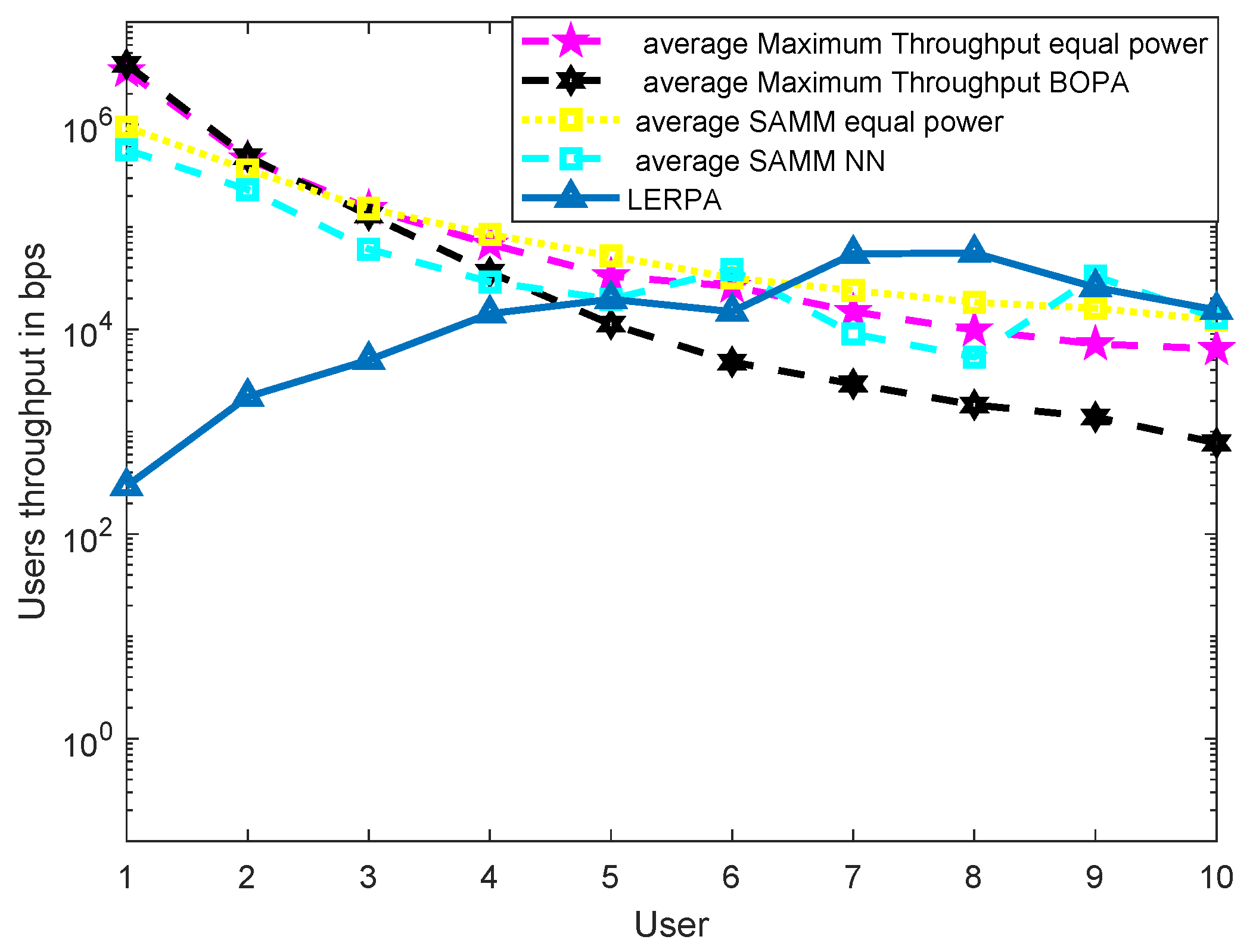
. This interference decreases the users’ throughput as shown in
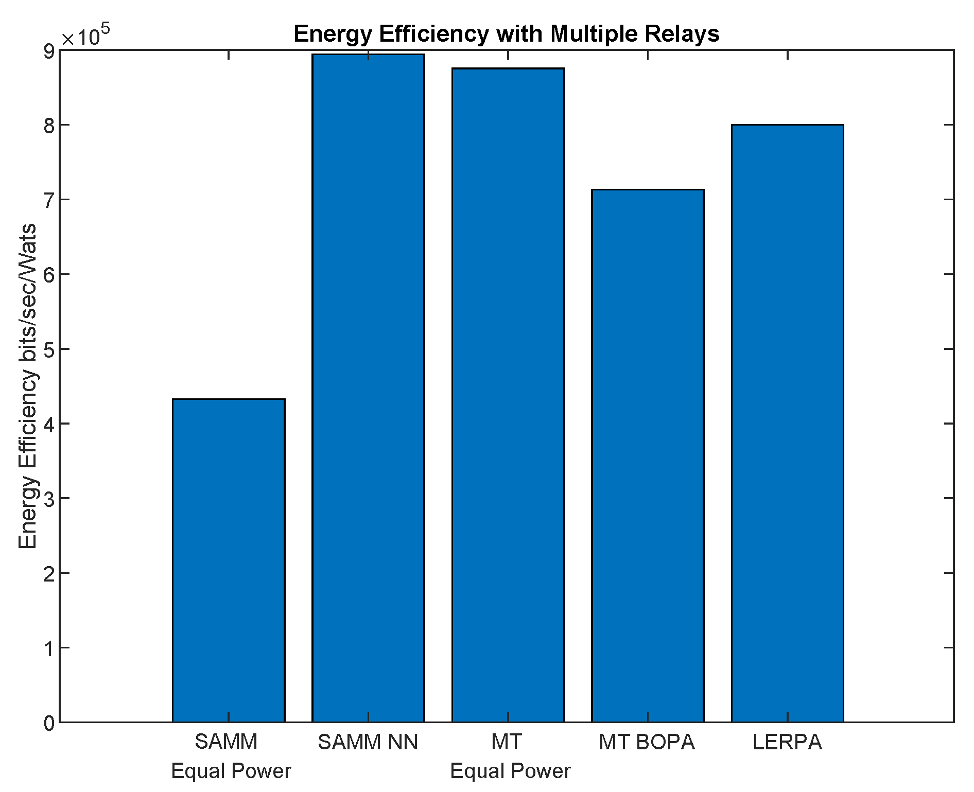
Figure 21. However, the EE maximization based NN power allocation continues to dominate in the multiple relay scenario. Since the transmission is orthogonal between BS and RNs, only the relay’s associated users are affected by the other relays transmissions. The equal power MT throughput does not affect because almost all the users are associated with BS. This further reduces the required transmit power of the relay, hence a net increase in EE has been observed in
Figure 22. Addition of multiple relays slightly affect the SAMM NN and SAMM equal power in positive and negative way, respectively. The PF component of the SAMM forces the association of low throughput users to increase the fairness. This association goes in positive way for the SAMM NN due to the EE based power allocation, but goes in negative way for the SAMM equal power because of no compensation of the interference power. The increased fairness of SAMM NN is evident from the
Figure 21, where, even the farthest users 9 and 10 have higher throughput. It can be seen that in LERPA, closer users get lower throughput but fairly large throughput is given to the farther users. This is because it uses max-min criterion for the RB allocation, which assigns the RB to the users who have lowest received SNR.
Table 3 summarizes simulation results.
It can be seen that SAMM with BOPA and NN compete well in fairness with best EE. Tradeoff has to be done on system throughput. LERPA has better fairness performance but is less efficient in EE and system throughput, whereas, the hypothetical MT performs better in average system throughput. We say hypothetical because it only allocates the RB and power to the users with the highest SNR which can not be applicable on practical scenarios.
5. Complexity Analysis
The RB allocation scheme SAMM uses alternate MT and PF metrics to assign the
N RBs to
K users. MT assigns
RBs to
K users and PF assigns
RBs to
users in alternate TTI. Therefore, the computational complexity of SAMM is
. The BOPA Algorithm 1, first requires
and
in line 4 using water-filling algorithm for which the worse-case complexity is
. After that, BOPA uses binary search method to estimate the roots of Equation (
17). In the worse case, with
points in the search space, binary search requires
iterations to find the roots of polynomial. In our case,
, where
is the error tolerance. Therefore, the overall complexity of the Algorithm 1 is
. In case of the optimal exhaustive search (
) RB allocation combining with the BOPA; the complexity is
, whereas, the complexity of SAMM-BOPA is
.
The running-time complexity of the K-mean algorithm is
[
31], where
k is the number of clusters,
m is the number of objects to be clustered,
d is the dimension of objects, and
i is the number of iterations. In our application of K-mean Algorithm 2, we use
and two-dimensional geographical location of the users. Therefore, the worse-case computational complexity is given as
.

 ,
, 


