
SAHARA: A Simplified AtmospHeric Correction AlgoRithm for Chinese gAofen Data: 1. Aerosol Algorithm

Abstract
:
1. Introduction
2. GaoFen-4 (GF4) Data
3. Method
3.1. Surface Parameterization
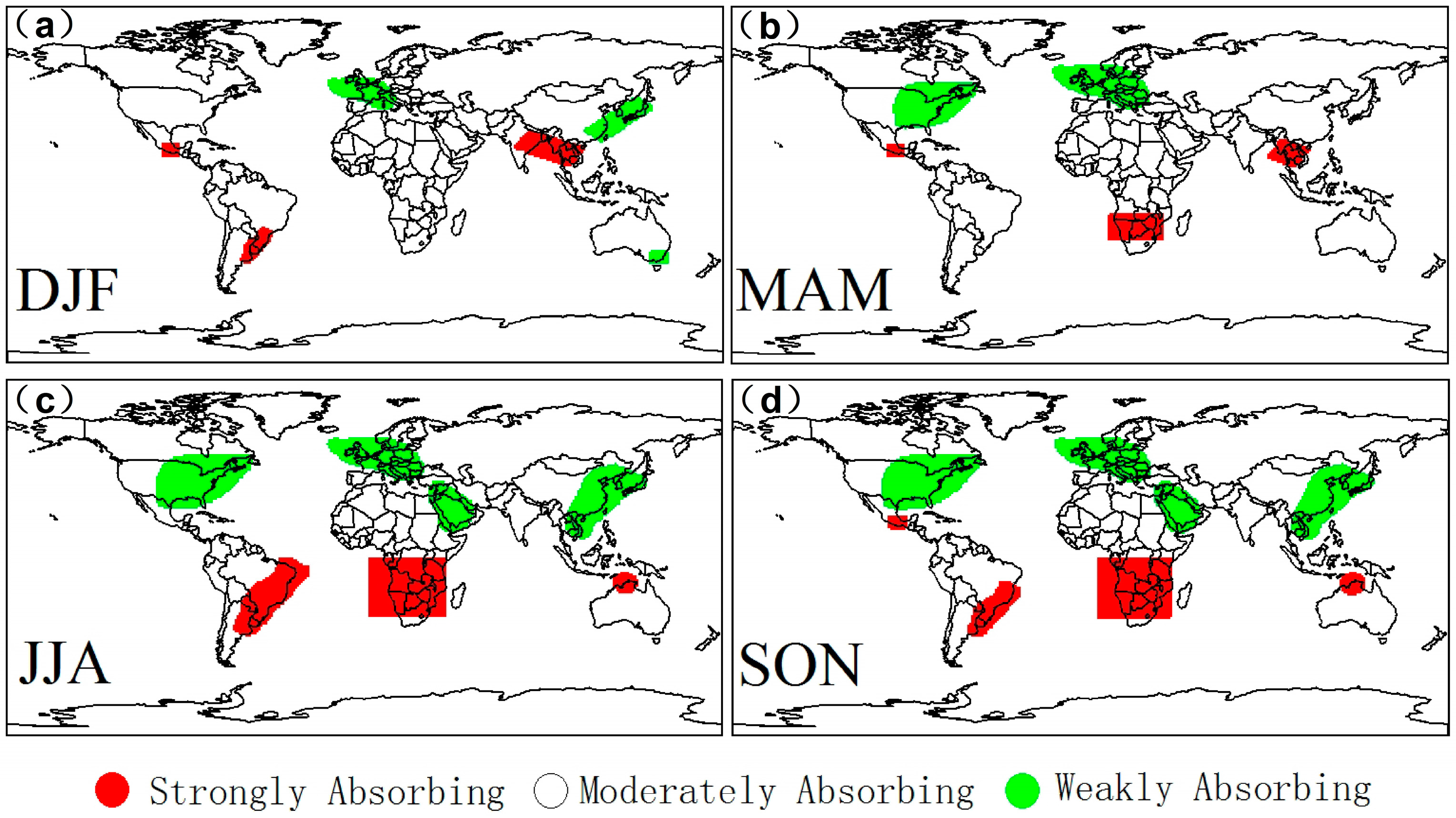
3.2. Aerosol Type Parameteirzation
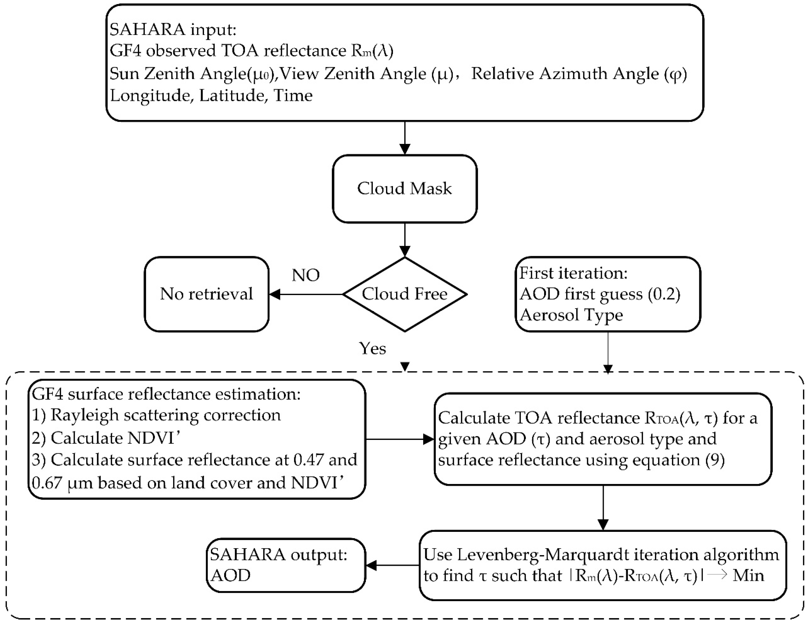
3.3. Aerosol Retrieval Algorithm
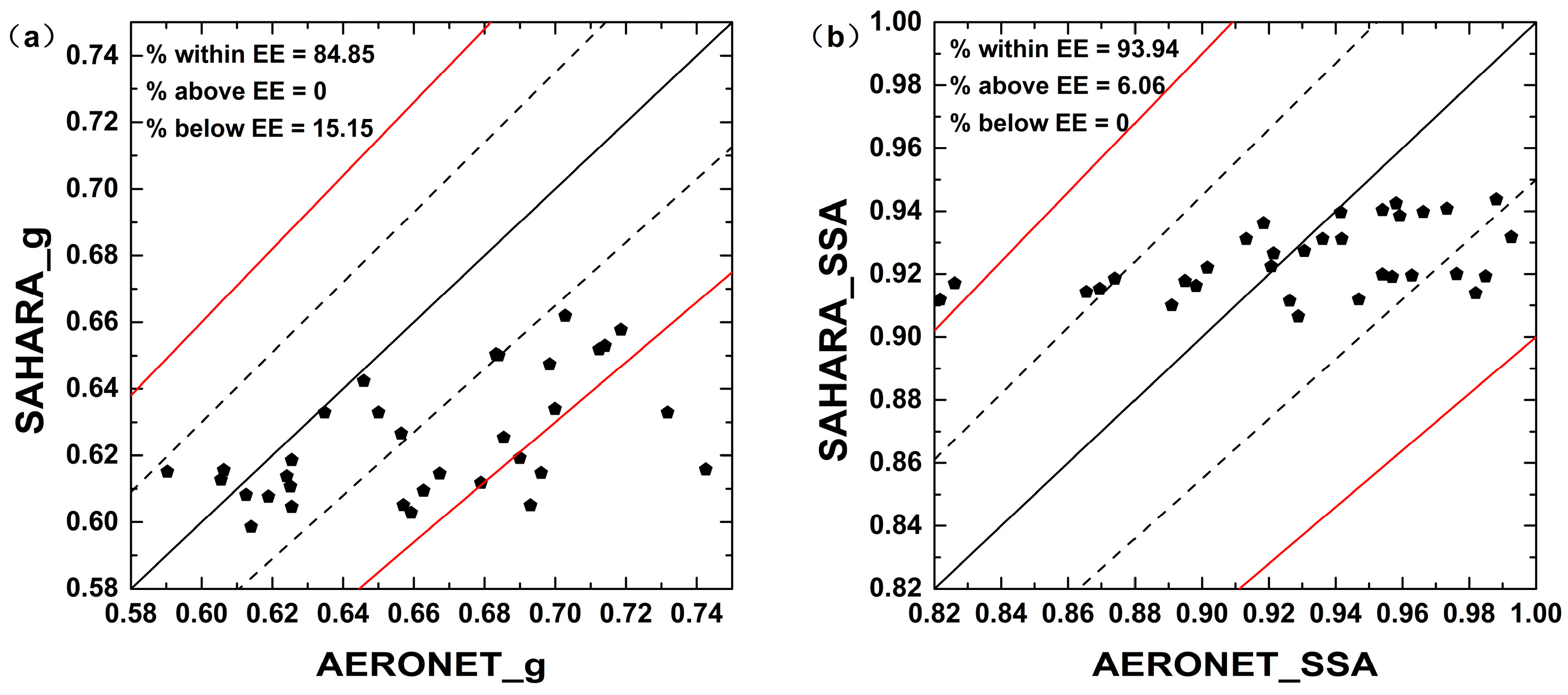
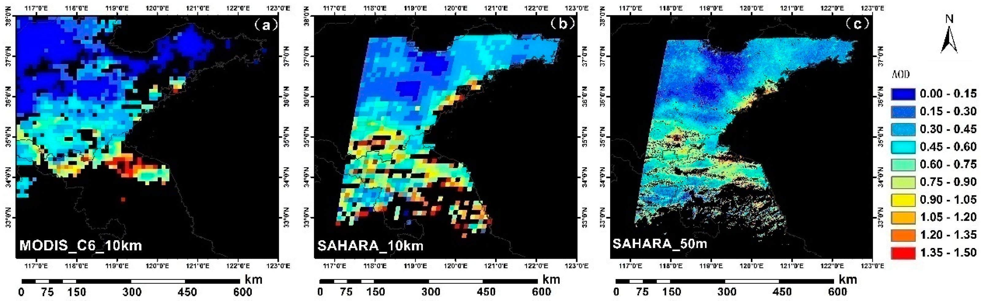
4. Results and Discussion
5. Conclusions
Acknowledgments
Author Contributions
Conflicts of Interest
Appendix A

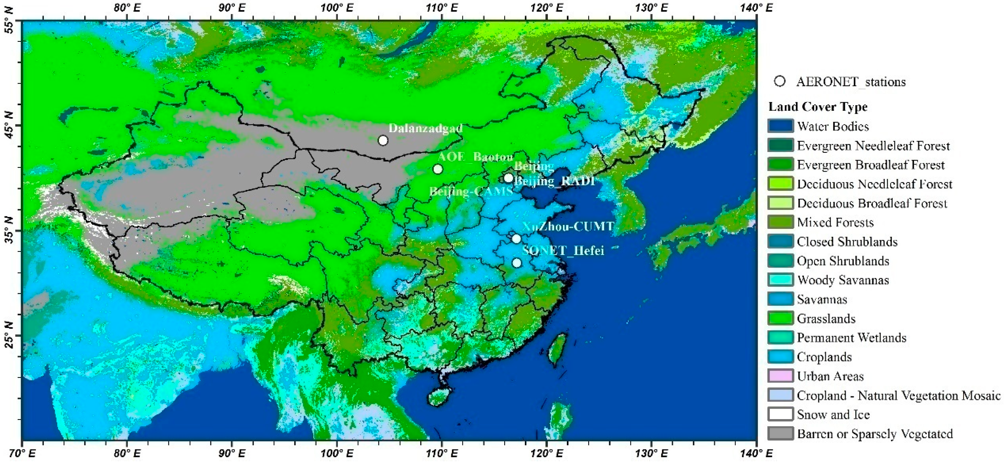
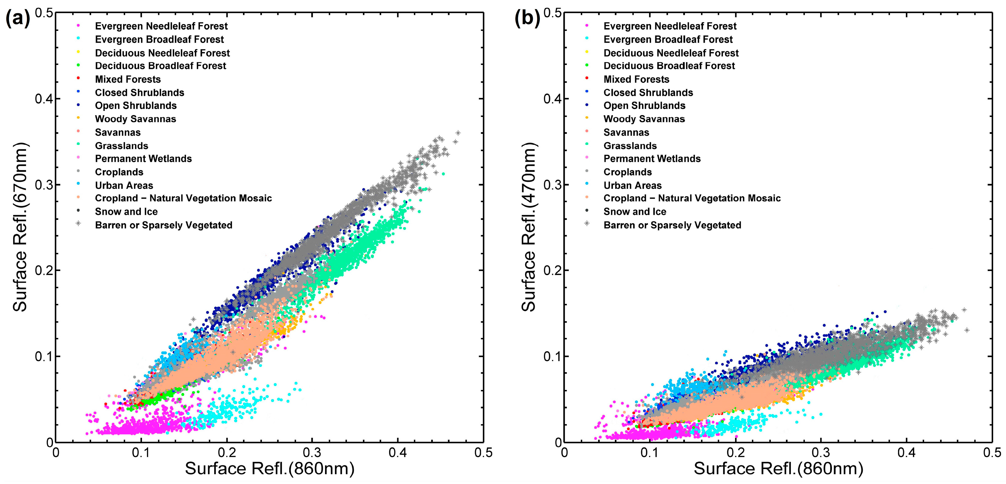
| No | Land Cover | No | Land Cover |
|---|---|---|---|
| 1 | Evergreen Needleleaf Forest | 9 | Savannas |
| 2 | Evergreen Broadleaf Forest | 10 | Grasslands |
| 3 | Deciduous Needleleaf Forest | 11 | Permanent Wetlands |
| 4 | Deciduous Broadleaf Forest | 12 | Croplands |
| 5 | Mixed Forests | 13 | Urban Areas |
| 6 | Closed Shrublands | 14 | Cropland - Natural Vegetation Mosaic |
| 7 | Open Shrublands | 15 | Snow and Ice |
| 8 | Woody Savannas | 16 | Barren or Sparsely Vegetated |
References
- Bassani, C.; Manzo, C.; Braga, F.; Bresciani, M.; Giardino, C.; Alberotanza, L. The impact of the microphysical properties of aerosol on the atmospheric correction of hyperspectral data in coastal waters. Atmos. Meas. Tech. 2015, 8, 1593–1604. [Google Scholar] [CrossRef]
- Tirelli, C.; Curci, G.; Manzo, C.; Tuccella, P.; Bassani, C. Effect of the Aerosol Model Assumption on the Atmospheric Correction over Land: Case Studies with CHRIS/PROBA Hyperspectral Images over Benelux. Remote Sens. 2015, 7, 8391–8415. [Google Scholar] [CrossRef] [Green Version]
- Koren, I.; Remer, L.R.; Kaufman, Y.J.; Rudich, Y.; Martins, J.V. On the twilight zone between clouds and aerosols. Geophys. Res. Lett. 2007, 34, L08805. [Google Scholar] [CrossRef]
- Mei, L.; Vountas, M.; Gomez-Chova, L.; Rozanov, V.; Jager, M.; Lotz, W.; Burrows, J.P.; Hollmann, R. A Cloud masking algorithm for the XBAER aerosol retrieval using MERIS data. Remote Sens. Environ. 2016. [Google Scholar] [CrossRef]
- Levy, R.C.; Mattoo, S.; Munchak, L.A.; Remer, L.A.; Sayer, A.M.; Patadia, F.; Hsu, N.C. The Collection 6 MODIS aerosol products over land and ocean. Atmos. Meas. Tech. 2013, 6, 2989–3034. [Google Scholar] [CrossRef]
- Hsu, N.C.; Jeong, M.J.; Bettenhausen, C.; Sayer, A.M.; Hansell, R.; Seftor, C.S.; Huang, J.; Tsay, S.C. Enhanced DB aerosol retrieval algorithm: The second generation. J. Geophys. Res. Atmos. 2013, 118, 9296–9315. [Google Scholar] [CrossRef]
- Bilal, M.; Nichol, J.E.; Bleiweiss, M.P.; Dubois, D. A Simplified high resolution MODIS Aerosol Retrieval Algorithm (SARA) for use over mixed surfaces. Remote Sens. Environ. 2013, 136, 135–145. [Google Scholar] [CrossRef]
- Mei, L.; Xue, Y.; de Leeuw, G.; Holzer-Popp, T.; Guang, J.; Li, Y.; Yang, L.; Xu, X.; Li, C.; Wang, Y.; et al. Retrieval of aerosol optical depth over land based on a time series technique using MSG/SEVIRI data. Atmos. Chem. Phys. 2012, 12, 9167–9185. [Google Scholar] [CrossRef]
- Lyapustin, A.; Wang, Y.; Laszlo, I.; Kahn, R.; Korkin, S.; Remer, L.; Levy, R.; Reid, J.S. Multiangle implementation of atmospheric correction (MAIAC): 2. Aerosol algorithm. J. Geophys. Res. Atmos. 2011, 116, D03211. [Google Scholar] [CrossRef]
- Katsev, I.L.; Prikhach, A.S.; Zege, E.P.; Ivanov, A.P.; Kokhanovsky, A.A. Iterative Procedure for Retrieval of Spectral Aerosol Optical Thickness and Surface Reflectance from Satellite Data Using Fast Radiative Transfer Code and Its Application to MERIS Measurements. In Satellite Aerosol Remote Sensing over Land, 1st ed.; Kokhanovsky, A.A., de Leeuw, G., Eds.; Praxis Publishing: Chichester, UK, 2009; pp. 101–134. [Google Scholar]
- Seidel, F.C.; Kokhanovsky, A.A.; Schaepman, M.E. Fast retrieval of aerosol optical depth and its sensitivity to surface albedo using remote sensing data. Atmos. Res. 2012, 116, 22–32. [Google Scholar] [CrossRef]
- Kaufman, Y.J.; Tanre, D.; Remer, L.A.; Vermote, E.F.; Chu, A.; Holben, B.N. Operational remote sensing of tropospheric aerosol over land from EOS moderate resolution imaging spectral radiometer. J. Geophys. Res. Atmos. 1997, 102, 17051–17067. [Google Scholar] [CrossRef]
- Chandrasekhar, S. Raditive Transfer, 1st ed.; Oxford University Press: New York, NY, USA, 1960; pp. 20–30. [Google Scholar]
- Eck, T.F.; Holben, B.N.; Slutsker, I.; Setzer, A. Measurements of irradiance attenuation and estimation of aerosol single scattering albedo for biomass burning aerosols in Amazonia. J. Geophys. Res. 1998, 103, 31865–31878. [Google Scholar] [CrossRef]
- Eck, T.F.; Holben, B.N.; Ward, D.E.; Dubovik, O.; Reid, J.S.; Smirnov, A.; Mukelabai, M.M.; Hsu, N.C.; O’ Neil, N.T.; Slutsker, I. Characterization of the optical properties of biomass burning aerosols in Zambia during the 1997 ZIBBEE field campaign. J. Geophys. Res. 2001, 106, 3425–3448. [Google Scholar] [CrossRef]
- Dubovik, O.; Holben, B.; Eck, T.F.; Smrnov, A.; Kaufman, Y.J.; King, M.D.; Tanre, D.; Slutsker, I. Variability of absorption and optical properties of key aerosol types observed in worldwide locations. J. Atmos. Sci. 2002, 59, 590–608. [Google Scholar] [CrossRef]
- Hansen, J.; Sato, M.; Ruedy, R. Radiative forcing and climate response. J. Geophys. Res. 1997, 102, 6831–6864. [Google Scholar] [CrossRef]
- Kambezidis, H.D.; Kaskaoutis, D.G. Aerosol climatology over four AERONET sites: An overview. Atmos. Environ. 2007, 8, 1892–1906. [Google Scholar] [CrossRef]
- Shettle, E.P.; Fenn, R.W. Models of Aerosols of Lower Troposphere and the Effect of Humidity Variations on Their Optical Properties; AFCRL Technical Report 790214; Air Force Cambridge Research Laboratory: Hanscom Air Force Base, MA, USA, 1979; p. 100. [Google Scholar]
- Keopke, P.; Hess, M.; Schult, I.; Shettle, E.P. Global Aerosol Data Set; MPI Meteorologie Hamburg Rep; Max-Planck-Institut für Meteorologie: Hamburg, Germany, 1997; p. 44. [Google Scholar]
- Munchak, L.A.; Levy, R.C.; Mattoo, S.; Remer, L.A.; Holben, B.N.; Schafer, J.S.; Hostetler, C.A.; Ferrare, R.A. MODIS 3 km aerosol product: Applications over land in an urban/suburban region. Atmos. Meas. Tech. 2013, 6, 1747–1759. [Google Scholar] [CrossRef]
- Remer, L.A.; Mattoo, S.; Levy, R.C.; Munchak, L.A. MODIS 3 km aerosol product: Algorithm and global perspective. Atmos. Meas. Tech. 2013, 6, 1829–1844. [Google Scholar] [CrossRef]
- Zhang, Y.; Li, Z.; Zhang, Y.; Hou, W.; Xu, H.; Chen, C.; Ma, Y. High temporal resolution aerosol retrieval using Geostationary Ocean Color Imager: Application and initial validation. J. Appl. Remote Sens. 2014, 8, 1435–1440. [Google Scholar] [CrossRef]
- Li, Y.; Xue, Y.; He, X.; Guang, J. High-resolution aerosol remote sensing retrieval over urban areas by synergetic use of HJ-1 CCD and MODIS data. Atmos. Environ. 2012, 46, 173–180. [Google Scholar] [CrossRef]
- Zhang, Y.; Liu, Z.; Wang, Y.; Ye, Z.; Leng, L. Inversion of Aerosol Optical Depth Based on the CCD and IRS Sensors on the HJ-1 Satellites. Remote Sens. 2014, 6, 8760–8778. [Google Scholar] [CrossRef]
- Vermote, E.; Justice, C.; Claverie, M.; Franch, B. Preliminary analysis of the performance of the Landsat 8/OLI land surface reflectance product. Remote Sens. Environ. 2016, 185, 45–56. [Google Scholar] [CrossRef]
- Luo, N.; Wong, M.; Zhao, W.; Yan, X.; Xiao, F. Improved aerosol retrieval algorithm using Landsat images and its application for PM10 monitoring over urban areas. Atmos. Res. 2015, 153, 264–275. [Google Scholar] [CrossRef]
- Sun, L.; Wei, J.; Bilal, M.; Tian, X.; Jia, C.; Guo, Y. Aerosol Optical Depth Retrieval over Bright Areas Using Landsat 8 OLI Images. Remote Sens. 2016, 8, 23. [Google Scholar] [CrossRef]
- Hagolle, O.; Huc, M.; Pascual, D.; Dedieu, G. A Multi-Temporal and Multi-Spectral Method to Estimate Aerosol Optical Thickness over Land, for the Atmospheric Correction of FormoSat-2, LandSat, VENμS and Sentinel-2 Images. Remote Sens. 2015, 7, 2668–2691. [Google Scholar] [CrossRef]
- Popp, T.; de Leeuw, G.; Bingen, C.; Bruhl, C.; Capelle, V.; Chedin, A.; Clarisse, L.; Dubovik, O.; Griesfeller, J.; Heckel, A.; et al. Development, production and evaluation of aerosol climate data records from European satellite observations (Aerosol_cci). Remote Sens. 2016, 8, 421. [Google Scholar] [CrossRef]
- Sinyuk, A.; Dubovik, O.; Holben, B.; Eck, T.F.; Breon, F.-M.; Martonchik, J.; Kahn, R.; Diner, D.J.; Vermote, E.F.; Roger, J.-C.; et al. Simultaneous retrieval of aerosol and surface properties from a combination of AERONET and satellite data. Remote Sens. 2007, 107, 90–108. [Google Scholar] [CrossRef]
- Wang, Z.; Li, X.; Li, S.; Chen, L. Quickly atmospheric correction for GF-1 WFV cameras. J. Remote Sens. 2016, 20, 353–360. [Google Scholar]
- Bao, F.; Gu, X.; Cheng, T.; Wang, Y.; Guo, H.; Chen, H.; Wei, X.; Xiang, K.; Li, Y. High-Spatial-Resolution Aerosol Optical Properties Retrieval Algorithm Using Chinese High-Resolution Earth Observation Satellite I. IEEE Trans. Geosci. Remote Sens. 2016, 54, 5544–5552. [Google Scholar] [CrossRef]
- Lawson, C.; Hanson, R. Solving Least Squares Problems; Prentice-Hall: Englewood Cliffs, NJ, USA, 1974. [Google Scholar]
- Tong, X.D. Development of China high-resolution earth observation system. J. Remote Sens. 2016, 20, 775–780. [Google Scholar]
- Friedl, M.A.; Mciver, D.K.; Hodges, J.C.F.; Zhang, X.Y.; Muchoney, D.; Strahler, A.H.; Woodcock, C.E.; Gopal, S.; Schneider, A.; Cooper, A. Global land cover mapping from modis: Algorithms and early results. Remote Sens. Environ. 2002, 83, 287–302. [Google Scholar] [CrossRef]
- Bassani, C.; Manzo, C.; Zakey, A.; Cuevas-Agulló, E. Effect of the Aerosol Type Selection for the Retrieval of Shortwave Ground Net Radiation: Case Study Using Landsat 8 Data. Atmosphere 2016, 7, 111. [Google Scholar] [CrossRef]
- Holzer-Popp, T.; Schroedter, M.; Gesell, G. Retrieving aerosol optical depth and type in the boundary layer over land and ocean from simultaneous GOME spectrometer and ATSR-2 radiometer measurements, 1, Method description. J. Geophys. Res. Atmos. 2002, 107. [Google Scholar] [CrossRef]
- Mei, L.; Xue, Y.; Kokhanovsky, A.A.; von Hoyningen-Huene, W.; de Leeuw, G.; Burrows, J.P. Retrieval of aerosol optical depth over land surfaces from AVHRR data. Atmos. Meas. Tech. 2014, 7, 2411–2420. [Google Scholar] [CrossRef] [Green Version]
- Mei, L.; Rozanov, V.; Vountas, M.; Burrows, J.P.; Levy, R.C.; Lotz, W. Retrieval of aerosol optical properties usingMERIS observations: Algorithm and some first results. Remote Sens. Environ. 2016. [Google Scholar] [CrossRef]
- Levy, R.C.; Remer, L.A.; Dubovik, O. Global aerosol optical properties and application to Moderate Resolution Imaging Spectroradiometer aerosol retrieval over land. J. Geophys. Res. Atmos. 2007, 112. [Google Scholar] [CrossRef]
- Wu, Y.; Graaf, M.; Menenti, M. Improved MODIS DT aerosol optical depth algorithm over land: Angular effect correction. Atmos. Meas. Tech. 2016, 9, 5575–5589. [Google Scholar] [CrossRef]
- Vermote, E.F.; Roger, J.C.; Ray, J.P. MODIS Surface Reflectance User’s Guide, Collection 6, 2015. Available online: http://modis-sr.ltdri.org/guide/MOD09_UserGuide_v1.4.pdf (accessed on 9 November 2016).
- Zhang, Q.; Xin, J.; Yan, Y.; Wang, L.L.; Wang, Y. The Variations and Trends of MODIS C5 & C6 Products’ Errors in the Recent Decade over the Background and Urban Areas of North China. Remote Sens. 2016, 8, 754. [Google Scholar]
- Holben, B.N.; Eck, T.F.; Slutsker, I.; Tanr´e, D.; Buis, J.P.; Setzer, A.; Vermote, E.; Reagan, J.A.; Kaufman, Y.J.; Nakajima, T.; et al. AERONET – A federated instrument network and data archive for aerosol characterization. Remote Sens. Environ. 1998, 66, 1–16. [Google Scholar] [CrossRef]
- Vermote, E.F.; Tanre, D.; Deuze, J.L.; Herman, M.; Morcrette, J. Second Simulation of the Satellite Signal in the Solar Spectrum, 6S: An overview. IEEE Trans. Geosci. Remote Sens. 1997, 35, 675–686. [Google Scholar] [CrossRef]
- Kokhanovsky, A.A.; Mayer, B.; Rozanov, V.V. A parameterization of the diffuse transmittance and reflectance for aerosol remote sensing problems. Atmos. Res. 2005, 73, 37–43. [Google Scholar] [CrossRef] [Green Version]
- Fröhlich, C.; Shaw, G.E. New determination of Rayleigh scattering in the terrestrial atmosphere. Appl. Opt. 1980, 19, 1773–1775. [Google Scholar] [CrossRef] [PubMed]
- Rahman, H.; Pinty, B.; Verstraete, M.M. Coupled surface-atmosphere reflectance (CSAR) model: 2. Semiempirical surface model usable with NOAA advanced very high resolution radiometer data. Geophys. Res. Atmos. 1993, 98, 20791–20801. [Google Scholar] [CrossRef]
- Xu, W.; Long, X.; Li, Q.; Cui, L.; Zhong, H. Image Radiometric and Geometric Accuracy Evaluation of GF-4 Satellite. Spacecr. Recovery Remote Sens. 2016, 4, 16–25. [Google Scholar]
- Che, H.; Zhang, X.-Y.; Xia, X.; Goloub, P.; Holben, B.; Zhao, H.; Wang, Y.; Zhang, X.-C.; Wang, H.; Blarel, L.; et al. Ground-based aerosol climatology of China: Aerosol optical depths from the China Aerosol Remote Sensing Network (CARSNET) 2002–2013. Atmos. Chem. Phys. 2015, 15, 7619–7652. [Google Scholar] [CrossRef]
- Wang, L.; Xin, J.; Wang, Y.; Li, Z.; Wang, P.; Liu, G.; Wen, T. Validation of MODIS aerosol products by CSHNET over China. Chin. Sci. Bull. 2007, 52, 1708–1718. [Google Scholar] [CrossRef]
- Seidel, F.C.; Kokhanovsky, A.A.; Schaepman, M.E. Fast and simple model for atmospheric radiative transfer. Atmos. Meas. Tech. 2010, 3, 1129–1141. [Google Scholar] [CrossRef] [Green Version]
- Von Hoyningen-Huene, W.; Yoon, J.; Vountas, M.; Istomina, L.G.; Rohen, G.; Dinter, T.; Kokhanovsky, A.A.; Burrows, J.P. Retrieval of spectral aerosol optical thickness over land using ocean color sensors MERIS and SeaWiFS. Atmos. Meas. Tech. 2011, 4, 151–171. [Google Scholar] [CrossRef] [Green Version]
- Mei, L.; Rozanov, V.; Vountas, M.; Burrows, J.P.; Richter, A. XBAER derived aerosol optical thickness from OLCI/Sentinel-3 observation. Atmos. Chem. Phys. 2017. (submitted). [Google Scholar]
- Liu, Z.; Liu, Q.; Lin, H.-C.; Schwartz, C.S.; Lee, Y.-H.; Wang, T. Three-dimensional variational assimilation of MODIS aerosol optical depth: Implementation and application to a dust storm over East Asia. J. Geophys. Res. 2011, 116, D23206. [Google Scholar] [CrossRef]
- Schwartz, C.S.; Liu, Z.; Lin, H.-C.; Cetola, J.D. Assimilating aerosol observations with a “hybrid” variational-ensemble data assimilation system. J. Geophys. Res. Atmos. 2014, 119, 4043–4069. [Google Scholar] [CrossRef]
- Roujean, J.L.; Leroy, M.; Deschamps, P.Y. A bidirectional reflectance model of the Earth’s surface for the correction of remote sensing data. J. Geophys. Res. 1992, 97, 20455–20468. [Google Scholar] [CrossRef]
- Schaaf, C.B.; Gao, F.; Strahler, A.H.; Lucht, W.; Li, X.; Tsang, T.; Strugnell, C.; Zhang, X.; Jin, Y.; Muller, J.; et al. First operational BRDF, albedo nadir reflectance products from MODIS. Remote Sens. Environ. 2003, 83, 135–148. [Google Scholar] [CrossRef]


| GF4 Band Number | GF4 Band-Width (µm) | Resolution (m) | MODIS Band Number | MODIS Band-Width (µm) | Resolution (m) |
|---|---|---|---|---|---|
| 1 | 0.45–0.9 | 50 m | |||
| 2 | 0.45–0.52 | 50 m | 4 | 0.459–0.479 | 500 m |
| 3 | 0.52–0.60 | 50 m | 3 | 0.545–0.565 | 500 m |
| 4 | 0.63–0.69 | 50 m | 1 | 0.620–0.670 | 250 m |
| 5 | 0.76–0.90 | 50 m | 2 | 0.841–0.876 | 250 m |
| 6 | 3.50–4.10 | 400 m |
| Land Cover | 0.10 < NDVI’ < 0.20 | 0.20 ≤ NDVI’ < 0.50 | 0.5 ≤ NDVI’ |
|---|---|---|---|
| 1 | 0.456, −2.450, −0.321, 1.730, −0.168 | −0.053, −0.743, −0.337, 1.329, 0.020 | −0.186, −0.358, −0.747, 1.912, 0.089 |
| 2 | −0.951, −1.494, −1.250, 3.953, 0.414 | 0.170, −1.195, 0.563, 0.085, −0.130 | 0.354, −0.414, 1.063, −1.610, −0.189 |
| 3 | |||
| 4 | |||
| 5 | −0.099, −1.886, 0.061, 1.358, −0.011 | 0.026, −0.432, 0.090, 0.181, −0.010 | 0.060, −0.499, 0.192, 0.065, −0.031 |
| 6 | 0.273, −1.445, 0.423, −0.499, −0.094 | ||
| 7 | −0.006, −0.890, −0.072, 0.562, 0.021 | 0.583, −0.762, 0.684, −1.429, −0.202 | |
| 8 | −0.596, −0.573, −0.793, 3.101, 0.201 | 0.100, −0.377, 0.281, −0.254, −0.045 | −0.010, −0.363, 0.022, 0.319, 0.003 |
| 9 | |||
| 10 | 0.029, −1.089, 0.059, 0.446, −0.013 | 0.028, −0.575, 0.091, 0.315, −0.017 | 0.012, −0.271, 0.052, 0.198, −0.007 |
| 11 | |||
| 12 | −0.115, −1.219, −0.062, 1.208, 0.010 | 0.006, −0.500, 0.066, 0.308, −0.005 | 0.005, −0.433, 0.083, 0.236, −0.004 |
| 13 | −0.046, −2.090, 0.001, 1.282, −0.013 | 0.113, −1.019, 0.152, 0.429, −0.050 | |
| 14 | −0.128, −1.445, 0.216, 1.163, −0.045 | −0.039, −0.592, −0.057, 0.636, 0.012 | |
| 15 | |||
| 16 | −0.015, −2.396, −0.037, 0.806, 0.014 | 0.080, −1.502, −0.397, 1.542, −0.015 |
| Land Cover | 0.10 < NDVI’ < 0.20 | 0.20 ≤ NDVI’ < 0.50 | 0.5 ≤ NDVI’ |
|---|---|---|---|
| 1 | −0.115, −0.546, −0.211, 1.023, 0.047 | ||
| 2 | 0.008, −1.519, 0.187, 0.679, −0.002 | 0.168, −0.678, 0.314, −0.091, −0.076 | |
| 3 | |||
| 4 | 0.167, −0.554, 0.522, −0.733, −0.075 | ||
| 5 | 0.094, −1.448, 0.268, 0.638, −0.067 | −0.028, −0.571, −0.024, 0.605, 0.010 | |
| 6 | |||
| 7 | 0.201, −1.350, 0.370, −0.433, −0.063 | ||
| 8 | 0.011, −1.650, 0.202, 1.010, −0.052 | −0.124, −0.789, −0.079, 0.963, 0.034 | |
| 9 | |||
| 10 | −0.071, −1.848, −0.123, 1.098, 0.023 | −0.039, −0.554, −0.054, 0.651, 0.013 | 0.021, −0.403, 0.058, 0.251, −0.009 |
| 11 | |||
| 12 | −0.260, −2.270, −0.232, 1.886, 0.096 | 0.226, −1.249, 0.444, −0.062, −0.109 | −0.189, −0.652, −0.296, 1.338, 0.073 |
| 13 | −0.104, −1.362, −0.200, 1.471, 0.037 | ||
| 14 | −0.563, −1.524, −0.674, 2.946, 0.205 | −0.618, −0.703, −0.789, 2.491, 0.262 | |
| 15 | |||
| 16 | 0.069, −1.567, 0.133, 0.270, −0.021 | −0.009, −0.466, −0.005, 0.403, 0.015 |
| Land Cover | 0.10 < NDVI’ < 0.20 | 0.20 ≤ NDVI’ < 0.50 | 0.5 ≤ NDVI’ |
|---|---|---|---|
| 1 | 0.362, −2.306, 1.662, −1.471, −0.244 | 0.009, −0.890, 0.106, 0.424, −0.004 | 0.001, −0.344, 0.032, 0.287, 0.000 |
| 2 | −0.095, −1.425, −0.025, 1.187, 0.025 | −0.004, −0.365, 0.009, 0.343, 0.002 | |
| 3 | |||
| 4 | −0.012, −0.439, −0.009, 0.455, 0.005 | −0.227, −0.466, −0.573, 1.775, 0.100 | |
| 5 | 0.010, −1.577, 0.291, 0.816, −0.066 | −0.012, −0.446, 0.007, 0.406, 0.006 | −0.011, −0.418, 0.001, 0.402, 0.006 |
| 6 | −0.041, −0.501, −0.151, 0.795, 0.021 | ||
| 7 | 0.028, −0.469, 0.051, 0.221, 0.005 | −0.061, −0.488, −0.124, 0.679, 0.041 | |
| 8 | −0.134, −2.022, 0.041, 1.201, 0.057 | 0.020, −1.193, 0.178, 0.609, −0.028 | −0.016, −0.404, −0.004, 0.394, 0.008 |
| 9 | |||
| 10 | 0.010, −0.934, −0.017, 0.505, 0.002 | −0.008, −0.595, 0.005, 0.470, 0.005 | −0.003, −0.368, 0.029, 0.287, 0.003 |
| 11 | −0.031, −2.031, 0.562, 0.527, −0.030 | 0.018, −0.993, 0.031, 0.565, −0.011 | |
| 12 | −0.048, −1.480, 0.044, 0.847, 0.003 | −0.021, −0.501, −0.013, 0.473, 0.011 | −0.029, −0.503, −0.026, 0.529, 0.012 |
| 13 | −0.046, −1.490, 0.044, 0.891, 0.011 | −0.269, −0.580, −0.692, 2.104, 0.122 | |
| 14 | −0.384, −1.422, 0.044, 1.144, 0.153 | −0.035, −0.550, −0.031, 0.591, 0.011 | −0.010, −0.422, 0.004, 0.380, 0.006 |
| 15 | |||
| 16 | 0.023, −1.344, 0.056, 0.413, 0.003 | −0.034, −0.364, −0.046, 0.444, 0.033 |
| Land Cover | 0.10 < NDVI’ < 0.20 | 0.20 ≤ NDVI’ < 0.50 | 0.5 ≤ NDVI’ |
|---|---|---|---|
| 1 | −0.125, −1.788, −0.217, 1.542, 0.045 | 0.010, −0.959, 0.145, 0.448, −0.010 | 0.010, −0.365, 0.049, 0.258, −0.004 |
| 2 | 0.068, −0.847, 0.225, 0.237, −0.040 | 0.008, −0.334, 0.033, 0.265, −0.004 | |
| 3 | |||
| 4 | 0.047, −0.550, 0.254, 0.010, −0.027 | ||
| 5 | −0.003, −2.118, 0.407, 0.434, −0.026 | −0.004, −0.760, 0.077, 0.563, −0.008 | −0.009, −0.386, 0.007, 0.349, 0.006 |
| 6 | −0.015, −0.557, 0.013, 0.438, 0.009 | ||
| 7 | 0.059, −0.874, 0.114, 0.200, −0.015 | −0.040, −0.610, −0.029, 0.427, 0.044 | |
| 8 | −0.104, −1.499, 0.081, 1.068, 0.018 | −0.003, −0.619, 0.027, 0.453, 0.000 | 0.004, −0.382, 0.033, 0.294, −0.001 |
| 9 | |||
| 10 | 0.004, −0.836, 0.090, 0.420, −0.007 | −0.014, −0.560, 0.014, 0.471, 0.006 | 0.018, −0.317, 0.087, 0.132, −0.007 |
| 11 | −0.061, −2.128, −0.019, 1.184, 0.010 | −0.074, −0.696, −0.097, 0.768, 0.036 | |
| 12 | −0.108, −2.426, 0.059, 1.090, 0.025 | 0.011, −0.609, 0.094, 0.311, −0.006 | −0.009, −0.365, 0.015, 0.353, 0.002 |
| 13 | −0.071, −2.326, −0.018, 1.125, 0.023 | −0.037, −0.941, 0.013, 0.694, 0.015 | −0.012, −0.432, 0.001, 0.427, 0.005 |
| 14 | −0.018, −0.572, −0.005, 0.508, 0.007 | −0.007, −0.425, 0.003, 0.406, 0.002 | |
| 15 | |||
| 16 | −0.079, −0.365, −0.134, 0.603, 0.063 |
| Land Cover | 0.10 < NDVI’ < 0.20 | 0.20 ≤ NDVI’ < 0.50 | 0.5 ≤ NDVI’ |
|---|---|---|---|
| 1 | 0.0036, −1.657, −0.116, 1.353, 0.010 | 0.027, −1.551, −0.033 1.124, 0.003 | 0.063, −0.542, 0.196, 0.049, −0.0088 |
| 2 | −0.159, −3.625, −0.121, 1.765, −0.079 | −0.251, −0.69, −0.443, 1.617, 0.129 | −0.019, −0.661, −0.127, 0.902, 0.028 |
| 3 | |||
| 4 | −0.281, −1.230, −0.302, 1.791, 0.113 | ||
| 5 | −0.081, −1.512, −0.196, 1.496, 0.044 | −0.161, −1.071, −0.336, 1.679, 0.082 | −0.066, −0.631, −0.205, 1.033, 0.049 |
| 6 | 0.1435, −4.187, 0.358, 0.624, −0.055 | ||
| 7 | 0.0289, −1.909, −0.046, 1.294, −0.005 | −0.081, −0.788, −0.236, 1.550, 0.035 | |
| 8 | −0.0364, −1.963, −0.151,1.500, 0.027 | −0.257, −1.287, −0.467, 2.030, 0.123 | −0.123, −0.544, −0.351, 1.215, 0.080 |
| 9 | |||
| 10 | 0.0217, −1.2854, 0.069, 0.934, −0.008 | −0.0002, −1.075, −0.0536, 1.136, 0.005 | −0.043, −0.708, −0.217, 1.111, 0.038 |
| 11 | |||
| 12 | −0.0228, −2.366, −0.083, 1.399, 0.020 | −0.091, −1.244, −0.234, 1.529, 0.049 | −0.080, −0.662, −0.218, 1.151, 0.046 |
| 13 | −0.124, −0.240, −0.329, 1.571, 0.067 | −0.0525, −1.233, −0.216, 1.456, 0.034 | |
| 14 | 0.008, −2.698, −0.0189, 1.466, −0.013 | −0.172, −0.976, −0.392, 1.793, 0.082 | −0.0115, −0.60, −0.119, 0.831, 0.023 |
| 15 | −0.0645, −1.530, −0.191, 1.563, 0.037 | 0.051, −1.400, −0.0214, 1.058, −0.006 | 0.032, −0.520, 0.065, 0.435, −0.002 |
| 16 | 0.020, −1.657, −0.116, 1.353, 0.010 | −0.001, −1.349, −0.084, 1.234, 0.0136 | 0.059, −0.846, −0.041, 0.841, −0.009 |
| Land Cover | 0.10 < NDVI’ < 0.20 | 0.20 ≤ NDVI’ < 0.50 | 0.5 ≤ NDVI’ |
|---|---|---|---|
| 1 | −0.027, −0.378, −0.371, 1.141, 0.037 | 0.032, −0.553, 0.006, 0.442, 0.007 | |
| 2 | 0.061, −1.330, 0.024, 1.023, −0.024 | −0.063, −0.545, −0.196, 0.910, 0.050 | |
| 3 | |||
| 4 | −0.242, −0.459, −0.425, 1.405, 0.121 | ||
| 5 | 0.091, −1.237, 0.061, 0.956, −0.049 | −0.051, −0.409, −0.130, 0.644, 0.041 | |
| 6 | 0.144, −0.737, 0.254, 0.055, −0.049 | ||
| 7 | −0.077, −1.976, −0.189, 1.725, 0.033 | −0.029, −1.351, −0.143, 1.362,0.026 | |
| 8 | −0.041, −1.451, −0.151, 1.480,0.013 | −0.120, −0.404, −0.268, 0.954, 0.071 | |
| 9 | |||
| 10 | 0.0494, −1.524, 0.017, 1.076, −0.013 | 0.011, −1.344, −0.060, 1.161, 0.008 | −0.033, −0.636, −0.131, 0.870, 0.034 |
| 11 | 0.155, −1.337, 0.464, 0.114, −0.075 | −0.112, −0.600, −0.067, 0.668, 0.064 | |
| 12 | −0.359, −2.430, −0.441, 2.403, 0.145 | 0.135, −0.974, 0.230, 0.257, −0.044 | −0.013, −0.647, −0.080, 0.734, 0.025 |
| 13 | 0.016, −1.118, −0.070, 1.015, 0.010 | −0.056, −0.687, −0.151, 0.952, 0.043 | |
| 14 | 0.045, −1.479, 0.009, 1.018, −0.008 | −0.096, −0.490, −0.207, 0.865, 0.064 | |
| 15 | |||
| 16 | 0.027, −1.585, −0.032, 1.197, −0.002 | 0.005, −1.434, −0.083, 1.254, 0.011 | 0.102, −0.859, 0.086, 0.586, −0.028 |
| Land Cover | 0.10 < NDVI’ < 0.20 | 0.20 ≤ NDVI’ < 0.50 | 0.5 ≤ NDVI’ |
|---|---|---|---|
| 1 | 0.156, −2.234, 0.369, 0.429, −0.078 | 0.003, −0.860, −0.115, 0.963, 0.014 | 0.009, −0.433, −0.182, 0.794, 0.018 |
| 2 | −0.0622, −1.245, −0.149, 1.378, 0.021 | −0.032, −0.419, −0.128, 0.636, 0.040 | |
| 3 | |||
| 4 | −0.098, −0.616, −0.366, 1.450, 0.056 | −0.039, −0.654, −0.248, 1.105, 0.038 | |
| 5 | 0.005, −1.455, 0.147, 1.089, −0.044 | −0.032, −0.770, −0.1545, 0.964, 0.032 | 0.017, −0.387, −0.064, 0.472, 0.015 |
| 6 | −0.783, −2.326, −1.77, 5.309, 0.337 | −0.028, −0.393, −0.202, 0.988, 0.027 | −0.016, −0.901, −0.043, 0.969, 0.023 |
| 7 | −0.062, −0.483, −0.128, 1.147, 0.039 | −0.123, −1.233, −0.315, 1.657, 0.074 | |
| 8 | 0.176, −2.467, 0.321, 0.798, 0.111 | 0.011, −1.164, 0.003, 0.902, 0.001 | −0.023, −0.406, −0.123, 0.613, 0.035 |
| 9 | |||
| 10 | −0.017, −0.990, −0.056, 1.095, 0.016 | −0.055, −1.310, −0.188, 1.357, 0.044 | −0.016, −0.678, −0.164, 0.963, 0.028 |
| 11 | −0.039, −2.334, −0.408, 1.666, 0.0467 | 0.007, −0.968, −0.113, 1.117, 0.005 | 0.034, −0.778, −0.036, 0.825, −0.009 |
| 12 | −0.008, −0.926, −0.058, 1.081, −0.002 | −0.006, −0.901, −0.071, 0.925, 0.019 | −0.018, −0.589, −0.126, 0.785, 0.031 |
| 13 | −0.069, −1.395, −0.284, 1.565, 0.043 | 0.000, −1.036, −0.090, 0.948, 0.022 | −0.048, −0.526, −0.195, 0.863, 0.050 |
| 14 | −0.593, −2.030, −0.592, 2.400, 0.309 | −0.073, −0.578, −0.237, 1.081, 0.054 | −0.012, −0.575, −0.097, 0.707, 0.029 |
| 15 | |||
| 16 | −0.023, −0.928, −0.100, 1.195, 0.021 | −0.045, −1.246, −0.146, 1.301, 0.038 |
| Land Cover | 0.10 < NDVI’ < 0.20 | 0.20 ≤ NDVI’ < 0.50 | 0.5 ≤ NDVI’ |
|---|---|---|---|
| 1 | −0.114, −0.704, −0.167, 1.165, 0.083 | −0.091, −1.735, −0.198, 1.412, 0.073 | −0.086, −0.486, −0.338, 1.188, 0.057 |
| 2 | −0.387, −0.532, −1.176, 3.248, 0.180 | ||
| 3 | 0.080, −2.328, 0.056, 1.233, −0.04 | ||
| 4 | −0.074, −1.169, −0.192, 1.238, 0.049 | −0.377, −0.622, −1.24, 3.304, 0.188 | |
| 5 | 0.118, −1.00, 0.138, 0.779, −0.064 | −0.082, −1.513, −0.140, 1.386, 0.050 | −0.094, −0.513, −0.264, 0.989, 0.065 |
| 6 | |||
| 7 | 0.084, 0.511, −0.483, 1.49, 0.070 | −0.196, −1.523, −0.562, 2.072, 0.125 | −0.071, −0.522, −0.234, 0.911, 0.060 |
| 8 | −0.388, −1.127, −0.479, 1.937, 0.203 | −0.018, −2.23, 0.011, 1.037, 0.047 | −0.070, −0.390, −0.296, 1.008, 0.050 |
| 9 | |||
| 10 | −0.011, −0.703, −0.058, 1.071, 0.014 | −0.057, −1.501, −0.1256, 1.337, 0.036 | −0.033, −0.518, −0.157, 0.780, 0.037 |
| 11 | |||
| 12 | −0.027, −1.456, −0.111, 1.323, 0.017 | −0.036, −1.222, −0.193, 1.254, 0.032 | −0.090, −0.446, −0.321, 1.065, 0.061 |
| 13 | |||
| 14 | 0.056, −1.074, 0.348, 0.509, −0.034 | −0.021, −1.902, −0.075, 1.311, 0.026 | 0.186, −0.376, 0.148, 0.005, −0.066 |
| 15 | −0.078, −3.385, −0.034, 1.416, 0.048 | 0.043, −1.000, −0.114, 1.096, −0.013 | −0.009, −0.465, −0.103, 0.597, 0.027 |
| 16 | −0.070, −0.736, −0.139, 1.291, .0326 | −0.041, −1.349, −0.149, 1.311, 0.030 | 0.018, −0.544, −0.079, 0.655, 0.009 |
| SSA | a0 | a1 | a2 |
|---|---|---|---|
| Weakly absorbing | 0.921 | 0.049 | −0.018 |
| Moderately absorbing | 0.899 | 0.048 | −0.012 |
| Strongly absorbing | 0.831 | 0.044 | −0.018 |
| Alpha | a0 | a1 | a2 |
|---|---|---|---|
| Weakly absorbing | 1.926 | −0.217 | −0.162 |
| Moderately absorbing | 1.865 | 0.052 | −0.268 |
| Strongly absorbing | 2.028 | 0.008 | −0.096 |
| g | a0 | a1 | a2 |
|---|---|---|---|
| Weakly absorbing | 0.607 | 0.081 | −0.014 |
| Moderately absorbing | 0.59 | 0.053 | −0.003 |
| Strongly absorbing | 0.548 | −0.003 | 0.024 |
© 2017 by the authors. Licensee MDPI, Basel, Switzerland. This article is an open access article distributed under the terms and conditions of the Creative Commons Attribution (CC BY) license ( http://creativecommons.org/licenses/by/4.0/).
Share and Cite
She, L.; Mei, L.; Xue, Y.; Che, Y.; Guang, J. SAHARA: A Simplified AtmospHeric Correction AlgoRithm for Chinese gAofen Data: 1. Aerosol Algorithm. Remote Sens. 2017, 9, 253. https://doi.org/10.3390/rs9030253
She L, Mei L, Xue Y, Che Y, Guang J. SAHARA: A Simplified AtmospHeric Correction AlgoRithm for Chinese gAofen Data: 1. Aerosol Algorithm. Remote Sensing. 2017; 9(3):253. https://doi.org/10.3390/rs9030253
Chicago/Turabian StyleShe, Lu, Linlu Mei, Yong Xue, Yahui Che, and Jie Guang. 2017. "SAHARA: A Simplified AtmospHeric Correction AlgoRithm for Chinese gAofen Data: 1. Aerosol Algorithm" Remote Sensing 9, no. 3: 253. https://doi.org/10.3390/rs9030253