Article

Increasing Outbreak of Cyanobacterial Blooms in Large Lakes and Reservoirs under Pressures from Climate Change and Anthropogenic Interferences in the Middle–Lower Yangtze River Basin

1
Ministry of Education Key Laboratory for Biodiversity Science and Ecological Engineering, Coastal Ecosystems Research Station of the Yangtze River Estuary, and Shanghai Institute of EcoChongming (SIEC), Fudan University, Shanghai 200433, China
2
Department of Microbiology and Plant Biology, Center for Spatial Analysis, University of Oklahoma, Norman, OK 73019, USA
*
Author to whom correspondence should be addressed.
Remote Sens. 2019, 11(15), 1754; https://doi.org/10.3390/rs11151754
Submission received: 26 June 2019 / Revised: 20 July 2019 / Accepted: 22 July 2019 / Published: 25 July 2019

Abstract

:
In recent decades, the increasing frequency and severity of cyanobacterial blooms in recreational lakes and water supply reservoirs have become a great concern to public health and a significant threat to the environment. Cyanobacterial bloom monitoring is the basis of early warning and treatment. Previous research efforts have always focused on monitoring blooms in a few specific lakes in China using moderate resolution imaging spectroradiometer (MODIS) images, which are available for the years 2000 onward. However, the lack of overall information on long-term cyanobacterial blooms in the lakes and reservoirs in the middle–lower Yangtze River (MLYR) basin is an obstacle to better understanding the dynamics of cyanobacterial blooms at a watershed scale. In this study, we extracted the yearly coverage area and frequency of cyanobacterial blooms that occurred from 1990 to 2016 in 30 large lakes and 10 reservoirs (inundation area >50 km2) by using time series Landsat satellite images from Google Earth Engine (GEE). Then, we calculated the cyanobacterial bloom area percentage (CAP) and the cyanobacterial bloom frequency index (CFI) and analyzed their inter-annual variation and trends. We also investigated the main driving forces of changes in the CAP and CFI in each lake and reservoir. We found that all reservoirs and more than 60% of lakes exhibited an increasing frequency and coverage area of cyanobacterial blooms under the pressures of climate change and anthropogenic interferences. Reservoirs were more prone to be affected by fertilizer consumption from their regional surroundings than lakes. High temperatures increased blooms of cyanobacteria, while precipitation in the lake and reservoir regions somewhat alleviated blooms. This study completes the data records of cyanobacterial blooms in large lakes and reservoirs located in hotspots of the MLYR basin and provides more baseline information before 2000, which will present references for water resource management and freshwater conservation.

1. Introduction

Lakes, ponds, and reservoirs are major components of surface freshwater, which provide valuable ecosystem services, including drinking water supply, agricultural irrigation, fisheries, flood control, the hydrological cycle, and cultural services, amongst other services [1,2,3]. The adjacent regions of freshwater bodies are always accompanied by a high human population density, which results in activities that increase anthropogenic eutrophication and even large-scale cyanobacterial blooms [4]. Cyanobacterial bloom is a threat to public health as well as the ecosystem. As a consequence of climate change and anthropogenic activities, the severity and intensity of cyanobacterial blooms occurring in lakes, reservoirs, rivers, and marine ecosystems have been increasing in recent decades [5,6,7,8,9,10,11]. However, more data on the mechanisms of cyanobacterial blooms, especially long-term records are still required to complete our understanding of this phenomenon, which would allow for a more accurate assessment of the processes that drive these blooms [7,11].
The middle–lower Yangtze River (MLYR) basin, one of the most concentrated distributions of freshwater in East Asia, or even the world, serves as the water supply for a population size of nearly half a billion. It plays an essential role in maintaining regional ecological and environmental functions, as well as sustaining agricultural production and socioeconomic development [3,12,13,14]. Around 2000, many national construction projects related to afforestation and dams were carried out in this region, such as the construction of forest protection in the middle–lower Yangtze River starting in 2000, and the operation of the Three Gorges Dam starting in 2003, which significantly influenced the adjacent ecological environment [15,16,17]. As a result of the increase in anthropogenic activities over the past decades, most of the large lakes and reservoirs are now mesotrophic and even eutrophic in the MLYR basin, including Poyang Lake, Dongting Lake, Taihu Lake, and Chaohu Lake, which are the first-, second-, third- and fifth-largest freshwater lakes in China, respectively [18]. Also, severe algal blooms have been observed in these large lakes [19,20,21,22,23,24,25].
Remote sensing data have been widely applied to analyze spatial and temporal variations in cyanobacterial blooms [26]. Over the past several years, although the moderate resolution imaging spectroradiometer (MODIS) and the medium resolution imaging spectrometer (MERIS) have been used to monitor blooms because of their high time resolution (e.g., [20,24,25,27,28,29,30]), the data they produce are insufficient for an accurate and long-term comprehensive study due to their coarse spatial resolution, and the lack of data before 2000. In contrast, Landsat imagery is available and freely accessible on Google Earth Engine (GEE). Advantages of Landsat imagery include access to data that start from 1984, a fine (30 m) resolution, and global coverage. Moreover, many researchers have demonstrated that Landsat can successfully identify cyanobacterial blooms with quite a high accuracy [5,7,31,32,33,34]. Thus, application of the Landsat dataset to cyanobacterial bloom monitoring could help us comprehensively study and analyze long-term variation in many large lakes and reservoirs. Importantly, it could provide more baseline information for periods before 2000, for which MODIS data are not available.
Previous studies on cyanobacterial blooms in the MLYR basin have often focused on single, or no more than three lakes or reservoirs, especially several specific lakes, such as Taihu Lake and Chaohu Lake, which have had quite severe blooms (e.g., [21,22,23,25,35]). Based on MODIS data, these studies have demonstrated that occurrences of cyanobacterial bloom in Chaohu Lake have become increasingly severe and frequent since 2000 [25]. Research in Taihu, Dongting, and Poyang Lakes has illustrated that nutrients, temperature, and hydrological parameters dominate the process of cyanobacterial bloom [21,22,23,35]. However, the spatial distribution and temporal dynamics in the long run of cyanobacterial bloom in large lakes and reservoirs located in the MLYR basin are not well explored. A long-term observation that covers many lakes and reservoirs in the MLYR basin would enhance our comprehension of the historical occurrence of cyanobacterial blooms since the twentieth century. Moreover, monitoring more large lakes and reservoirs would facilitate the overall understanding of the mechanisms of cyanobacterial blooms. GEE is a cloud-based high-performance computing platform in which massive quantities of data can be processed quickly and painlessly [36,37]. The benefits of available pixel-based algorithms and good observations in cloud-contaminated images can also be added to an analysis using GEE. It can promote data utilization efficiency [17,37] and, to some extent, compensate for the drawbacks of insufficient time resolution in Landsat data [17] compared with the traditional method of satellite image processing, which entails simply removing inadequate images (e.g., images with high cloud coverage). The platform allows us to obtain more knowledge of the long-term changes in blooms.
In this study, we aimed to investigate the spatiotemporal dynamics of cyanobacterial blooms in large lakes and reservoirs located in the MLYR basin from 1990 to 2016 using all Landsat TM/ETM+/OLI images on the GEE cloud computing platform. The specific objectives of this study are (1) to analyze the interannual dynamics (from 1990 to 2016) of the cyanobacterial bloom coverage area and frequency in large lakes and reservoirs distributed in the MLYR basin, and (2) to identify the main factors that have driven cyanobacterial blooms in lakes and reservoirs.

2. Materials and Methods
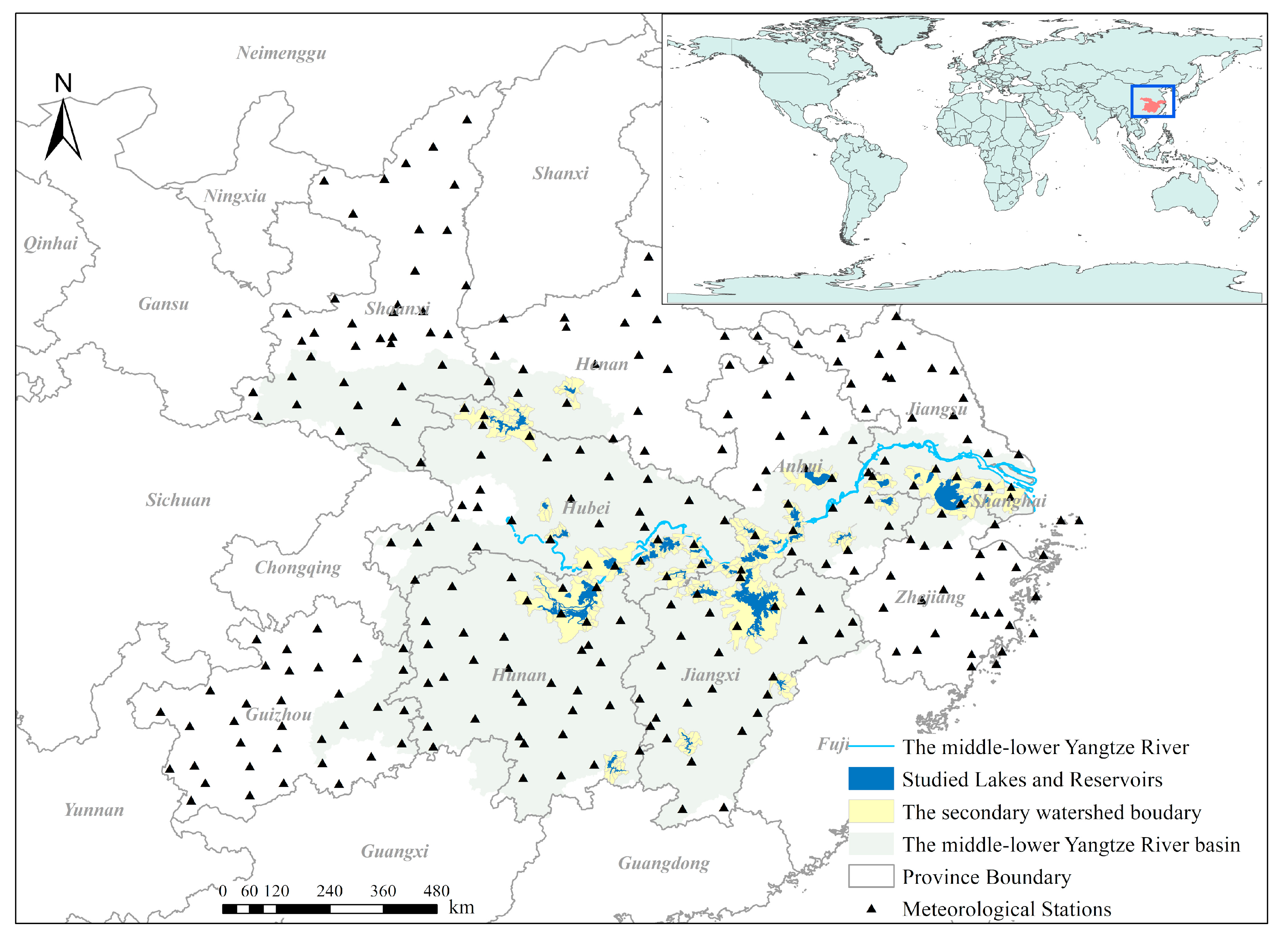
2.1. Study Area

The MLYR basin (from 29°57’N to 31°48’N, from 108°38’E to 121°52’E), a region with an area of ~785,000 km2 (Figure 1), refers to the downstream section of the Three Gorges Dam and mainly covers Hubei, Hunan, Jiangxi, Anhui, Jiangsu, and Shanghai Provinces. The region has a warm temperate and monsoon climate with four distinct seasons. The annual average temperature ranges from 14 to 18 °C, and the annual mean precipitation varies from 1000 to 1500 mm, which is mostly concentrated in the summer season.
The large lakes and reservoirs in the MLYR basin that have an area greater than 50 km2 account for just around 4% of all water bodies with an area of >1 km2, but they account for over 70% of the total water body area (see in Table 1). Thus, we focused on the yearly cyanobacterial bloom change that has occurred in lakes and reservoirs with water body areas of >50 km2. A total of 30 lakes and 10 reservoirs were included. Table 2 shows the codes, names, locations (longitude and latitude), and waterbody areas (i.e., the regions with annual inundation frequency of >25% between 2001 and 2004) of these lakes and reservoirs. The code numbers were allocated to these lakes and reservoirs in terms of their longitudes, and the numbers increase sequentially from east to west within the MLYR basin.

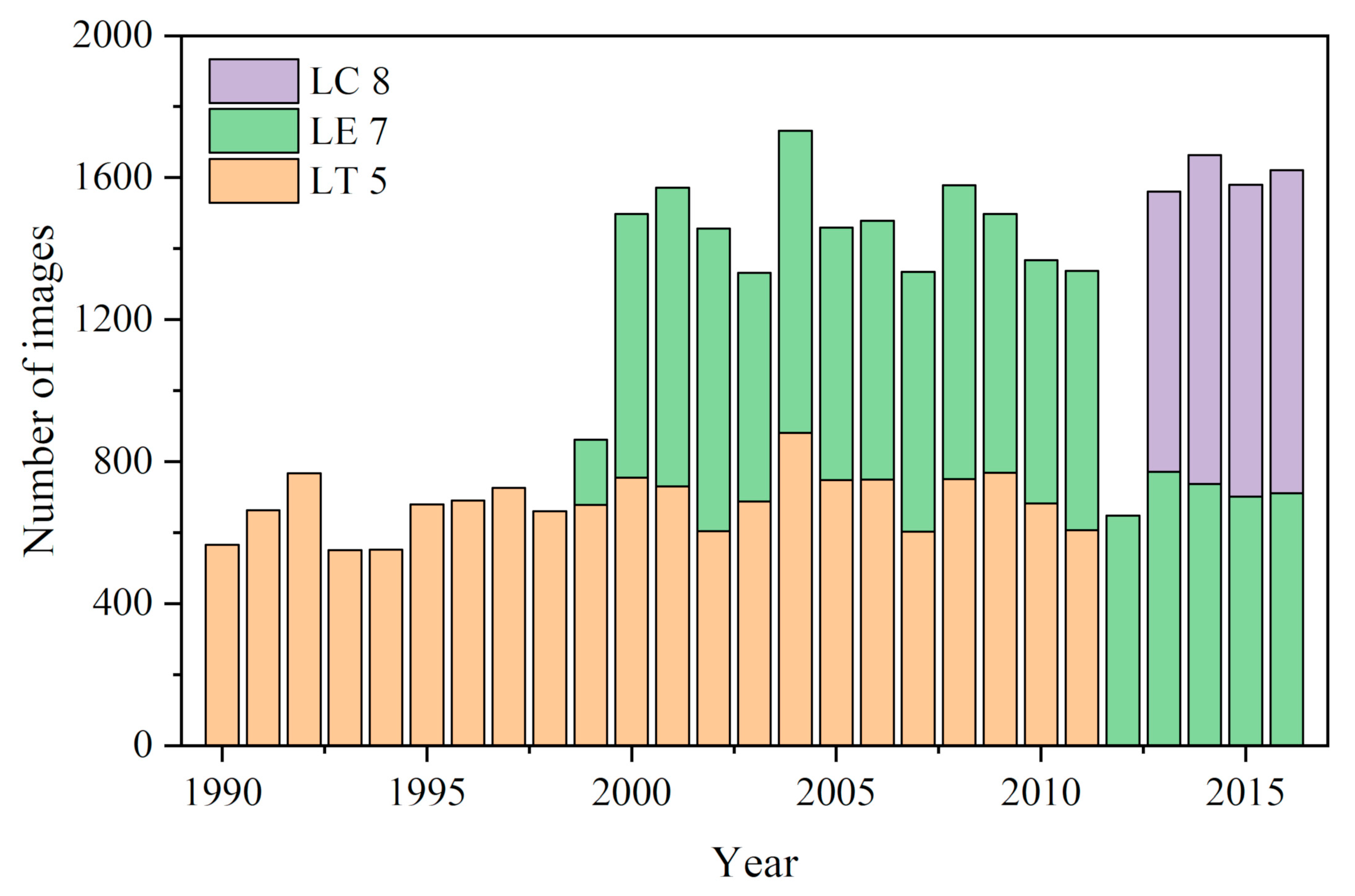
2.2. Landsat Image Data and Preprocessing

On the GEE platform, we used all the available standard Level 1 terrain corrected (L1T) products of the Landsat surface reflectance images [38] covering our study area from 1990 to 2016, including 15,097 Landsat TM images, 12,830 Landsat ETM+ images, and 3504 Landsat OLI images in total (Figure 2). The products are atmospheric corrected considering the aerosols impacts, such as molecular (Rayleigh) scattering [39]. Poor-quality observations, such as clouds, cirrus, snow, and ice observations and scan line corrector (SLC)-off gaps were excluded by a quality assessment (QA) band according to the algorithm developed by Zhu et al. [40]. Thus, all good-quality Landsat pixels were applied to form our maps.
We calculated three widely used vegetation indices (VIs), one water-related spectral index, and one algae-related spectral index from good-quality Landsat surface reflectance data. The Nominalized Difference Vegetation Index (NDVI) [41] and the Enhanced Vegetation Index (EVI) [42,43] are related to vegetation greenness; the Land Surface Water Index (LSWI) [44,45] was first used to estimate the water content of vegetation; and the Modified Normalized Difference Water Index (mNDWI) [46] is sensitive to open-surface water bodies. The Float Algal Index (FAI) [47] is an index developed especially to detect cyanobacterial blooms and was originally intended for use with MODIS, but it can also be calculated from the reflectance in the RED, NIR, and SWIR bands of Landsat images [33].
NDVI = ρ N I R ρ r e d ρ N I R + ρ r e d
EVI = 2.5 × ρ N I R ρ r e d ρ N I R + 6 × ρ r e d 7.5 × ρ b l u e + 1
LSWI = ρ N I R ρ S W I R 1 ρ N I R + ρ S W I R 1
m NDWI = ρ g r e e n ρ S W I R 1 ρ g r e e n + ρ S W I R 1
FAI = ρ N I R [ ρ r e d + ( ρ S W I R 1 ρ r e d ) × 865 655 1610 655 ]
where ρ r e d ,   ρ b l u e , ρ g r e e n ,   ρ N I R and ρ S W I R 1 are the red (630–690 nm), blue (450–520 nm), green (520–600 nm), near-infrared (NIR: 760–900 nm), and shortwave infrared (SWIR: 1550–1750 nm) bands of the Landsat TM/ETM+/OLI imagery, respectively.

2.3. Algorithms to Identify Open Surface Water Body of Lakes and Reservoirs

To map the yearly cyanobacterial bloom conditions associated with the selected lakes and reservoirs, we needed to determine the boundary of each lake and reservoir first. The mNDWI is the most widely used water index [17,46], and the optimal band analysis for Normalized Difference Water Index (NDWI) was also demonstrated with good accuracy [48]. Zou et al. [49,50] documented that the open water body can be extracted with high accuracy when the criteria ((mNDWI > NDVI or mNDWI > EVI) and (EVI < 0.1)) are satisfied. The pixels in which the annual frequency of the open water body are greater than or equal to 0.25 can be defined as surface water. We adopted this algorithm since it has been proven to be efficient in both the United States and the Poyang Lake in China [17]. Considering the impact of the Three Gorges Dam, which started operating in 2003, and the limitation of GEE (no more than 5000 images per run), we extracted the surface water region by the surface reflectance data with good-quality observations from 2001 to 2004. Then, we determined the names of the lakes and reservoirs by referring to the China Lake Scientific Database (http://lake.data.ac.cn/lake_museum/) and removed farmlands and ponds based on high-resolution images and photos incorporated into Google Earth Pro® (GE) [51]. The boundaries of the 40 selected lakes and reservoirs are shown in Figure 1.

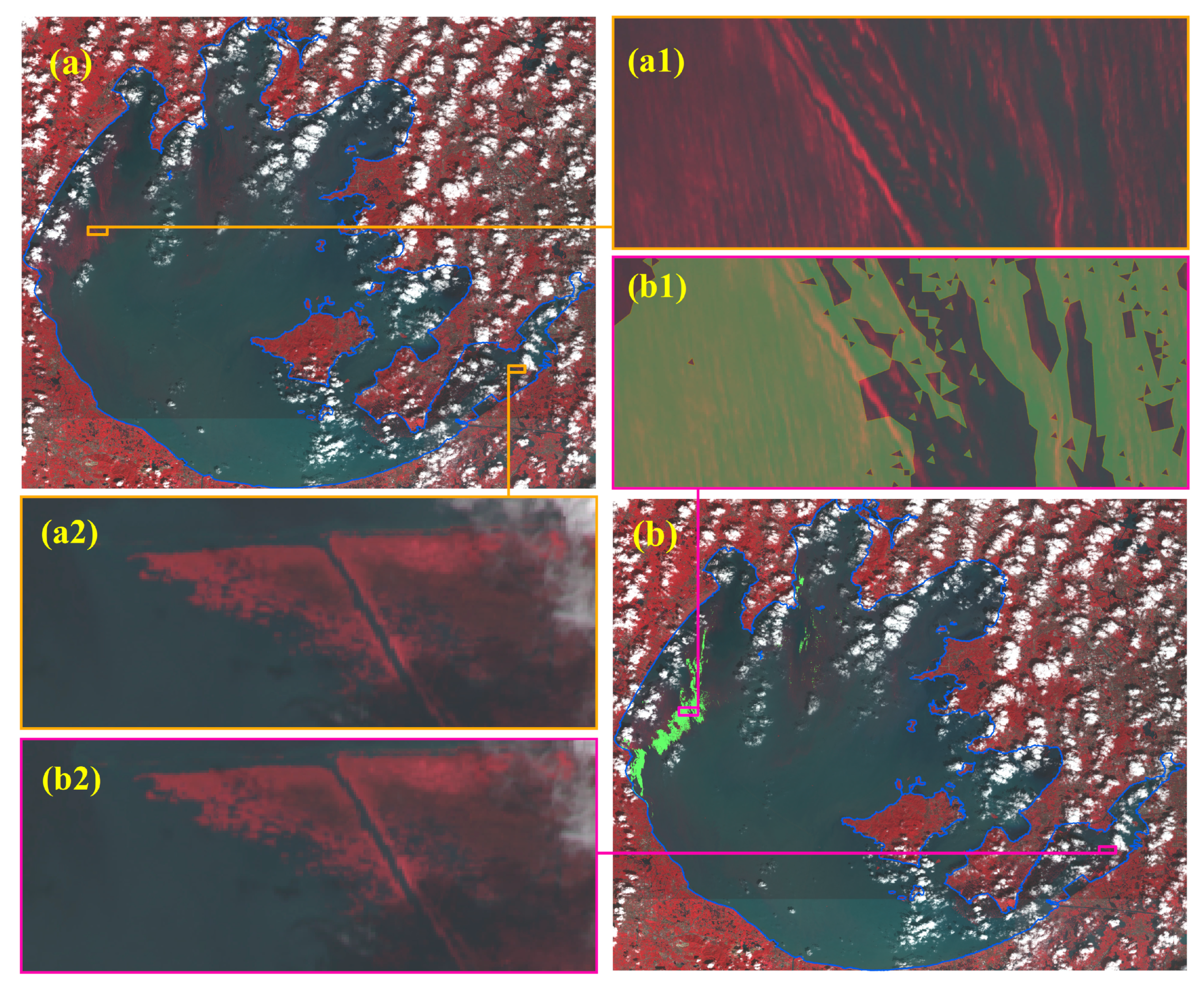
2.4. Annual Mapping of Cyanobacterial Blooms

Oyama et al. [33] found that the algorithm combining the FAI and NDWI calculated by Band 4 (RED) and Band 5 (SWIR1) (which is the LSWI) can successfully recognize cyanobacterial bloom regions when FAI > 0.05 and LSWI > 0.63 are both satisfied, which were qualitatively validated in six lakes in Japan and Indonesia. We calculated the annual occurrence times of surface cyanobacterial bloom for individual pixels in the MLYR from 1990 to 2016 and extracted the annual results in each lake and reservoir by the boundaries we produced.
We defined two parameters to assess the cyanobacterial bloom conditions and the corresponding interannual dynamics in the selected lakes and reservoirs. These parameters are the yearly cyanobacterial bloom area percentage (CAP) and the cyanobacterial bloom frequency index (CFI). The formulas are:
CAP = N C B N t o t a l × 100 %
CFI   =   i = 0 n i · N i N total
where NCB, Ntotal, i, n, and Ni are the total number of pixels with detected cyanobacterial bloom occurrence, the total number of pixels in a lake or reservoir, the occurrence times in the pixels, the maximum occurrence times in a lake or reservoir, and the total number of pixels with cyanobacterial bloom occurrence detected i times, respectively.
The CAP mainly represents the coverage of surface cyanobacterial bloom, while the CFI reflects the frequency. We performed linear regressions for the 27 years of annual data to obtain the change rate of CAP and CFI values during our study period. The change rate was considered statistically significant when the p-value associated with the linear regressions was <0.05 (t-test).

2.5. Accuracy Assessment of Annual Maps of Cyanobacterial Blooms

Ideally, in situ data are the best reference for validating the cyanobacterial blooming size, but this is difficult in practice; for example, a field survey tool (such as a boat or aircraft) disturbs the surface algae. However, comparison with concurrent higher-resolution observations is a good way to evaluate the accuracy [27]. The surface cyanobacterial blooms can be easily recognized by their spatial texture in Landsat images with a 30 m high resolution [27], so Sentinel-2 L1C images, which have an even finer resolution of 10 m, can be used for validation. Thus, the atmospherically corrected Sentinel-2 Multispectral Instrument, Level-1C data [52] at a 10 m resolution were obtained from GEE and used to validate the results. We visually examined concurrent standard false-color Sentinel-2 images to distinguish the cyanobacterial bloom region and compared it with the cyanobacterial bloom region extracted from Landsat images in the same place to validate the accuracy of the algorithm when applied to lakes located in China.

2.6. Datasets of Various Driving Factors

2.6.1. Precipitation

The monthly precipitation data from 1990 to 2016 were collected from the National Oceanic and Atmospheric Administration PERSIANN Climate Data Record (NOAA/PERSIANN-CDR) on GEE. All pixels that overlapped with individual lakes and reservoir boundaries were extracted, and the mean values were regarded as the precipitation conditions for that lake or reservoir.

2.6.2. Annual Temperature Map in the MLYR Basin

Daily air temperatures were obtained from the China Meteorological Data Sharing Service System (http://data.cma.gov). We collected data from all available meteorological stations with at least one year of complete observations during 1990–2014 in Shaanxi, Henan, Guizhou, Hunan, Hubei, Jiangsu, Jiangxi, Anhui, Zhejiang, and Shanghai. The Shuttle Radar Topography Mission (SRTM) digital elevation model (DEM) data in China, with a resolution of 1 × 1 km, was applied to perform kriging interpolation of temperature, taking the vertical temperature gradient into account.
We used the concept of active temperature (AT) in agriculture and redefined it as the sum of the daily mean temperatures above 25 °C in one year because the maximum growth rates of cyanobacteria occur at this threshold of air temperature [10]. The active temperature in our study represents the high temperatures for a specific year. Then, active temperature and yearly mean temperature (YT) were calculated for all available stations, and the results were used to produce the annual MLYR basin AT map and MLYR basin YT map by kriging interpolation. The mean values of AT (ATmean) and YT (YTmean) extracted by lake and reservoir boundaries were separately regarded as the AT and YT for the corresponding lake or reservoir in a specific year.

2.6.3. Data of Anthropogenic Activities for Each Lake and Reservoir

The population, gross domestic product in primary industries, secondary industries and tertiary industries (denoted as PGDP, SGDP, TGDP, respectively), and the amount of yearly used chemical fertilizer for farmlands (hereinafter referred to as the “fertilizer”) were obtained from the online local annual statistical books (http://tongji.cnki.net/, Anhui, Hunan, Hubei, Jiangsu, Jiangxi, Zhejiang, Henan: 1991–2017). The secondary watershed boundary extracted from a Digital Elevation Model (DEM) [53] was obtained from the Resource and Environment Data Cloud Platform.
The population, fertilizer consumption, PGDP, SGDP, and TGDP of the surrounding cities were used to quantify the impact of anthropogenic activities on cyanobacterial bloom. Besides, the regions in which secondary watershed boundaries overlapped with a lake or reservoir were regarded as the watershed of the lake or the reservoir. Considering the different impact ratios of surrounding cities due to the different distribution areas of lakes and reservoirs in cities, we calculated the overlap ratio of the watershed of the lake or reservoir with the surrounding cities. The computational method is shown in Figure 3. The ratio in individual cities was regarded as the impact ratio of anthropogenic activities from that city, and then the sum of the surrounding cities represented the population, fertilizer consumption, PGDP, SGDP, and TGDP for lakes and reservoirs.

2.7. Statistical Analysis of the Relationship between Annual Cyanobacterial Bloom Dynamics and Driving Factors

To assess the relationships between cyanobacterial bloom conditions (including CAP and CFI) and climatic changes (represented by ATmean, YTmean, and precipitation) and anthropogenic activities (represented by population, fertilizer, PGDP, SGDP, and TGDP), we constructed a series of generalized linear models (GLMs). Highly correlated variables (Spearman’s ρ > 0.8) [54] were not included in the same model. Then, we evaluated relative models supported by the information-theoretic Akaike’s information criterion corrected (AICc) for small sample sizes, and the model with the smallest AICc was selected in our analysis. A z-value was estimated for each effective variable with the GLM as well, where z-value <0.05 showed that the correlation of that variable was statistically significant.

3. Results

3.1. Accuracy Assessment for Annual Cyanobacterial Bloom Map in 2018

According to previous studies, cyanobacterial bloom has always been observed in western coastal areas, Zhushan Bay, and the Meiliang Bay, while aquatic plants have been found distributed in the East Bay in Taihu Lake [30]. The results of cyanobacterial bloom coverage extracted according to FAI > 0.05 and LSWI > 0.63 from Landsat were consistent with the visually determined results from Sentinel-2 imagery (Figure 4a1,b1), confirming that we did not falsely identify aquatic plants as cyanobacterial bloom (Figure 4a2,b2). This indicates that the FAI- and LSWI-based algorithm can also be applied to the detection of cyanobacterial bloom regions in water bodies located in China.

3.2. Spatiotemporal Changes in Cyanobacterial Blooms in 1990–2016

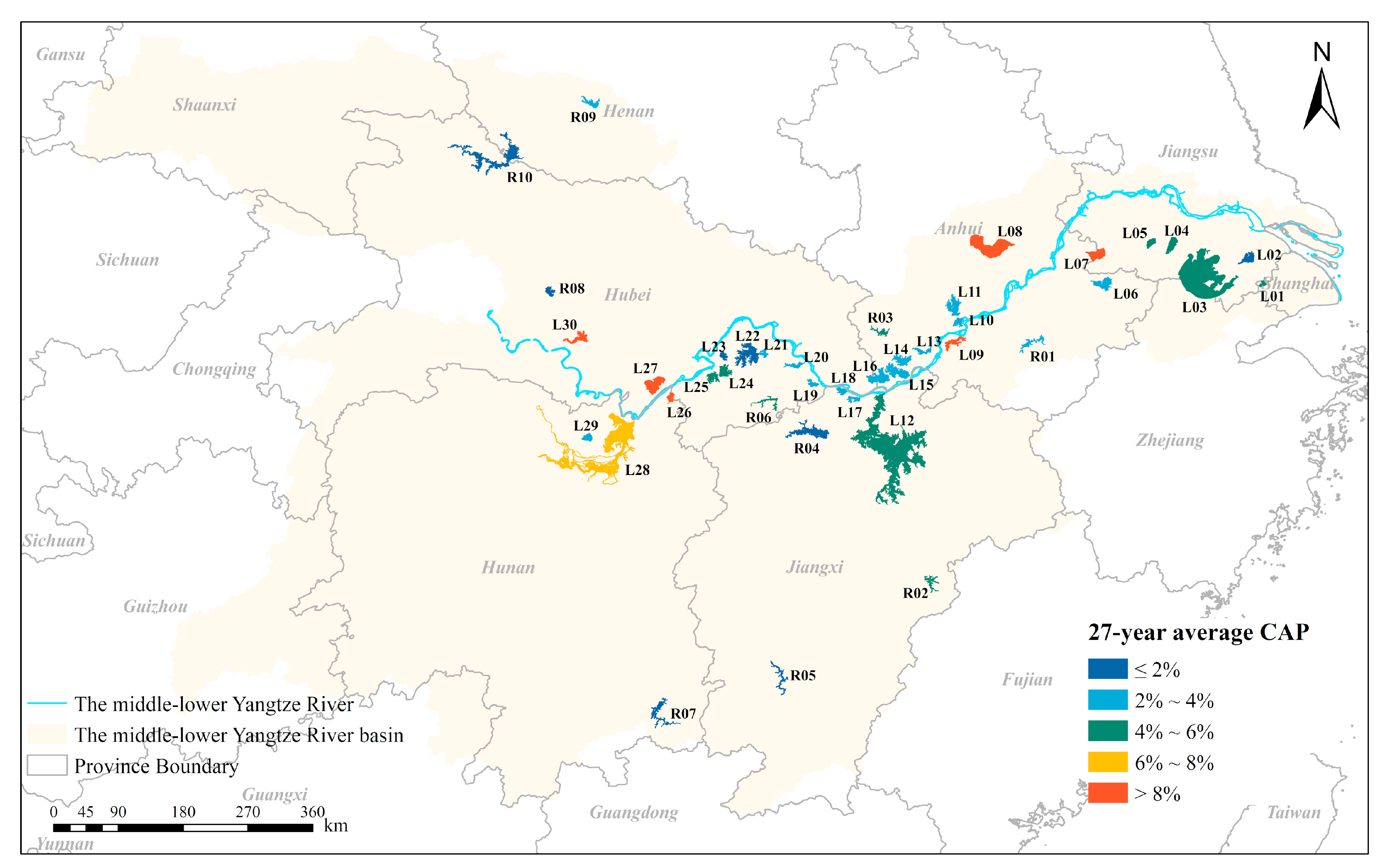
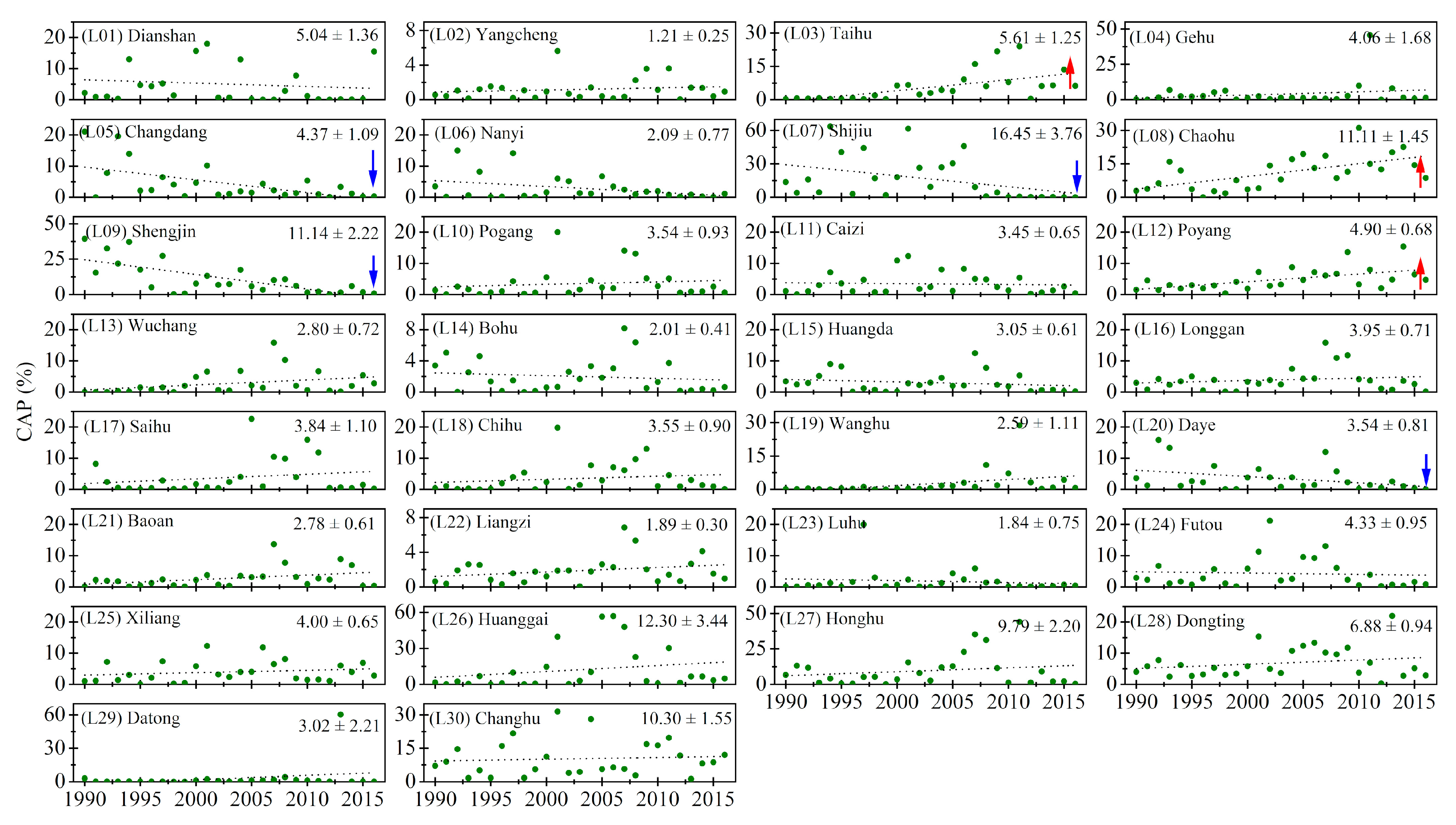
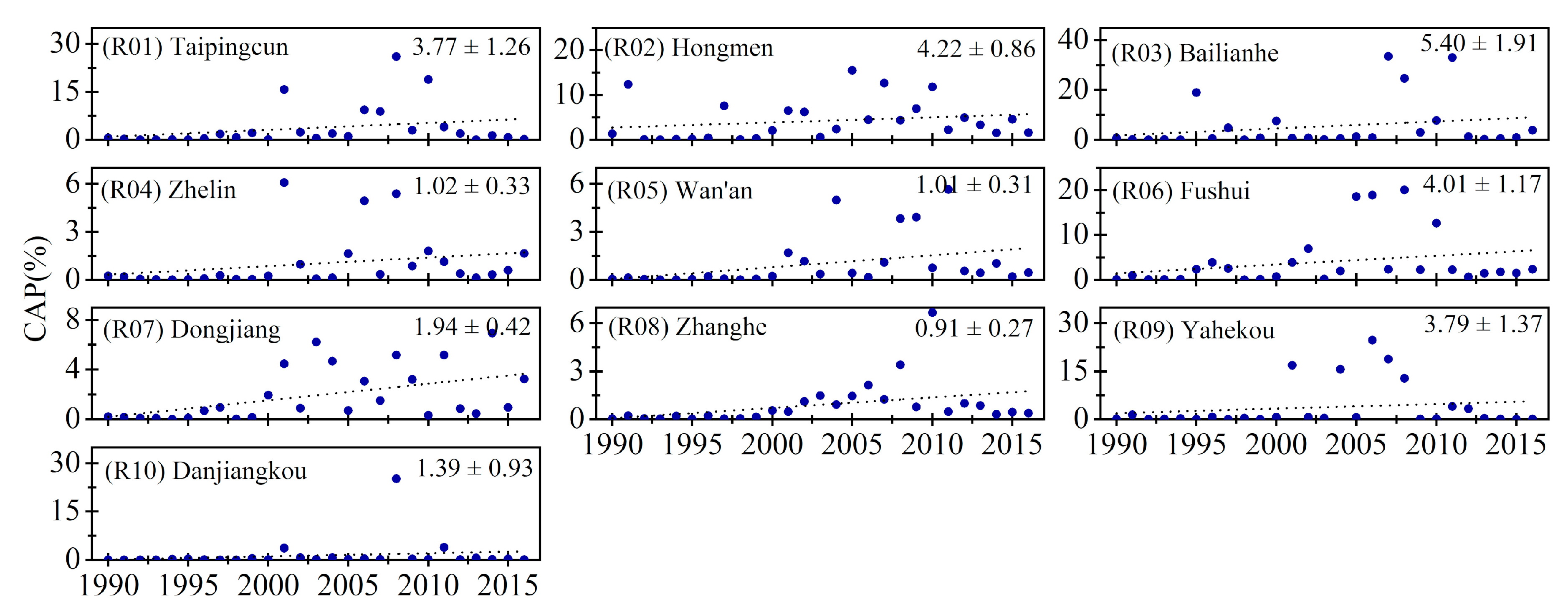
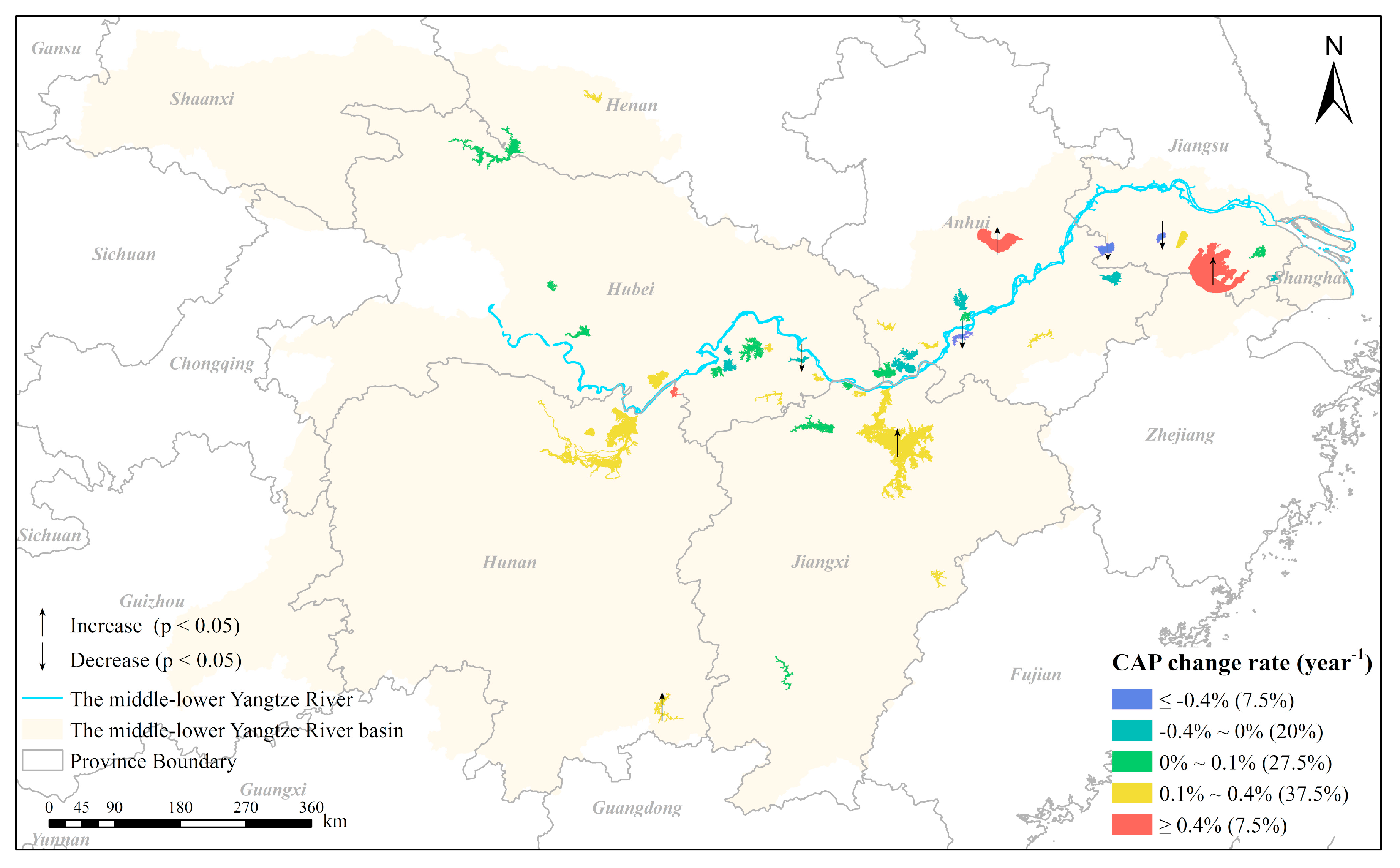
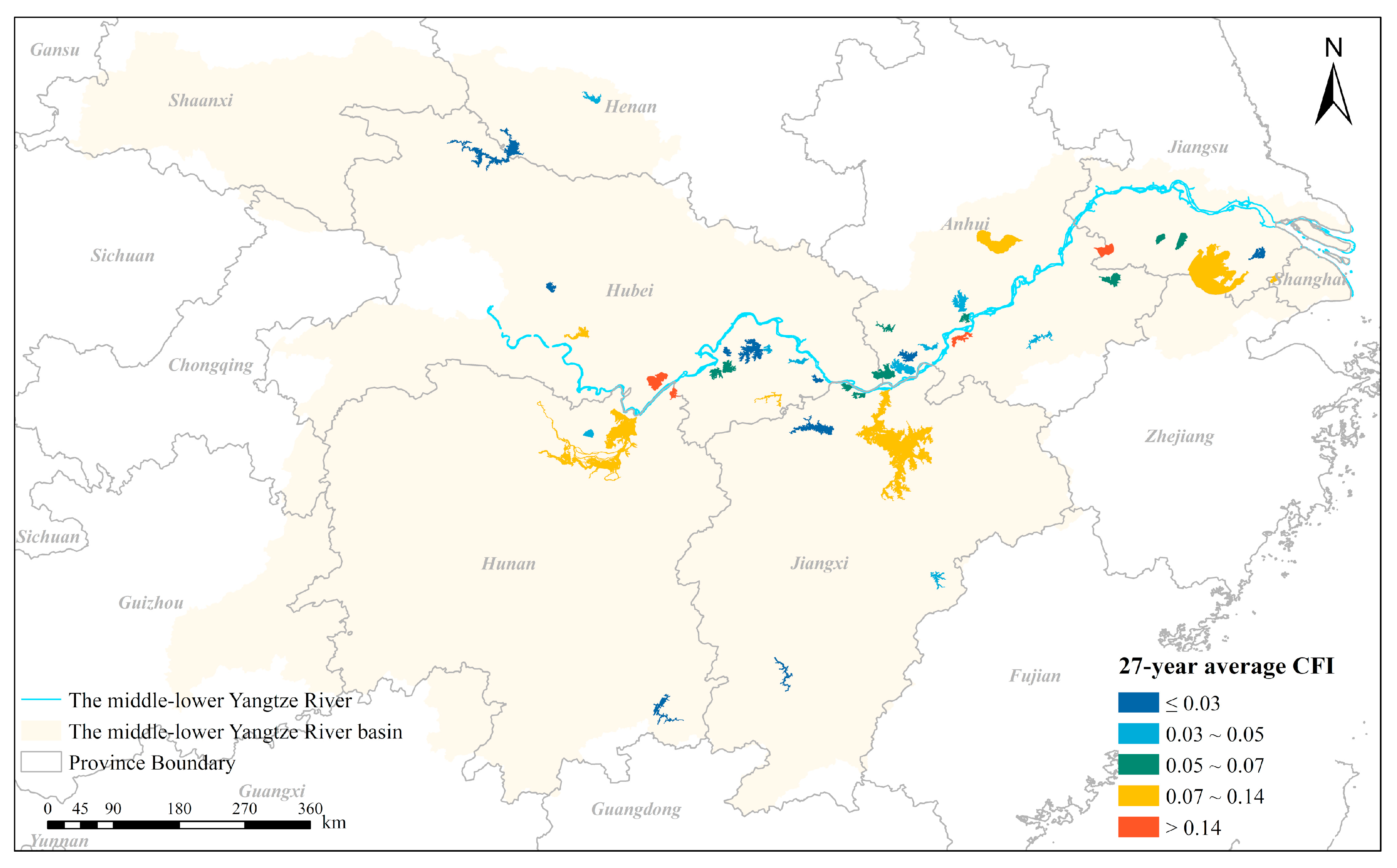
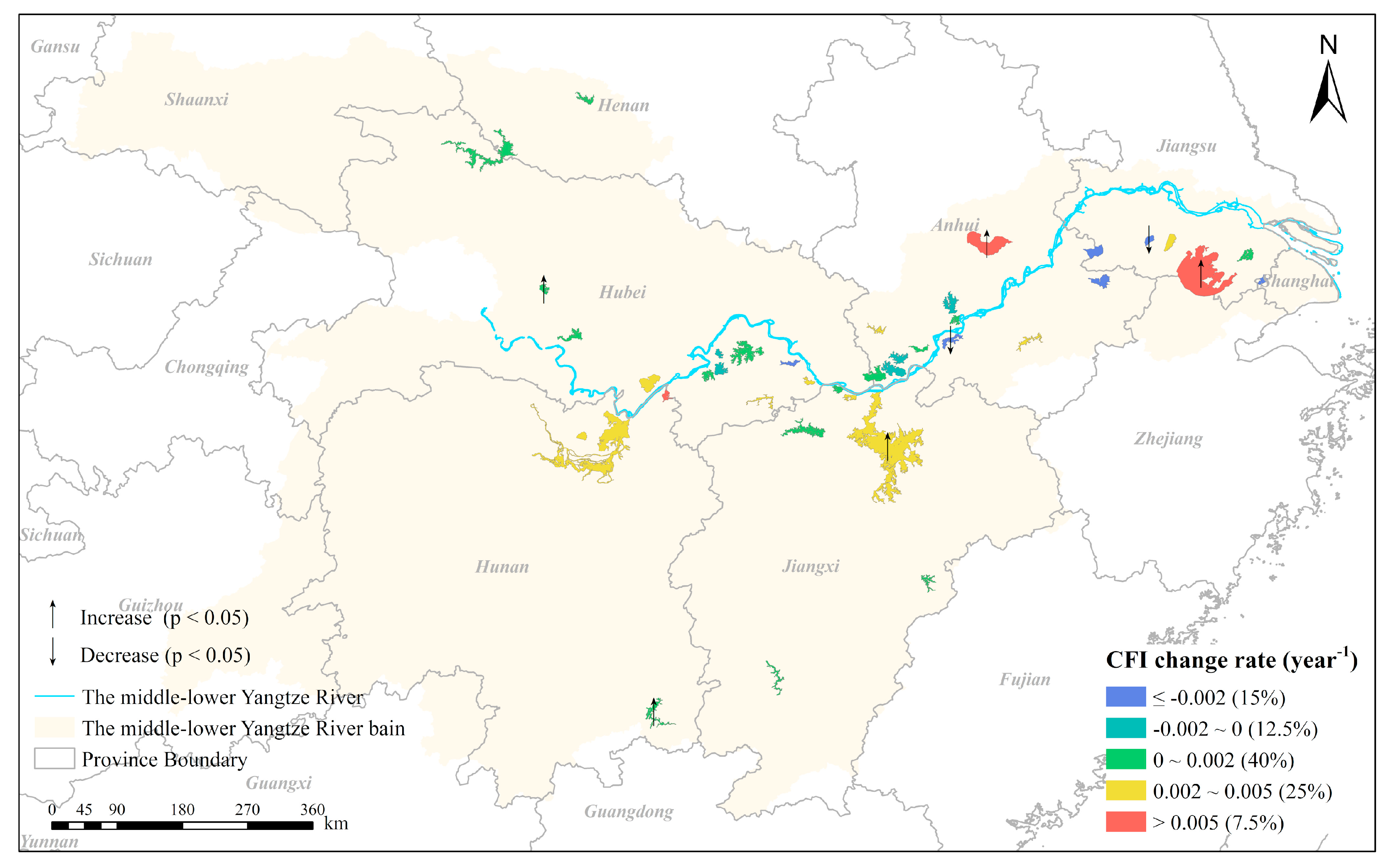
3.2.1. Temporal and Spatial Distributions of Cyanobacterial Bloom

The CAP climatology data of all 40 selected lakes and reservoirs over 27 years are displayed in Figure 5, and the spatial patterns of the CAP distributions can be observed. On average, the yearly cyanobacterial bloom area percentage of lakes ranged from 1.21% (Yangcheng Lake) to 16.44% (Shijiu Lake), and that of reservoirs varied from 0.91% (Zhanghe Reservoir) to 5.40% (Bailianhe Reservoir) from 1990 to 2016 (Figure 5, Figure 6 and Figure 7). Overall, of the 30 lakes, only 10% had 27-year mean CAP values of ≤2%; 43.3% were between 2% and 4%; 23.3% ranged from 4% to 6%; 3.3% were between 6% and 8%; and 20% were >8%. Of the 10 reservoirs, 50%, 20%, and 30% had values of ≤2%, 2–4%, and 4–6%, respectively.
The changing trends of interannual CAP for each lake and reservoir from 1990 to 2016 (Figure 6 and Figure 7) and the change rates for all the lakes and reservoirs with spatial distributions are displayed by color shading in Figure 8. When the CAP change rates were classified into five levels (≤−0.4% year−1, −0.4% to 0% year−1, 0–0.1% year−1, 0.1–0.4% year−1, and >0.4% year−1), the corresponding proportions of each level were 7.5%, 20%, 27.5%, 37.5%, and 7.5% of the studied lakes and reservoirs, respectively. The CAPs for about 63% of the lakes (19/30) and all reservoirs showed increasing trends, and the most pronounced increase was observed in Chaohu Lake (L05, with a change rate of 0.57% year−1), while the greatest decrease was found in Shengjin Lake (L09, with a change rate of −1.04% year−1). Three lakes and one reservoir showed statistically significant increasing trends, while four lakes had CAPs that decreased significantly during the study period.

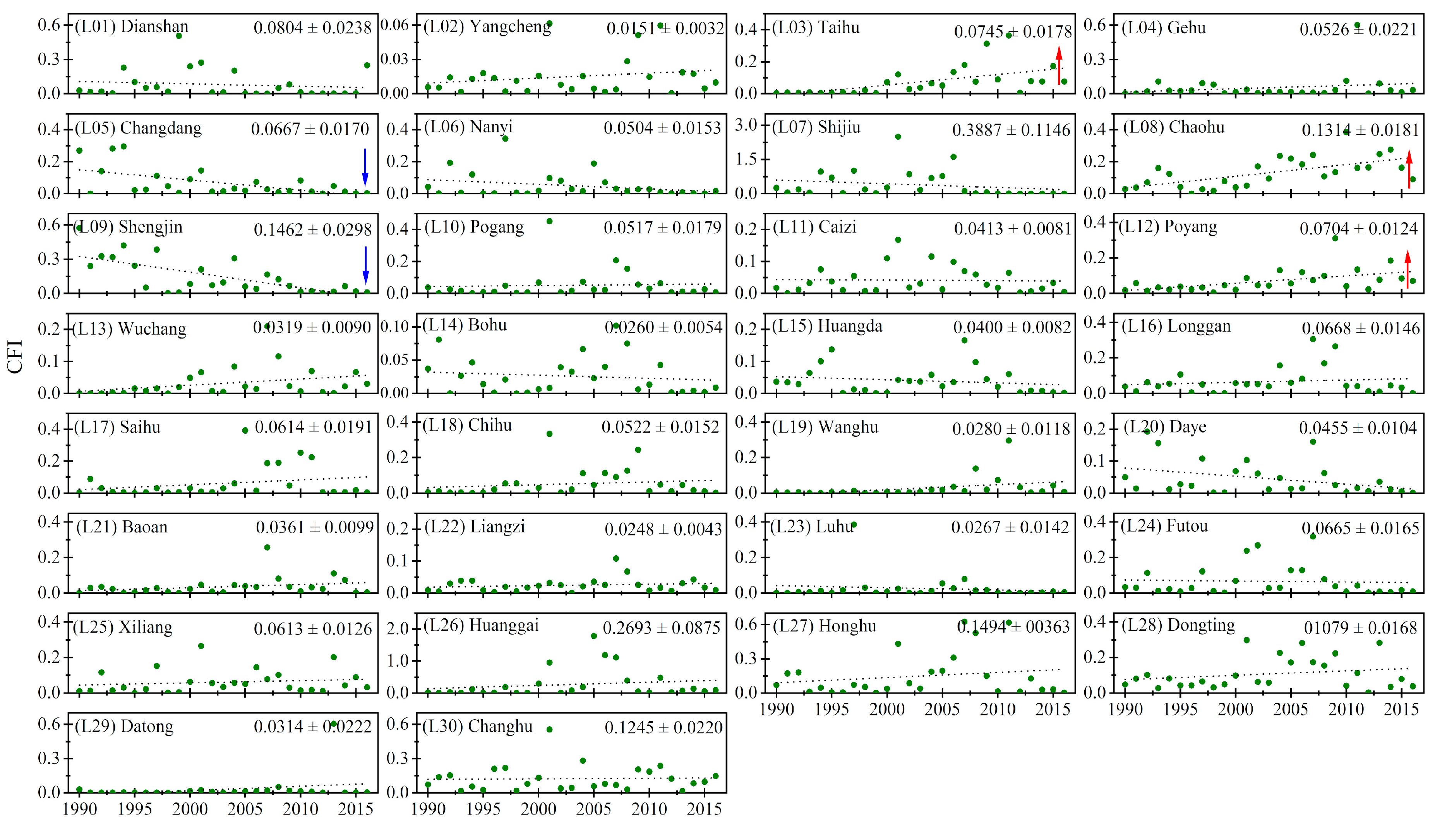
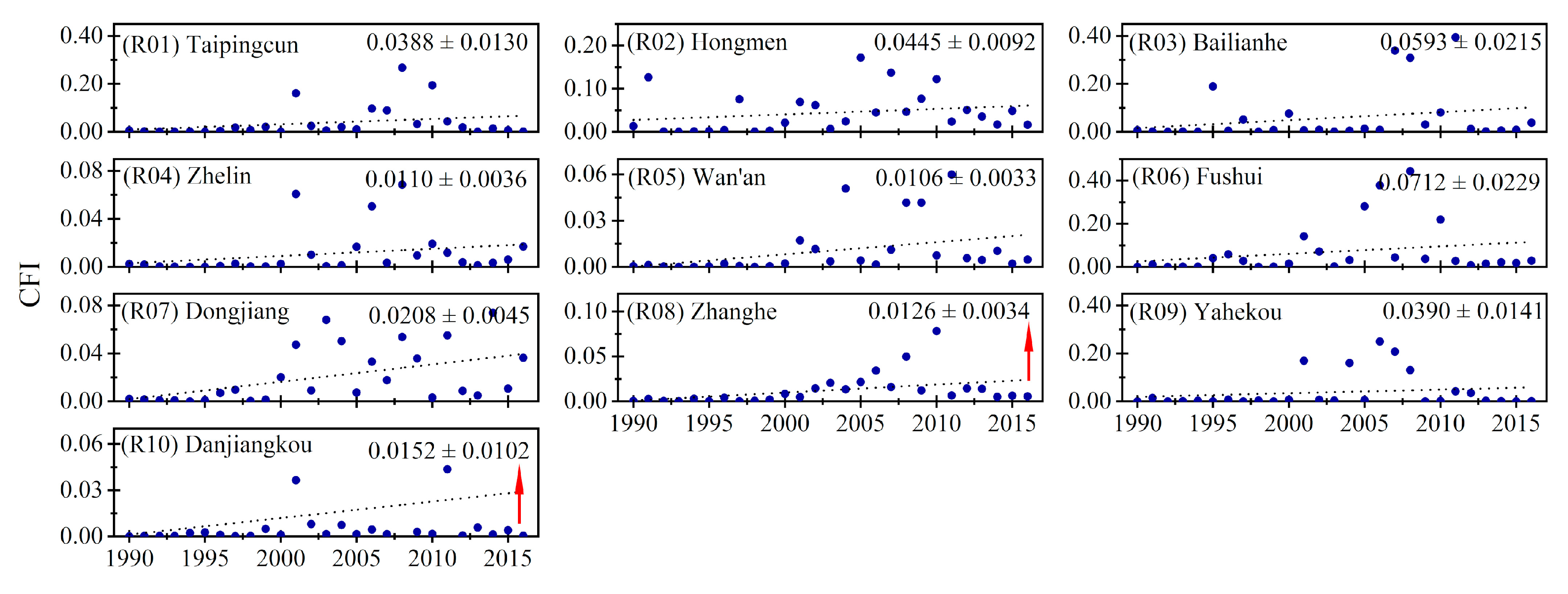
3.2.2. Interannual Changes in the Frequency of Cyanobacterial Bloom

The 27-year mean CFIs of each lake and reservoir are presented in Figure 9. Specifically, the climatological CFI of lakes varied from 0.015 (Yangcheng Lake) to 0.389 (Shijiu Lake), and that of reservoirs ranged from 0.011 (Wan’an Reservoir) to 0.071 (Fushui Reservoir) during the study period (Figure 9, Figure 10 and Figure 11). In general, of the 30 lakes, only 16.7% had a 27-year mean CFI value of ≤0.03; 20% were between 0.03 and 0.05; 30% ranged from 0.05 to 0.07; 20% were between 0.07 and 0.14; and 13.3% were >0.14. Of the 10 reservoirs, 50%, 30%, 10% and 10% had values in the previously mentioned five levels, respectively.
The interannual variation trends of the CFI and the associated change rates of CFI from 1990 to 2016 for all lakes and reservoirs were analyzed and are displayed in Figure 10 and Figure 11, respectively. With the changing rates of CFI (Figure 12) categorized as five levels (≤−0.002 year−1, −0.002 to 0 year−1, 0–0.0.002 year−1, 0.002–0.005 year−1, and >0.005 year−1), the number of selected lakes and reservoirs that fell into each level accounted for 15%, 12.5%, 40%, 25% and 7.5%. Similar to the results for CAP, 60% of lakes (18/30) and all reservoirs showed increasing trends in their CFIs, and the greatest increasing trend was found in Huanggai Lake (L26, with a change rate of 0.010 year−1), whereas the most pronounced decrease was observed in Shijiu Lake (L09, with a change rate of −0.016 year−1). Three of the lakes and two of the reservoirs showed statistically significant increasing trends in the CFI in 1990–2016. On the contrary, statistically significant decreasing trends in the CFI were observed in only two lakes, and these lakes were found in the middle and eastern MLYR basin.

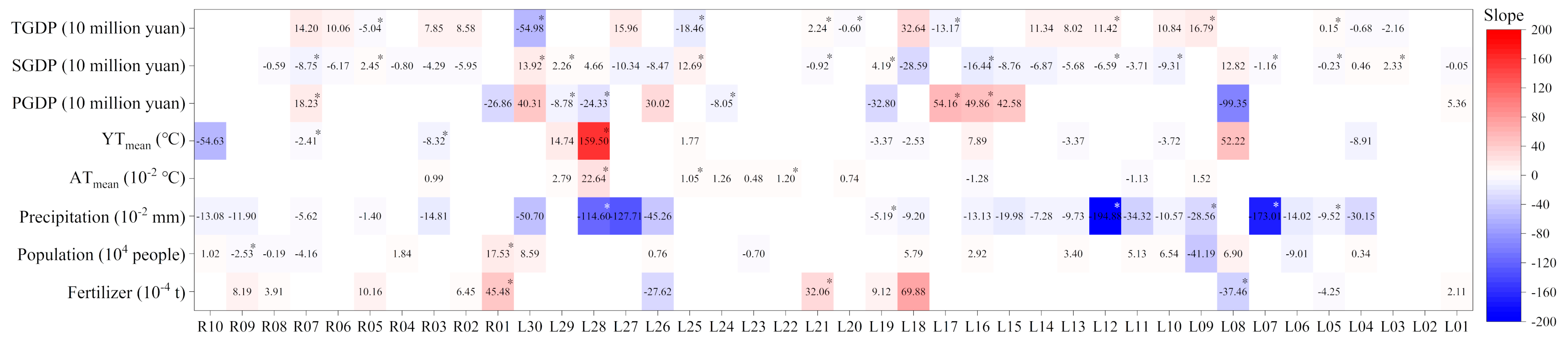
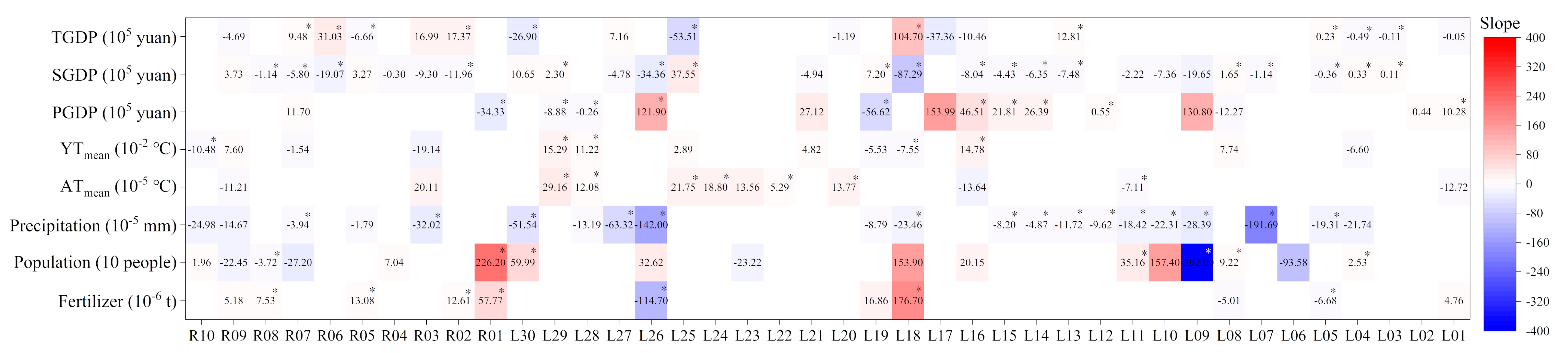
3.3. Major Driving Factors for the Observed Spatiotemporal Dynamics of Cyanobacterial Blooms from 1990 to 2016

To further investigate the relationship between cyanobacterial bloom and climatic and anthropogenic factors, a relative model of the lakes and reservoirs with the eight above-mentioned driving factors was analyzed. The regression coefficients (denoted as “Slope”) between explanatory variables and the CAP and CFI are displayed in Figure 13 and Figure 14, respectively.
The response of the annual coverage area (represented by CAP) and frequency (represented by CFI) of cyanobacterial bloom to the eight driving factors varied differently for lakes and reservoirs. Forty percent of the reservoirs (4/10) exhibited correlations between coverage area and fertilizer consumption while just 7% of the lakes (2/30) had this correlation. The results for the frequency were almost the same. Besides, the correlations for all reservoirs and lakes were positive, and two of the reservoirs showed significantly positive correlations (z < 0.05). The results indicated that reservoirs were more inclined to be affected by the use of fertilizer by surrounding farmlands in one year than lakes in the MLYR basin. As a whole, the population distribution surrounding the lakes and reservoirs seemed to show a weak relationship with cyanobacterial blooms, where about 20% of the lakes and 10% of reservoirs were correlated. Compared with reservoirs, the GDP (including PGDP, SGDP, and TGDP) seemed to be more correlated with the cyanobacterial bloom coverage area and frequency in lakes. Our results demonstrated that the development of tertiary industries might be related to the cyanobacterial bloom increase while the development of secondary industries may be related to its decrease. Overall, GDP had little effect on cyanobacterial blooms.
In contrast, the precipitation and air temperature (quantified by ATmean and YTmean) were more relevant to cyanobacterial blooms. Approximately 50% of the lakes and reservoirs displayed a negative correlation with the annual coverage area and frequency of cyanobacterial blooms, where eleven lakes showed a statistically significant negative relationship, which demonstrated that an increase in precipitation in a lake and reservoir region might be related to the reduction in cyanobacterial blooms. Conversely, the increase in yearly mean temperature and extremely high temperature in a specific year might be linked with the increase in cyanobacterial blooms. We found that near 30% of lakes and 10% of reservoirs exhibited a positive correlation between the ATmean and the cyanobacterial bloom coverage area and frequency, where approximately half of the lakes showed a significant relationship. The YTmean showed a lower correlation with cyanobacterial blooms, but virtually all were positive and statistically significant. As a whole, the cyanobacterial bloom seemed to be more related to meteorological factors.

4. Discussion

4.1. Detection and Mapping of Cyanobacterial Blooms

In this study, we illustrate that the algorithm produced by Oyama et al. [33] that distinguishes a cyanobacterial bloom region from Landsat data can also be well applied to water bodies in China. Many researchers have conducted the cyanobacterial bloom monitoring in several large and vital lakes located in the MLYR basin, such as Taihu Lake and Chaohu Lake. Duan et al. [20,55] demonstrated that the occurrences of algal blooms in Taihu Lake became increasingly severe from 1987 to 2011, mainly reflected by an increased frequency, duration, and coverage. The same tendency was also found in Chaohu Lake from 2000 to 2013 [25]. Our results for Taihu and Chaohu Lakes are consistent with the previous results. We also verified the results of deteriorating water quality and eutrophication in Poyang and Dongting Lakes [18,23]. Moreover, we completed the monitoring of dynamics of cyanobacterial blooms in many other large lakes and reservoirs located in the MLYR basin from 1990 to 2016, as this was lacking in previous studies.
Ideally, all time-series images would detect every cyanobacterial bloom event in a specific year during our observation period. Nevertheless, with a 16 day revisit period, Landsat satellites can only partially obtain the information of full cyanobacterial bloom conditions in a year, and some blooming events may be missed. Thus, the yearly maximum area coverage and frequency of cyanobacterial bloom in this study have some limitations on the accuracy. However, it is still certain that the proposed approach analyzed by Landsat can be effectively used for long-term cyanobacterial bloom monitoring because the changing trend and main driving forces of cyanobacterial bloom in lakes and reservoirs are consistent with previous studies.

4.2. Driving Factors of Cyanobacterial Bloom Dynamics

The increase in both phytoplankton biomass and the frequency of cyanobacterial blooms have been associated with the overall increase in nutrient inputs from agricultural, urban, and industrial sources [10]. The availability and composition of nitrogen (N) and phosphorus (P) in freshwater bodies control the production and compositions of phytoplankton communities [9,11,56]. Fertilizer consumption and wastewater discharge were identified as main ways through which anthropogenic activities import nutrients into surrounding water bodies [5,10,57]. Compared with the reservoirs, the lakes showed less correlation with fertilizer consumption (Figure 13 and Figure 14). This might be attributable to the different trophic states, as Wang et al. [18] demonstrated that, in the middle–lower Yangtze region, large lakes were mainly eutrophic, while the reservoirs studied were mesotrophic. Since the population and GDP affect the process of cyanobacterial generation or bloom indirectly, they showed no significant regularity in their effects. However, the significant decrease in blooms in several lakes was related to the population or GDP, and this might be attributable to the effects of the aggressive recovery strategy for environmental protection proposed by the government, especially after the severe cyanobacterial bloom in Taihu Lake in 2007 [6]. For instance, researchers have revealed that the River Chief Policy could improve the water quality of water bodies in the Yangtze River Economic Belt, and the positive effect may be relevant to industrial structural upgrades and industrial waste discharge control especially in cities with higher GDP [58]. Nevertheless, a more detailed investigation should be conducted in the future in the lakes with a significant decrease in blooms, such as Shengjin Lake, Shijiu Lake, Daye Lake, and Changdang Lake.
In addition to the promotion of blooms due to nutrient over-enrichment, climate change, including rising global temperatures and changing precipitation patterns, also affected the process of cyanobacterial blooms [10,11,59]. High temperatures increase the generation of phytoplankton and alter their vertical stratification, which contributes to the surface accumulation of algae [56,59]. Our results show that high temperatures in a year were correlated with the increase in cyanobacterial bloom, which is in agreement with previous studies. Besides, we found that precipitation was related to the decrease in cyanobacterial bloom. In past efforts, precipitation events were hypothesized to enrich the nutrients of water bodies through surface runoff or promote flushing by freshwater discharge, which would increase or (in the short-term) prevent blooms, respectively [8,9]. Our results confirm the latter. Precipitation is usually concentrated in spring and summer in the MLYR basin when the temperature is extremely suitable for the generation of cyanobacteria. Thus, precipitation events can interrupt long periods of diurnal stratifications, increase the disruption of water bodies, dilute the concentration of nutrients in water [56], and therefore, decrease the occurrence of bloom. Overall, the cyanobacterial bloom is complex, it is related to a mixture of anthropogenic and climatic factors and displays different combination patterns in different lakes and reservoirs.

4.3. Implications

At present, this work is restrained by the quantity and quality of Landsat images. Nonetheless, along with the development of remote sensing technology, Sentinel-2 [60,61,62,63] and Worldview 3 [64]—two of many multi-spectral sensors with higher temporal and spatial resolutions—are potential sources of available data for land use/cover change monitoring with higher precision. In the future, we could combine more image data (e.g., Landsat, Sentinel-1 and 2, Worldview 3) to build a more accurate and scientifically recognized database of cyanobacterial bloom events in China and worldwide. The algorithm produced by Oyama et al. [33] can be applied effectively to the many lakes distributed in Japan, Indonesia, and China; thus, we could attempt to discover the dynamics of cyanobacterial blooms in water bodies around the world in the future. Besides, the process of cyanobacterial bloom is so complex that we still need more field records to enrich our understanding of it. If successful, we might find an appropriate approach to defeat the green monster.

5. Conclusions

In this study, Landsat images were processed using FAI and LSWI by the GEE platform to explore the spatial distributions and temporal dynamics of cyanobacterial blooms over the last 27 years in large lakes and reservoirs distributed in the MLYR basin. The results illustrate the reliability of long-term cyanobacterial bloom monitoring by Landsat satellites, and the approach can be utilized by changing trend analysis. The interannual variation and trends of the cyanobacterial bloom coverage area and frequency from 1990 to 2016 were analyzed. All reservoirs and more than 60% of lakes tended to increase in the coverage area and frequency of cyanobacterial blooms under the pressures of climate change and anthropogenic interferences. Compared with lakes, reservoirs were more inclined to be affected by fertilizer consumption from their regional surroundings. High temperatures appear to increase cyanobacterial blooms while precipitation in the lake and reservoir region might somewhat alleviate blooms. With results that can be traced back to the 20th century, this study provides baseline information on cyanobacterial bloom changes in 30 large lakes and 10 large reservoirs in the middle–lower Yangtze River basin. Thus, the findings could serve as a reference for future environmental monitoring and governance of these lakes and reservoirs.

Author Contributions

Conceptualization, J.Z. and B.Z.; methodology, J.Z., X.W., Q.Z., X.X. and B.Z.; software, Q.Z.; validation, J.Z. and X.W.; formal analysis, J.Z., X.W. and X.X.; investigation, J.Z.; resources, J.M. and B.Z.; data curation, J.Z., X.W., Q.Z., X.X. and J.M.; writing–original draft, J.Z.; writing–review & editing, J.Z., X.W., Q.Z., X.X., J.M. and B.Z.; visualization, J.Z.; supervision, Q.Z., X.X. and J.M.; project administration, B.Z.; funding acquisition, B.Z.

Funding

This work was funded by the National Key Research and Development Program of China (grant number 2018YFD0900806), and the Field Station Union Project of Chinese Academy of Sciences (KFJ-SW-YW026).

Acknowledgments

We appreciate the assistance of Zheng Zhou for accessing the Google Earth Engine. We also gratefully thank all the reviewers for their valuable comments on the earlier versions of the manuscript.

Conflicts of Interest

The authors declare no conflict of interest.

References

  1. Herdendorf, C.E. Large Lakes of the World. J. Great Lakes Res. 1982, 8, 379–412. [Google Scholar] [CrossRef]
  2. Hou, X.; Feng, L.; Duan, H.; Chen, X.; Sun, D.; Shi, K. Fifteen-year monitoring of the turbidity dynamics in large lakes and reservoirs in the middle and lower basin of the Yangtze River, China. Remote Sens. Environ. 2017, 190, 107–121. [Google Scholar] [CrossRef]
  3. Li, X.; Yu, X.; Jiang, L.; Li, W.; Liu, Y.; Hou, X. How important are the wetlands in the middle–lower Yangtze River region: An ecosystem service valuation approach. Ecosyst. Serv. 2014, 10, 54–60. [Google Scholar] [CrossRef]
  4. Torbick, N.; Hession, S.; Hagen, S.; Wiangwang, N.; Becker, B.; Qi, J. Mapping inland lake water quality across the Lower Peninsula of Michigan using Landsat TM imagery. Int. J. Remote Sens. 2013, 34, 7607–7624. [Google Scholar] [CrossRef]
  5. Fang, C.; Song, K.; Li, L.; Wen, Z.; Liu, G.; Du, J.; Shang, Y.; Zhao, Y. Spatial variability and temporal dynamics of HABs in Northeast China. Ecol. Indic. 2018, 90, 280–294. [Google Scholar] [CrossRef]
  6. Guo, L. ECOLOGY: Doing Battle With the Green Monster of Taihu Lake. Science 2007, 317, 1166. [Google Scholar] [CrossRef] [PubMed]
  7. Ho, J.C.; Stumpf, R.P.; Bridgeman, T.B.; Michalak, A.M. Using Landsat to extend the historical record of lacustrine phytoplankton blooms: A Lake Erie case study. Remote Sens. Environ. 2017, 191, 273–285. [Google Scholar] [CrossRef]
  8. Michalak, A.M.; Anderson, E.J.; Beletsky, D.; Boland, S.; Bosch, N.S.; Bridgeman, T.B.; Chaffin, J.D.; Cho, K.; Confesor, R.; Daloglu, I.; et al. Record-setting algal bloom in Lake Erie caused by agricultural and meteorological trends consistent with expected future conditions. Proc. Natl. Acad. Sci. USA 2013, 110, 6448–6452. [Google Scholar] [CrossRef] [PubMed] [Green Version]
  9. Paerl, H.W.; Hall, N.S.; Calandrino, E.S. Controlling harmful cyanobacterial blooms in a world experiencing anthropogenic and climatic-induced change. Sci. Total Environ. 2011, 409, 1739–1745. [Google Scholar] [CrossRef] [PubMed]
  10. Paerl, H.W.; Otten, T.G. Harmful Cyanobacterial Blooms: Causes, Consequences, and Controls. Microb. Ecol. 2013, 65, 995–1010. [Google Scholar] [CrossRef] [PubMed]
  11. Wells, M.L.; Trainer, V.L.; Smayda, T.J.; Karlson, B.S.O.; Trick, C.G.; Kudela, R.M.; Ishikawa, A.; Bernard, S.; Wulff, A.; Anderson, D.M.; et al. Harmful algal blooms and climate change: Learning from the past and present to forecast the future. Harmful Algae 2015, 49, 68–93. [Google Scholar] [CrossRef] [PubMed] [Green Version]
  12. Cai, X.; Feng, L.; Hou, X.; Chen, X. Remote Sensing of the Water Storage Dynamics of Large Lakes and Reservoirs in the Yangtze River Basin from 2000 to 2014. Sci. Rep. 2016, 6, 36405. [Google Scholar] [CrossRef] [PubMed] [Green Version]
  13. Wang, J.; Sheng, Y.; Tong, T.S.D. Monitoring decadal lake dynamics across the Yangtze Basin downstream of Three Gorges Dam. Remote Sens. Environ. 2014, 152, 251–269. [Google Scholar] [CrossRef]
  14. Yang, X.; Lu, X.X. Delineation of lakes and reservoirs in large river basins: An example of the Yangtze River Basin, China. Geomorphology 2013, 190, 92–102. [Google Scholar] [CrossRef]
  15. Qin, Y.; Xiao, X.; Dong, J.; Chen, B.; Liu, F.; Zhang, G.; Zhang, Y.; Wang, J.; Wu, X. Quantifying annual changes in built-up area in complex urban-rural landscapes from analyses of PALSAR and Landsat images. ISPRS J. Photogramm. Remote Sens. 2017, 124, 89–105. [Google Scholar] [CrossRef] [Green Version]
  16. Wang, Q.; Xiao, Q.; Liu, C.; Wang, K.; Ye, M.; Lei, A.; Song, X.; Kohata, K. Effect of reforestation on nitrogen and phosphorus dynamics in the catchment ecosystems of subtropical China: The example of the Hanjiang River basin. J. Sci. Food Agric. 2012, 92, 1119–1129. [Google Scholar] [CrossRef]
  17. Wang, Y.; Ma, J.; Xiao, X.; Wang, X.; Dai, S.; Zhao, B. Long-Term Dynamic of Poyang Lake Surface Water: A Mapping Work Based on the Google Earth Engine Cloud Platform. Remote Sens. 2019, 11, 313. [Google Scholar] [CrossRef]
  18. Wang, S.; Li, J.; Zhang, B.; Spyrakos, E.; Tyler, A.N.; Shen, Q.; Zhang, F.; Kuster, T.; Lehmann, M.K.; Wu, Y.; et al. Trophic state assessment of global inland waters using a MODIS-derived Forel-Ule index. Remote Sens. Environ. 2018, 217, 444–460. [Google Scholar] [CrossRef] [Green Version]
  19. Duan, H.; Tao, M.; Loiselle, S.A.; Zhao, W.; Cao, Z.; Ma, R.; Tang, X. MODIS observations of cyanobacterial risks in a eutrophic lake: Implications for long-term safety evaluation in drinking-water source. Water Res. 2017, 122, 455–470. [Google Scholar] [CrossRef]
  20. Duan, H.; Loiselle, S.A.; Zhu, L.; Feng, L.; Zhang, Y.; Ma, R. Distribution and incidence of algal blooms in Lake Taihu. Aquat. Sci. 2015, 77, 9–16. [Google Scholar] [CrossRef]
  21. Liu, J.; Fang, S. Comprehensive evaluation of the potential risk from cyanobacteria blooms in Poyang Lake based on nutrient zoning. Environ. Earth Sci. 2017, 76, 342. [Google Scholar] [CrossRef]
  22. Liu, X.; Qian, K.; Chen, Y.; Gao, J. A comparison of factors influencing the summer phytoplankton biomass in China’s three largest freshwater lakes: Poyang, Dongting, and Taihu. Hydrobiologia 2017, 792, 283–302. [Google Scholar] [CrossRef]
  23. Liu, X.; Li, Y.-L.; Liu, B.-G.; Qian, K.-M.; Chen, Y.-W.; Gao, J.-F. Cyanobacteria in the complex river-connected Poyang Lake: Horizontal distribution and transport. Hydrobiologia 2016, 768, 95–110. [Google Scholar] [CrossRef]
  24. Wang, M.; Shi, W. Satellite-Observed Algae Blooms in China’s Lake Taihu. Eos Trans. Am. Geophys. Union 2008, 89, 201. [Google Scholar] [CrossRef]
  25. Zhang, Y.; Ma, R.; Zhang, M.; Duan, H.; Loiselle, S.; Xu, J. Fourteen-Year Record (2000–2013) of the Spatial and Temporal Dynamics of Floating Algae Blooms in Lake Chaohu, Observed from Time Series of MODIS Images. Remote Sens. 2015, 7, 10523–10542. [Google Scholar] [CrossRef]
  26. Bierman, P.; Lewis, M.; Ostendorf, B.; Tanner, J. A review of methods for analysing spatial and temporal patterns in coastal water quality. Ecol. Indic. 2011, 11, 103–114. [Google Scholar] [CrossRef]
  27. Hu, C.; Lee, Z.; Ma, R.; Yu, K.; Li, D.; Shang, S. Moderate Resolution Imaging Spectroradiometer (MODIS) observations of cyanobacteria blooms in Taihu Lake, China. J. Geophys. Res. 2010, 115, C04002. [Google Scholar] [CrossRef]
  28. Liang, Q.; Zhang, Y.; Ma, R.; Loiselle, S.; Li, J.; Hu, M. A MODIS-Based Novel Method to Distinguish Surface Cyanobacterial Scums and Aquatic Macrophytes in Lake Taihu. Remote Sens. 2017, 9, 133. [Google Scholar] [CrossRef]
  29. Zhang, Y.; Feng, L.; Li, J.; Luo, L.; Yin, Y.; Liu, M.; Li, Y. Seasonal-spatial variation and remote sensing of phytoplankton absorption in Lake Taihu, a large eutrophic and shallow lake in China. J. Plankton Res. 2010, 32, 1023–1037. [Google Scholar] [CrossRef] [Green Version]
  30. Zhu, Q.; Li, J.; Zhang, F.; Shen, Q. Distinguishing Cyanobacterial Bloom From Floating Leaf Vegetation in Lake Taihu Based on Medium-Resolution Imaging Spectrometer (MERIS) Data. IEEE J. Sel. Top. Appl. Earth Obs. Remote Sens. 2018, 11, 34–44. [Google Scholar] [CrossRef]
  31. Keith, D.; Rover, J.; Green, J.; Zalewsky, B.; Charpentier, M.; Thursby, G.; Bishop, J. Monitoring algal blooms in drinking water reservoirs using the Landsat-8 Operational Land Imager. Int. J. Remote Sens. 2018, 39, 2818–2846. [Google Scholar] [CrossRef]
  32. Oyama, Y.; Fukushima, T.; Matsushita, B.; Matsuzaki, H.; Kamiya, K.; Kobinata, H. Monitoring levels of cyanobacterial blooms using the visual cyanobacteria index (VCI) and floating algae index (FAI). Int. J. Appl. Earth Obs. Geoinf. 2015, 38, 335–348. [Google Scholar] [CrossRef]
  33. Oyama, Y.; Matsushita, B.; Fukushima, T. Distinguishing surface cyanobacterial blooms and aquatic macrophytes using Landsat/TM and ETM+ shortwave infrared bands. Remote Sens. Environ. 2015, 157, 35–47. [Google Scholar] [CrossRef]
  34. Zhao, D.; Li, J.; Hu, R.; Shen, Q.; Zhang, F. Landsat-satellite-based analysis of spatial–temporal dynamics and drivers of CyanoHABs in the plateau Lake Dianchi. Int. J. Remote Sens 2018, 39, 8552–8571. [Google Scholar] [CrossRef]
  35. Huang, C.; Li, Y.; Yang, H.; Sun, D.; Yu, Z.; Zhang, Z.; Chen, X.; Xu, L. Detection of algal bloom and factors influencing its formation in Taihu Lake from 2000 to 2011 by MODIS. Environ. Earth Sci. 2014, 71, 3705–3714. [Google Scholar] [CrossRef]
  36. Casu, F.; Manunta, M.; Agram, P.S.; Crippen, R.E. Big Remotely Sensed Data: Tools, applications and experiences. Remote Sens. Environ. 2017, 202, 1–2. [Google Scholar] [CrossRef]
  37. Gorelick, N.; Hancher, M.; Dixon, M.; Ilyushchenko, S.; Thau, D.; Moore, R. Google Earth Engine: Planetary-scale geospatial analysis for everyone. Remote Sens. Environ. 2017, 202, 18–27. [Google Scholar] [CrossRef]
  38. Landsat 5/7/8 Surface Reflectance Datasets. Available online: https://developers.google.com/earth-engine/datasets/catalog/LANDSAT_LC08_C01_T1_SR (accessed on 10 January 2018).
  39. Lobell, D.B.; Thau, D.; Seifert, C.; Engle, E.; Little, B. A scalable satellite-based crop yield mapper. Remote Sens. Environ. 2015, 164, 324–333. [Google Scholar] [CrossRef]
  40. Zhu, Z.; Woodcock, C.E.; Holden, C.; Yang, Z. Generating synthetic Landsat images based on all available Landsat data: Predicting Landsat surface reflectance at any given time. Remote Sens. Environ. 2015, 162, 67–83. [Google Scholar] [CrossRef]
  41. Tucker, C.J. Red and photographic infrared linear combinations for monitoring vegetation. Remote Sens. Environ. 1979, 8, 127–150. [Google Scholar] [CrossRef] [Green Version]
  42. Huete, A. A comparison of vegetation indices over a global set of TM images for EOS-MODIS. Remote Sens. Environ. 1997, 59, 440–451. [Google Scholar] [CrossRef]
  43. Huete, A.; Didan, K.; Miura, T.; Rodriguez, E.P.; Gao, X.; Ferreira, L.G. Overview of the radiometric and biophysical performance of the MODIS vegetation indices. Remote Sens. Environ. 2002, 83, 195–213. [Google Scholar] [CrossRef]
  44. Gao, B. NDWI—A normalized difference water index for remote sensing of vegetation liquid water from space. Remote Sens. Environ. 1996, 58, 257–266. [Google Scholar] [CrossRef]
  45. Xiao, X. Modeling gross primary production of temperate deciduous broadleaf forest using satellite images and climate data. Remote Sens. Environ. 2004, 91, 256–270. [Google Scholar] [CrossRef]
  46. Xu, H. Modification of normalised difference water index (NDWI) to enhance open water features in remotely sensed imagery. Int. J. Remote Sens. 2006, 27, 3025–3033. [Google Scholar] [CrossRef]
  47. Hu, C. A novel ocean color index to detect floating algae in the global oceans. Remote Sens. Environ. 2009, 113, 2118–2129. [Google Scholar] [CrossRef]
  48. Niroumand-Jadidi, M.; Vitti, A. Reconstruction of River Boundaries at Sub-Pixel Resolution: Estimation and Spatial Allocation of Water Fractions. IJGI 2017, 6, 383. [Google Scholar] [CrossRef]
  49. Zou, Z.; Dong, J.; Menarguez, M.A.; Xiao, X.; Qin, Y.; Doughty, R.B.; Hooker, K.V.; David Hambright, K. Continued decrease of open surface water body area in Oklahoma during 1984–2015. Sci. Total. Environ. 2017, 595, 451–460. [Google Scholar] [CrossRef]
  50. Zou, Z.; Xiao, X.; Dong, J.; Qin, Y.; Doughty, R.B.; Menarguez, M.A.; Zhang, G.; Wang, J. Divergent trends of open-surface water body area in the contiguous United States from 1984 to 2016. Proc. Natl. Acad. Sci. USA 2018, 115, 3810–3815. [Google Scholar] [CrossRef] [Green Version]
  51. Luedeling, E.; Buerkert, A. Typology of oases in northern Oman based on Landsat and SRTM imagery and geological survey data. Remote Sens. Environ. 2008, 112, 1181–1195. [Google Scholar] [CrossRef]
  52. Sentinel-2 MSI: MultiSpectral Instrument, Level-1C. Available online: https://developers.google.com/earth-engine/datasets/catalog/COPERNICUS_S2 (accessed on 1 March 2018).
  53. Xu, X. Watershed and River Network Dataset of China Based on DEM Extraction. Available online: http://www.resdc.cn/DOI (accessed on 22 March 2019).
  54. Liu, X.; Lyu, S.; Zhou, S.; Bradshaw, C.J.A. Warming and fertilization alter the dilution effect of host diversity on disease severity. Ecology 2016, 97, 1680–1689. [Google Scholar] [CrossRef] [PubMed] [Green Version]
  55. Duan, H.; Ma, R.; Xu, X.; Kong, F.; Zhang, S.; Kong, W.; Hao, J.; Shang, L. Two-Decade Reconstruction of Algal Blooms in China’s Lake Taihu. Environ. Sci. Technol. 2009, 43, 3522–3528. [Google Scholar] [CrossRef] [PubMed]
  56. O’Neil, J.M.; Davis, T.W.; Burford, M.A.; Gobler, C.J. The rise of harmful cyanobacteria blooms: The potential roles of eutrophication and climate change. Harmful Algae 2012, 14, 313–334. [Google Scholar] [CrossRef]
  57. Huang, C.; Wang, X.; Yang, H.; Li, Y.; Wang, Y.; Chen, X.; Xu, L. Satellite data regarding the eutrophication response to human activities in the plateau lake Dianchi in China from 1974 to 2009. Sci. Total Environ. 2014, 485–486, 1–11. [Google Scholar] [CrossRef] [PubMed]
  58. She, Y.; Liu, Y.; Jiang, L.; Yuan, H. Is China’s River Chief Policy effective? Evidence from a quasi-natural experiment in the Yangtze River Economic Belt, China. J. Clean. Prod. 2019, 220, 919–930. [Google Scholar] [CrossRef]
  59. JöHnk, K.D.; Huisman, J.; Sharples, J.; Sommeijer, B.; Visser, P.M.; Stroom, J.M. Summer heatwaves promote blooms of harmful cyanobacteria. Glob. Chang. Biol. 2008, 14, 495–512. [Google Scholar] [CrossRef]
  60. Belgiu, M.; Csillik, O. Sentinel-2 cropland mapping using pixel-based and object-based time-weighted dynamic time warping analysis. Remote Sens. Environ. 2018, 204, 509–523. [Google Scholar] [CrossRef]
  61. Pekel, J.-F.; Cottam, A.; Gorelick, N.; Belward, A.S. High-resolution mapping of global surface water and its long-term changes. Nature 2016, 540, 418–422. [Google Scholar] [CrossRef]
  62. Puliti, S.; Saarela, S.; Gobakken, T.; Ståhl, G.; Næsset, E. Combining UAV and Sentinel-2 auxiliary data for forest growing stock volume estimation through hierarchical model-based inference. Remote Sens. Environ. 2018, 204, 485–497. [Google Scholar] [CrossRef]
  63. Veloso, A.; Mermoz, S.; Bouvet, A.; Le Toan, T.; Planells, M.; Dejoux, J.-F.; Ceschia, E. Understanding the temporal behavior of crops using Sentinel-1 and Sentinel-2-like data for agricultural applications. Remote Sens. Environ. 2017, 199, 415–426. [Google Scholar] [CrossRef]
  64. Asadzadeh, S.; de Souza Filho, C.R. Investigating the capability of WorldView-3 superspectral data for direct hydrocarbon detection. Remote Sens. Environ. 2016, 173, 162–173. [Google Scholar] [CrossRef]
Figure 1. Hydrological map of the middle–lower Yangtze River basin (gray-green shaded area) and the spatial distribution of the studied lakes and reservoirs. The black triangles mark the locations of the meteorological stations, where ground-based measurements of temperature were used to produce the annual temperature map. The location of the middle–lower Yangtze River basin in China is shown in the inset.
Remotesensing 11 01754 g001
Figure 2. The total number of images from different sensors (Landsat 5/7/8) taken from 1990 to 2016 used in this study.
Remotesensing 11 01754 g002
Figure 3. The computational method of the overlap ratio.
Remotesensing 11 01754 g003
Figure 4. Validation of the Landsat Float Algal Index (FAI) and Land Surface Water Index (LSWI) threshold for distinguishing cyanobacteria blooms in Taihu Lake. (a) Standard false-color Sentinel-2 imagery on 16 September 2017 covering Taihu Lake and showing cyanobacterial bloom. (b) Standard false-color Sentinel-2 observation overlapped with results extracted from Landsat. The green-colored shaded area shows the bloom region determined by FAI > 0.05 and LSWI > 0.63 from the Landsat image. (a1,a2,b1,b2) Enlargement of the small areas marked in (a) and (b).
Remotesensing 11 01754 g004
Figure 5. The spatial distribution of the 27-year average cyanobacterial bloom area percentage (CAP) for the 30 lakes and 10 reservoirs examined. The codes of the lakes and reservoirs are displayed.
Remotesensing 11 01754 g005
Figure 6. The interannual changes in the yearly cyanobacterial bloom area percentage (CAP) values for each studied lake ((L01)–(L30)). The red and blue arrows indicate the lakes with significant (p < 0.05) increasing or decreasing trends in CAP values over 27 years. The number in the upper right corners represent the 27-year average CAP and the standard deviations.
Remotesensing 11 01754 g006
Figure 7. The interannual changes in the yearly cyanobacterial bloom area percentage (CAP) values for each studied reservoir ((R01)–(R10)). The number in the upper right corners represent the 27-year average CAP and the standard deviations.
Remotesensing 11 01754 g007
Figure 8. The spatial distribution of the change rate of the yearly cyanobacterial bloom area percentage (CAP) for the 30 lakes and 10 reservoirs examined, where ‘↑’ and ‘↓’ indicate that the CAPs exhibited statistically significant (p < 0.05) increasing or decreasing trends from 1990 to 2016, respectively.
Remotesensing 11 01754 g008
Figure 9. The spatial distribution of the 27-year average cyanobacterial bloom frequency index (CFI) for the 30 lakes and 10 reservoirs examined.
Remotesensing 11 01754 g009
Figure 10. The interannual changes in the yearly cyanobacterial bloom frequency index (CFI) values for each studied lake ((L01)–(L30)). The red and blue arrows indicate the lakes with significant (p < 0.05) increasing or decreasing trends in CFI values over 27 years. The number in the upper right corners represent the 27-year average CFI and the standard deviations.
Remotesensing 11 01754 g010
Figure 11. The interannual changes in the yearly cyanobacterial bloom frequency index (CFI) values for each studied reservoir ((R01)–(R10)). The red arrows indicate the lakes with significant (p < 0.05) increasing trends in CFI values over 27 years. The number in the upper right corners represent the 27-year average CFI and the standard deviations.
Remotesensing 11 01754 g011
Figure 12. The spatial distribution of the change rate of the yearly cyanobacterial bloom frequency index (CFI) for the 30 lakes and 10 reservoirs examined, where ‘↑’ and ‘↓’ indicate that the CFIs exhibited statistically significant (p < 0.05) increasing or decreasing trends from 1990 to 2016, respectively.
Remotesensing 11 01754 g012
Figure 13. The regression coefficients (denoted as “Slope”) between the effective explanatory variables and the yearly cyanobacterial bloom area percentage (CAP) of the 30 lakes and 10 reservoirs examined. The “*” sign represents the statistically significant (i.e., z < 0.05) impact of the explanatory variable on CAP. The Slope (βi) indicates the degree of the direct influence of xi on y in the generalized linear model (GLM) equation “y = β0 + β1x12x2+…+βixii”. The value of each Slope is shown to avoid that the fill color is too shallow to see clearly. To normalize the magnitude of the Slope, each driving factor was multiplied by a factor. The labels of the abscissa axis from right to left are consistent with the positions of the lakes and reservoirs from east to the west in the middle–lower Yangtze River basin, and the codes (e.g., L01) correspond to those in Table 1, which are arranged by their longitudes.
Remotesensing 11 01754 g013
Figure 14. The regression coefficients (denoted as “Slope”) between the effective explanatory variables and the yearly cyanobacterial bloom frequency index (CFI) of the 30 lakes and 10 reservoirs examined. The “*” sign represents the statistically significant (i.e., z < 0.05) impact of the explanatory variable on CFI. The Slope (βi) indicates the degree of the direct influence of xi on y in the generalized linear model (GLM) equation “y = β0 + β1x12x2+…+βixii”. The value of each Slope is shown to avoid that the fill color is too shallow to see clearly. To normalize the magnitude of the Slope, each driving factor was multiplied by a factor. The labels of the abscissa axis from right to left are consistent with the positions of the lakes and reservoirs from east to the west in the middle–lower of the Yangtze River basin, and the codes (e.g., L01) correspond to those in Table 1, which are arranged by their longitudes.
Remotesensing 11 01754 g014
Table 1. The statistics of water bodies with areas between 1 and 50 km2 and an area greater than 50 km2 located in the middle–lower Yangtze River basin.
Water BodyNumberTotal Area (km2)
With an area between 1 and 50 km210094993.05
With and area of > 50 km24012,815.05
Total104917,808.10
Table 2. The codes, names, locations and water areas (which have an annual frequency of an open water body of > 25% between 2001 and 2004) of the studied lakes.
CodeNameLongitudeLatitudeArea (km2)CodeNameLongitudeLatitudeArea (km2)
L01Dianshan Lake120.9631.1274.05L21Baoan Lake114.7130.2555.75
L02Yangcheng Lake120.7731.43151.04L22Liangzi Lake114.5130.23401.25
L03Taihu Lake120.1931.202796.61L23Luhu Lake114.2030.2257.78
L04Gehu Lake119.8131.60180.478L24Futou Lake114.2330.02156.57
L05Changdang Lake119.5531.6299.51L25Xiliang Lake114.0829.95104.45
L06Nanyi Lake118.9631.11219.84L26Huanggai Lake113.5529.777.14
L07Shijiu Lake118.8831.47247.12L27Honghu Lake113.3429.86364.29
L08Chaohu Lake117.5331.57925.18L28Dongting Lake113.1229.342089.19
L09Shengjin Lake117.2230.38142.27L29Datong Lake112.5129.2196.67
L10Pogang Lake117.1430.6568.11L30Changhu Lake112.4030.44157.38
L11Caizi Lake117.0730.80236.85R01Taipingcun Reservoir118.0430.3880.72
L12Poyang Lake116.3229.083506.39R02Hongmen Reservoir116.8227.4655.18
L13Wuchang Lake116.6930.2884.36R03Bailianhe Reservoir116.1830.5355.04
L14Bohu Lake116.4430.17167.50R04Zhelin Reservoir115.2429.31299.19
L15Huangda Lake116.3830.02299.61R05Wanan Reservoir114.9326.2882.66
L16Longgan Lake116.1529.95310.06R06Fulin Reservoir114.7529.6863.47
L17Saihu Lake115.8529.6962.02R07Dongjiang Reservoir113.3725.83158.53
L18Chihu Lake115.6929.7866.79R08Zhanghe Reservoir112.0231.0470.64
L19Wanghu Lake115.3329.8760.53R09Yahekou Reservoir111.4932.0780.85
L20Daye Lake115.130.1077.77R10Danjiang Reservoir112.6033.35568.85

