Automatic Vector-Based Road Structure Mapping Using Multibeam LiDAR


1
MOE Key Laboratory of Embedded System and Service Computing, and the Department of Computer Science and Technology, School of Electronics and Information Engineering, Tongji University, Shanghai 201804, China
2
The Institute of Intelligent Vehicles, Tongji University, Shanghai 201804, China
3
School of Surveying and Geo-Informatics, Tongji University, Shanghai 201804, China
*
Author to whom correspondence should be addressed.
†
These authors contributed equally to this work.
Remote Sens. 2019, 11(14), 1726; https://doi.org/10.3390/rs11141726
Submission received: 2 July 2019
/
Revised: 13 July 2019
/
Accepted: 18 July 2019
/
Published: 21 July 2019
(This article belongs to the Section Urban Remote Sensing)
Abstract
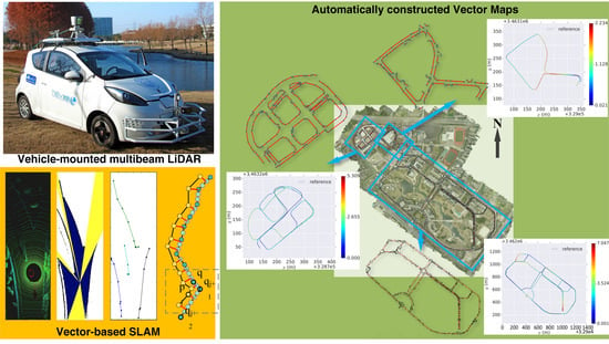
:The high-definition map (HD-map) of road structures is crucial for the safe planning and control of autonomous vehicles. However, generating and updating such maps requires intensive manual work. Simultaneous localization and mapping (SLAM) is able to automatically build and update a map of the environment. Nevertheless, there is still a lack of SLAM method for generating vector-based road structure maps. In this paper, we propose a vector-based SLAM method for the road structure mapping using vehicle-mounted multibeam LiDAR. We propose using polylines as the primary mapping element instead of grid maps or point clouds because the vector-based representation is lightweight and precise. We explored the following: (1) the extraction and vectorization of road structures based on multiframe probabilistic fusion; (2) the efficient vector-based matching between frames of road structures; (3) the loop closure and optimization based on the pose-graph; and (4) the global reconstruction of the vector map. One specific road structure, the road boundary, is taken as an example. We applied the proposed mapping method to three road scenes, ranging from hundreds of meters to over ten kilometers and the results are automatically generated vector-based road boundary maps. The average absolute pose error of the trajectory in the mapping is 1.83 m without the aid of high-precision GPS.
1. Introduction
The high-precision high-definition (HD) map of the road environment is now recognized as one of the cornerstones for autonomous driving [1,2]. The reliable mapping of road boundaries, lanes, and other road structures can significantly abbreviate the workload of an online perception system and therefore enhances the performance of autonomous driving in the complex urban environment [3]. However, the conventional method of constructing HD maps relies on massive manual labor for data postprocessing and annotation [4,5]. Therefore, it is challenging to efficiently update this manually annotated HD map timely.
Automatic mapping enabled by simultaneous localization and mapping (SLAM) has attracted the attention of many researchers. For visual SLAM, sparse feature-based methods [6] and dense methods [7] can generate a map of sparse or dense visual features for localization purposes. However, such kinds of maps cannot be directly utilized in navigation and planning. Hata and Wolf [8] exploited road information obtained from camera images, which yields a road map containing categorized road markings. Jeong et al. [9] employed a bird’s-eye view image to map the road structure. Though the lane markings and painted traffic signs are all detected and mapped using a SLAM system, the resulting map is still raster-based. Moreover, the vision-based methods suffer from limitations including, e.g., the narrow field-of-view (FOV), the short visible range and the dependence on good illumination.
In contrast, active sensing laser scanners (LiDARs) can scan the roads and facilities day and night; thus, they are preferable for mapping than vision sensors [5]. The LiDAR-based SLAM generates accurate maps represented by occupancy grids or 3D point clouds [10,11]. However, these maps are redundant and are usually of massive data volume, which are not efficient for storage and sharing. Hata and Wolf [12] employed multibeam LiDAR to detect the curbs and lane markings and generated an occupancy map of these road features. But this map was built mainly for vehicle pose estimation using Monte Carlo method. And the map is still grid-based.
Vector primitives, for example, polygons and line segments, are widely adopted as the representation of road geometry in conventional digital road maps [4]. This vectorized representation is lightweight and precise. More importantly, the vector-based map is able to hold semantic attributes such as road names and traffic rules, which are crucial for autonomous driving. However, constructing such a map relies on high-precision positioning and manual labeling. Existing SLAM methods that can produce a vector-based map were all proposed for indoor environments [13,14,15,16]. Strong assumptions of the indoor structures adopted in these studies, such as orthogonal and parallel walls, cannot be applied to road environments. As a result, there is still a lack of SLAM method that can directly generate vector-based HD road maps as demanded by autonomous driving systems.
In this paper, we propose a vector-based SLAM method for the mapping of road structures. This method is distinguished from previous studies by its vector-based map representation employed in SLAM. We explored a combined pipeline of road structure extraction and vectorization, vector-based local map matching, optimization and vector reconstruction. A vehicle-mounted multibeam LiDAR sensor, that is, the velodyne HDL-64, is used as the data source due to its 360-degree FOV, long sensing range, and high-precision measurement. We adopt a specific road structure, the road boundary, in this paper. Other structures, for example, the lanes, can be integrated with a similar method. This paper is a substantial extension of our previous paper [17]. We improved the local vector map (LVM) merging process and explored the global reconstruction of the vector map. Moreover, the road boundary map of a whole campus area was built fully automatically. This paper makes the following contributions:
- A vector-based SLAM method is explored for the automatic road structure mapping.
- A fast and precise polyline-based matching method is proposed to align vector-based local maps generated by multiframe probabilistic fusion.
- The optimization and reconstruction of local vector-based maps into a global vector map of the road structure is achieved.
2. Related Work
The automatic construction of a road structure map requires a SLAM-based solution. As being one of the most extensive research areas in the last decades, we do not attempt to give a full review of the SLAM methods. This section, however, focuses on the most relevant studies on the vector-based SLAM and distinct components that compose a SLAM system for road structure mapping, that is, the detection of road structures, the matching between frames of road structures, and the vectorization methods for road structures.
2.1. Vector-Based SLAM
Although most of the SLAM methods use points or grid maps as the mapping results [18], due to their light weight and high precision, the vector-based representation has also been explored by SLAM methods for indoor applications.
Sohn and Kim [13] presented one of the first attempts to incorporate the vector-based representation into a SLAM method. Directed line segments fitted from 2D LiDAR scans were adopted as the mapping elements. The matching between line segments was employed for loop closure and the incremental mapping were proposed by using a map merging algorithm. A similar method was proposed by Kuo et al. [14], in which SLAM was implemented using a particle filter. Both methods can generate line segments-based vector maps for the indoor environment. However, the strong indoor structure assumptions adopted in these studies, such as orthogonal and parallel walls, cannot be applied to general road environments.
Jelinek [15] proposed a vector-based mapping method based on keyframes made of edges extracted from 2D LiDAR scans. The overlapping edges of two keyframes were merged or removed according to their alignment conditions. However, this method did not implement the global optimization. Dichtl et al. [16] proposed a SLAM method that generates maps in the PolyMap format [19]. The construction of polygons from fitted lines and the polygon map merging using the BSP-tree were explored. Matching was implemented using a point-to-vector iterative closest point (ICP) method. Although the polygon-based map is suitable for representing indoor subspaces for navigation purposes, it is not able to present long and large-scale outdoor roads. Moreover, the critical global optimization in the SLAM method is also missing in this approach.
As a result, there is still a lack of a vector-based SLAM method that is suitable for automatic mapping of outdoor road structures.
2.2. Road Structure Detection
Both the vision sensor and LiDAR have been used to detect lane markings and road boundaries. In traditional vision-based methods, lane markings were detected based on the scan line or edge detection methods [20]. Recently, deep learning-based segmentation methods were proposed for extracting lanes or even road boundaries [21]. However, the performance of these methods is vulnerable to the variation of lighting conditions and imprecise measurement. Multibeam LiDAR can overcome the above shortcomings because of the 360-degree active sensing and high-precision measurement. Furthermore, geometric road structures, for example, boundaries, can be interpreted from point clouds easier than from image textures. In Hata et al. [22], curb candidates were obtained by analyzing the distance between consecutive rings, and filters were applied to remove false positives. In Hata and Wolf [8], the road marking detector employed an adapted Otsu thresholding algorithm to optimize the segmentation of point clouds based on intensity, which resulted in asphalt and road markings. In Zhang et al. [23], the spatial features of curbs in the point clouds were extracted first and then the road boundary was extracted by using curb searching. Deep learning-based methods were also proposed to detect roads and drivable areas using LiDAR data [24]. However, most of the current methods usually focus on the road boundary detection in a single frame, and thus suffer from the sparsity of point clouds far from the sensor. Therefore, a multiframe fusion is required for robust and precise road structure detection.
2.3. Road Structure Matching
The matching between frames is the basis of odometric and SLAM methods. For vision-based methods, matching is mostly reliant on the extracted features [6] or the photometric error between images [7,25]. For LiDAR-based methods, iteratively matching methods were proposed based on distance metrics between two consecutive point clouds [26,27] or between two 2D/3D grid-based local maps [28,29]. Little has been explored for directly matching between vector-based road structures.
Schreiber et al. [30] proposed a lane-marking-based matching method for vehicle localization purposes. However, the matching is between an image and a lane marking map. In Jeong et al. [9], road markings were segmented and classified first in a grid-based submap; these grid maps were then matched for detecting loops in the SLAM backend. The Chamfer matching algorithm was initially proposed by Barrow et al. [31] for finding an object in a cluttered image based on a given line drawing. Later, this method was extended to trajectory matching [32]. However, this matching method requires textual features and cannot be applied to vector-based matching.
Extended from ICP, the iterative closest line (ICL) method adopts 3D linear features to register two point clouds with the line-to-line distance metric [33]. However, this method cannot be directly applied to the matching of two frames of polylines. PL-ICP first adopts node-to-line distance metric to match between points and a polyline [34]. However, its way of establishing node-to-line correspondence may introduce error, as described in Section 3.2.2.
2.4. Road Structure Vectorization
The vector-based representation is important for the HD map to ensure its storage efficiency and usability for autonomous driving [4,35]. In traditional digital maps, the polyline is adopted as the representation for road structure [36], and such a representation always has to be vectorized from the raw nonvectorized detection, i.e., raster-based or point cloud-based. To precisely and parametrically approximate the road, studies have employed various curve models to fit the road representation. Betaille and Toledo-Moreo [37] proposed a clothoid-based road fitting method. In Jo and Sunwoo [38], a B-spline-based method was used to fit roads based on a dominant points-based B-spline curve fitting algorithm. Gwon et al. [35] proposed a piecewise polynomial curve approximation algorithm for lane-level road map generation. These studies focus on the road geometry approximation and parameterization using curve models; thus a high accuracy can be achieved. However, they only approximate the road segment in one or a few frames. To achieve global vectorization of a map, the map digitalization study still relies on a semiautomated solution [39]. As a result, the global vector-based road structure map could not be established fully automatically.
3. Approach
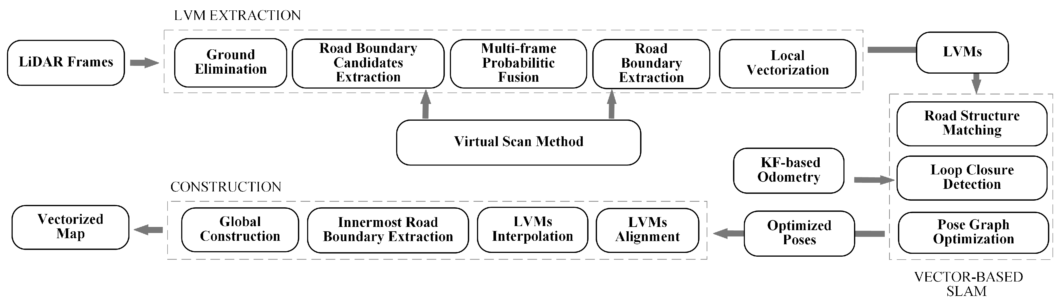
In this paper, all essential components of the automatic road boundary mapping are presented. They comprise the extraction of the local vectorized road boundary map (LVM extraction), the vector-based SLAM and the construction of the global vector map (LVM fusion). The LiDAR frames are captured by using a vehicle-mounted multibeam LiDAR sensor, that is, the velodyne HDL-64. The whole pipeline is presented in Figure 1 and will be described in detail in the following sections.
3.1. Road Boundary Extraction
Extraction of the road boundary from LiDAR scans has been studied intensively. However, the extraction in one frame or multiple directly aligned frames can be problematic because of the sparsity at a distance and the influences of dynamic objects. To overcome these problems, we adopt a probabilistic fusion method based on the 2D occupancy grid.
3.1.1. Single-Frame Road Boundary Extraction
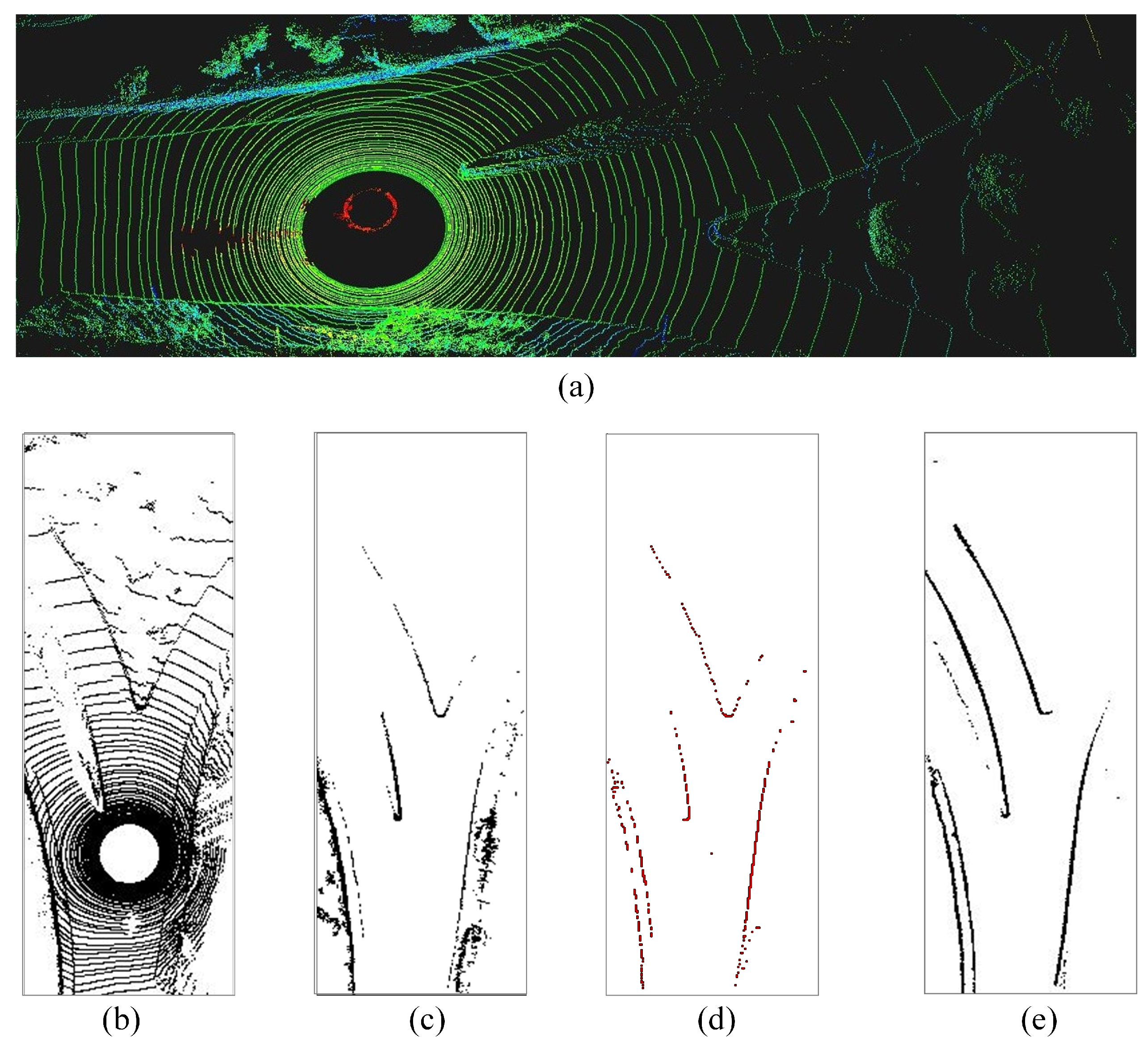
We combine the ground surface elimination and virtual scans methods to extract the road boundary in a single frame. First, we project the 3D point cloud of each frame (Figure 2a) onto a 2D grid map defined in the plane of the vehicle coordinate frame (Figure 2b). Each grid cell contains the occupancy probability and the height related information including the maximum height, minimum height, and height difference for ground elimination. Meanwhile, the grid cell can be extended to store the associated 3D points to enable the retrieval of the raw data.
Then, the ground is eliminated by obstacle segmentation, which comprises two steps: First, the average of m lowest z values of points in an downsampled grid cell is counted as . All the points in the downsampled grid cells that are higher than by a certain amount are classified as obstacle points. In the next step, we traverse each of the grid cells. The cell that contains obstacle points located within the vertical span of the vehicle is marked as an obstacle cell. After these two steps, all ground area is removed, while the grid cells representing obstacles such as road boundaries remain, as shown in Figure 2c.
In the next step, the virtual scan method [40] is applied to eliminate obstacles unrelated to the road boundary for improving accuracy and efficiency (Figure 2d). However, the extracted road boundary in one frame is sparse and can be incomplete; therefore, it should be further densified by the multiframe probabilistic fusion.
3.1.2. Multiframe Probabilistic Fusion
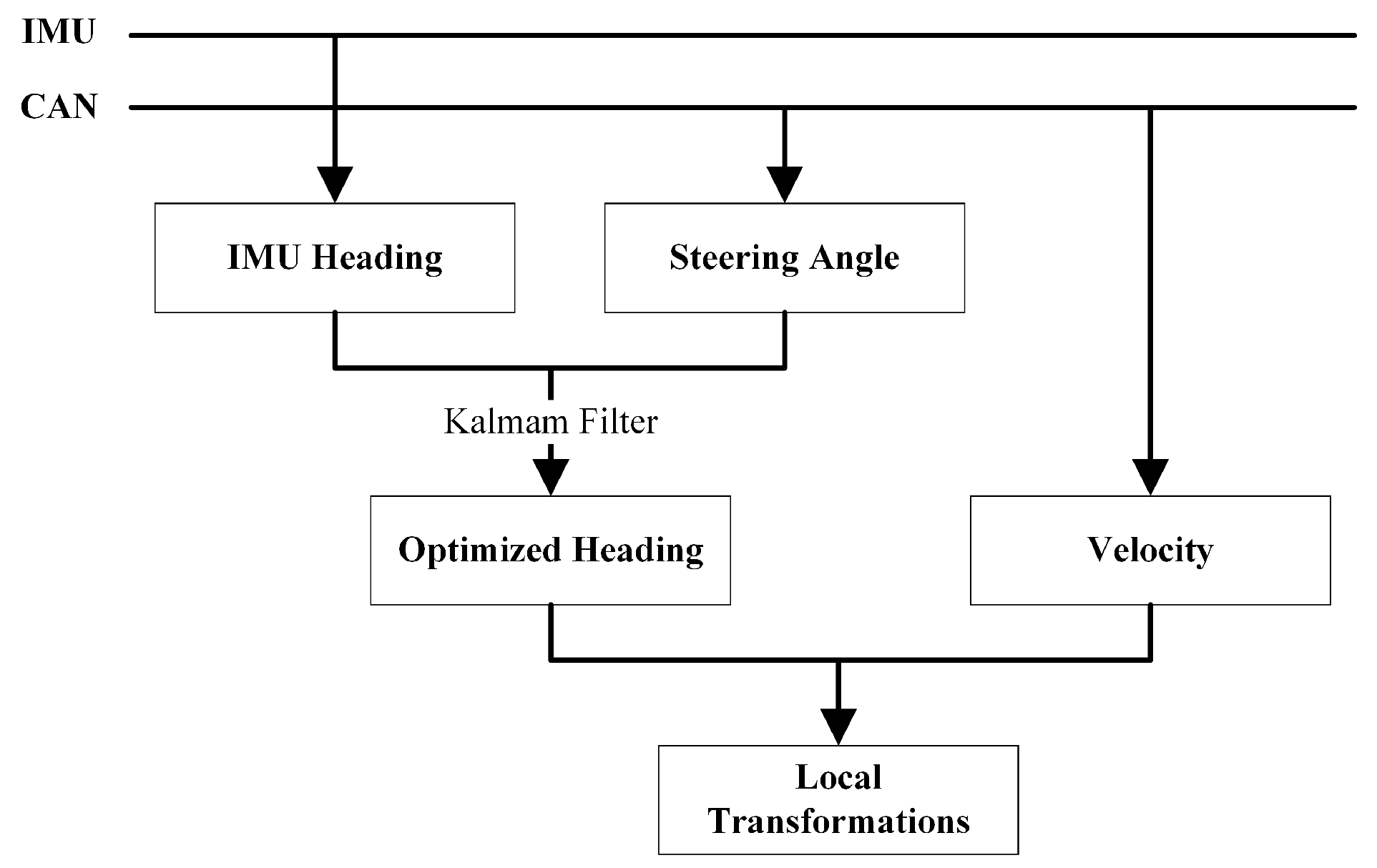
To fuse multiframes locally with high precision, we develop a reckoning system using a combination of two reckoning sources: the heading angle and velocity from the IMU and the steering angle and velocity from the vehicle (as shown in Figure 3). We first employ a Kalman filter to fuse the steering angle and heading angle into a global heading in the North-East-Down (NED) navigation coordinate frame. As a result, possible drifting of headings and accumulative errors of the steering angle are corrected. Afterward, we integrate the optimized heading with the velocity to calculate transformations of the car’s position. Because the frequency of odometry is much higher than that of LiDAR, we use the odometry to compensate for the self-motion of LiDAR and data synchronization is accomplished by timestamp interpolation.
We then fuse multiple frames of extraction results generated from the previous step by using the standard occupancy grid method. The grids are updated according to the extracted road boundaries by using odds probability maintained in each grid. As a result, the sparse extraction results can be enhanced which generate the local grid map (LGM) of road boundaries (Figure 2e). The missing road boundaries are filled and dynamic obstacles are removed, providing a good foundation for the vectorization and matching.
3.2. Vector-Based SLAM Method
In this paper, we propose to use a vectorized representation of road boundaries for SLAM because the vector-based map is favored by the HD map for its light weight and precision. We first propose a local vectorization method, which converts the road boundaries in an LGM into a polyline-based LVM. Then, an efficient road boundary matching method based on polylines is proposed to match between sequent LVMs and to detect loops. The pose-graph is then built for optimizing the whole map.
3.2.1. Local Vectorization of Road boundaries
The LGM generated in the previous step is still a grid map-based representation of road boundaries. To convert the grid map into a vector-based map, two possible routes exist: one is to first map the entire area with LGMs using a grid-based SLAM method, after which the vectorization has to deal with one global grid map; the other is to locally vectorize the LGM and use vector-based SLAM to fuse all the local vector-based maps. The former is adopted by the conventional interactive mapping process; however, the vectorization of a global grid map is known to be nontrivial due to the difficulties in tracing and arranging polylines. Moreover, mapping a large area using grid maps is also expensive. The latter approach drops the grid map early in the mapping stage and is thus lightweight. More importantly, the local vectorization of LGM is much easier than global vectorization because rays in the LiDAR scan are structured and can be utilized to trace the road boundaries. As a result, we employ the virtual scan method to locally vectorize the LGM.
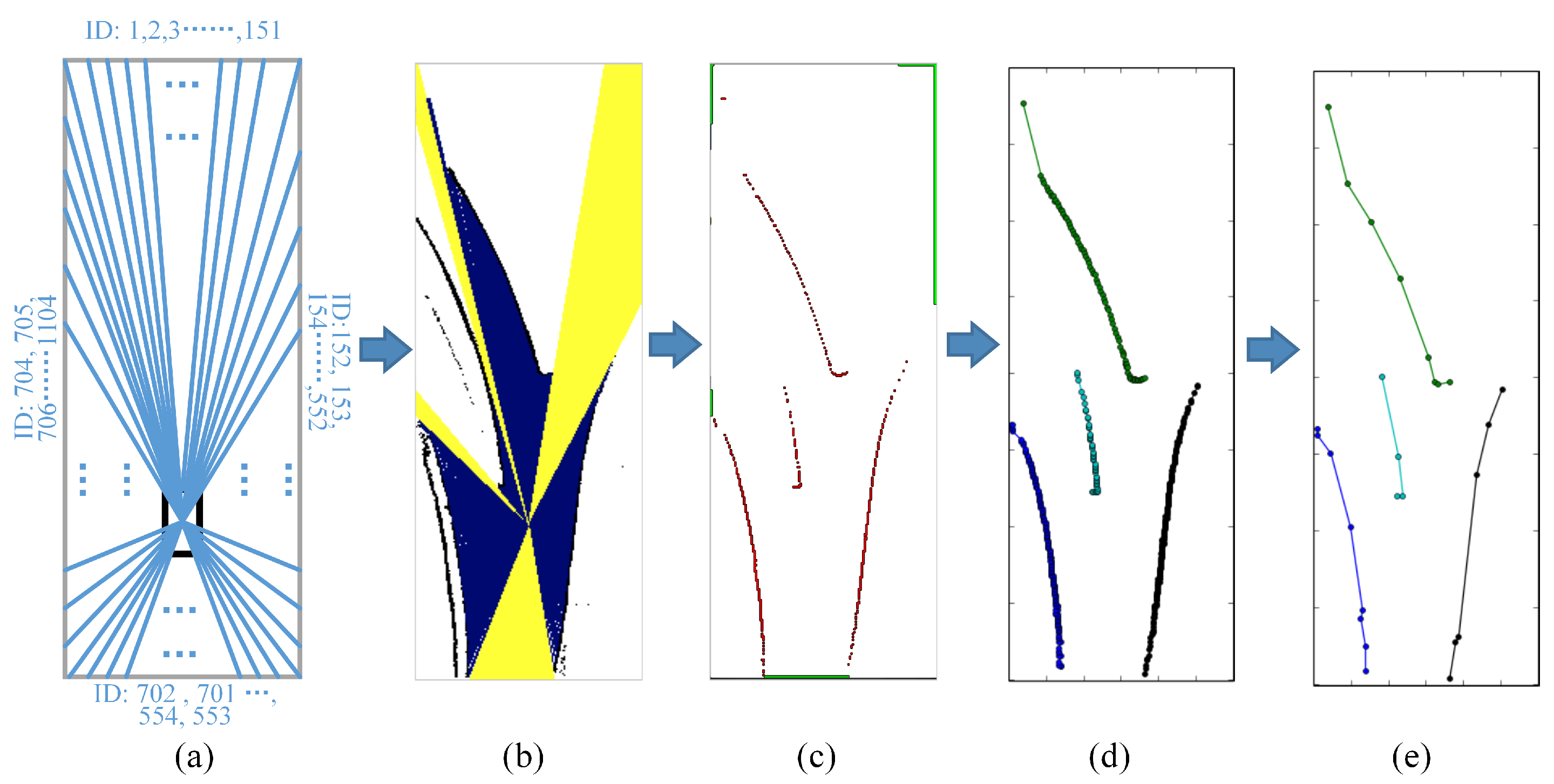
First, a set of rays is generated with the ID of each ray increasing in clockwise order (Figure 4a). Then, the points of intersection between each ray and either the grid cell representing the road boundary (hit) or the border of the grid map (miss) are calculated and considered as road boundary candidates (Figure 4b). According to the ID and the type of the intersection point, i.e., whether there is a hit at road boundaries or a miss at borders of the grid map (shown in Figure 4c by red and green, respectively) determines the clustering of the road boundary candidates into road boundaries and infinite boundaries, respectively. Moreover, within each cluster, these ordered points can be connected into a polyline according to the IDs of rays (Figure 4d), and we finally obtain a local vectorization map (LVM) of road boundaries.
Since the vectorized result can be noisy and dense due to the selected angular resolution of the virtual scan, we employ the Ramer-Douglas-Peucker algorithm [41] to optimize polylines in the LVM. The simplified representation can be reduced to merely averaging 6% of the points in the original polyline (Figure 4e), which is both lightweight and beneficial to the following matching process. For a clear description, we refer to the simplified version of LVM as simplified LVM and the original version as raw LVM.
3.2.2. Polyline-Based Matching between LVMs
To match between vectorized road boundaries, a polyline-to-polyline matching method should be employed. We formulate the distance metric of polyline pairs under the framework of ICP [42].
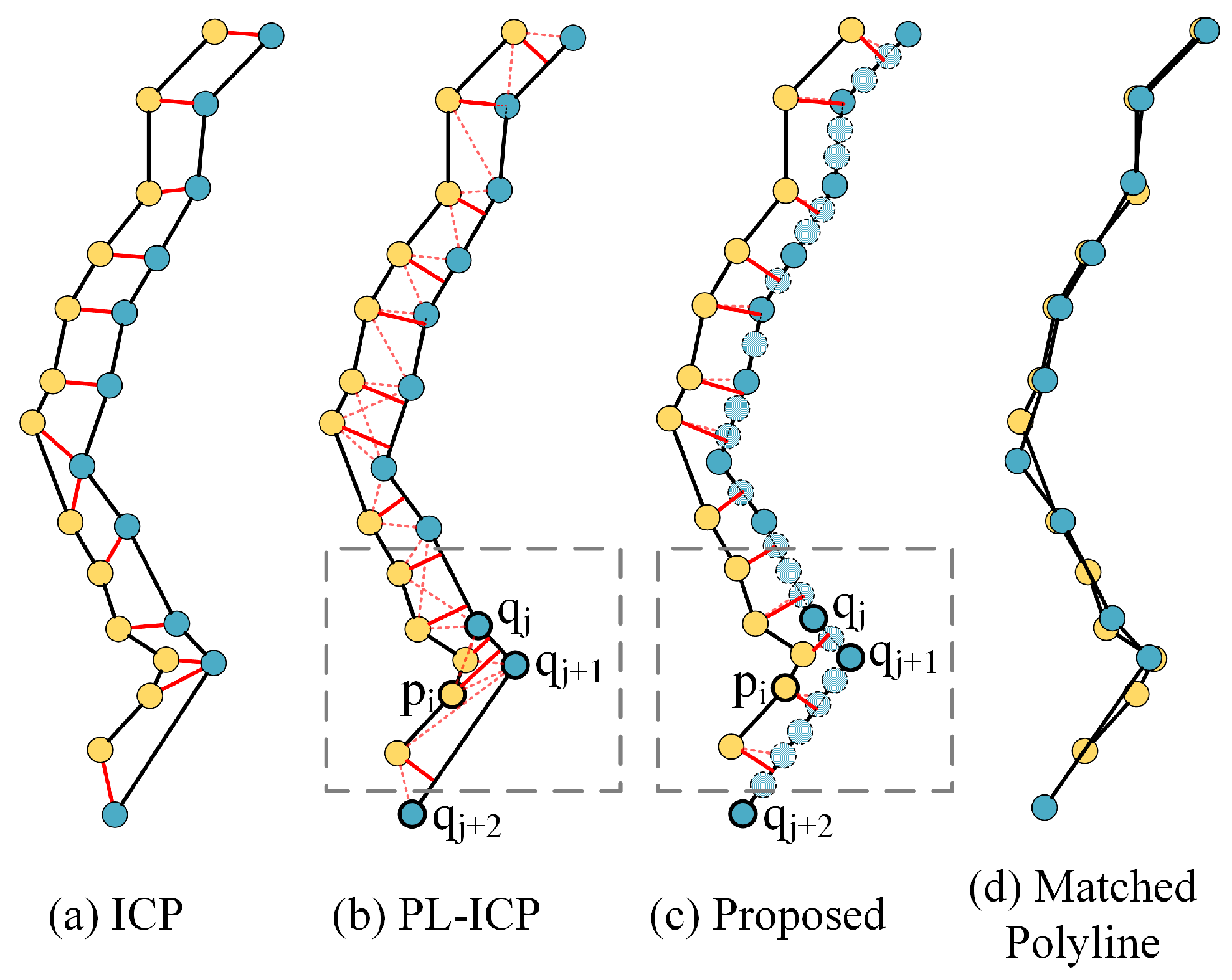
Since the exact measurement of distances between polylines can be computationally costly, we employ a fast approximation by using the node-to-line distance metric similar to PL-ICP [34]. The key difference is that we sample the nodes evenly in the referenced polyline to prevent the inaccurate node-to-line correspondence introduced by the nearest node-to-endnodes searching, as adopted by PL-ICP [34]. The comparison of various distance metrics is illustrated in Figure 5.
Figure 5a illustrates the node-to-node-based distance metric used in ICP, in which the distances between nodes do not reflect the correct distances between two polylines. Figure 5b illustrates the node-to-line-based distance metric adopted in PL-ICP. PL-ICP searches the nearest end nodes pair in the reference polyline of a node in the target polyline (as shown by the dashed red lines) to approximate the node-to-line correspondences (as shown by the solid red lines). However, erroneous correspondence is created for node because the line segment formed by the nearest end nodes pair of , , is not the nearest line segment of , which should instead be line segment . This is especially common in our case because the nodes in a simplified polyline are sparse.
To overcome this problem, we propose to first sample the reference polyline evenly, as shown by the cyan nodes in Figure 5c. Then, the nearest node in the sampled reference polyline is founded for each of the nodes in the target polyline (as shown by the dashed red lines); such correspondences are finally used to correctly establish the node-to-line correspondence (as shown by the solid red lines). The node is therefore correctly corresponded to line segment as shown in Figure 5c.
Based on the correspondence between polylines, the optimization function is similar to that of PL-ICP:
where R and T are rotation and translation between the unregistered and the referenced polyline, respectively. Assuming that the tuple <,,> is the found node-to-line correspondence in each step, point from the unregistered polyline is matched to segment - from the referenced polyline. is the normal of the line segment represented by the node pair [, ] in the referenced polyline. Finally, the iterative optimization matches the two polylines as shown in Figure 5d. It should be noted that the sampled nodes in the proposed method are not included in the optimization; thus, not much computational burden is introduced.
Moreover, we will show later in Section 4.1.1 that the simplified-LVM-based matching converges faster than raw-LVM-based matching and yields better precision for matching.
3.2.3. Loop Detection and Optimization
We use the KF-based odometry to estimate whether the vehicle revisits the same place as before, and we use the threshold of the matching error between LVMs to detect potential loops. The [43] package is adopted to construct a pose graph for the optimization. The least square problem can then be solved by minimization of the following objective function:
where represents the pose of the vehicle at time t. The function is the state transition model for two poses. The and represent the constraints from odometry and vector-based matching. The covariances of odometry and vector-based matching are denoted as and , respectively.
3.3. LVM Fusion by Reconstruction
The optimized LVMs should be fused into a consistent vector-based representation. In our previous paper [17], the LVMs are concatenated frame-by-frame. However, we found the method is vulnerable to noise and positioning errors. Moreover, the global structure of the map was not taken into consideration, which is crucial for the vectorization of complex intersections. As a result, we proposed a global LVM reconstruction method: First, the LVMs are fused without concatenation. A probe-based sampling method is then employed to sample the fused road boundaries. Finally, a reconstruction method is employed to globally reconstruct the vector map from sampled LVMs.
3.3.1. Probe-Based Sampling
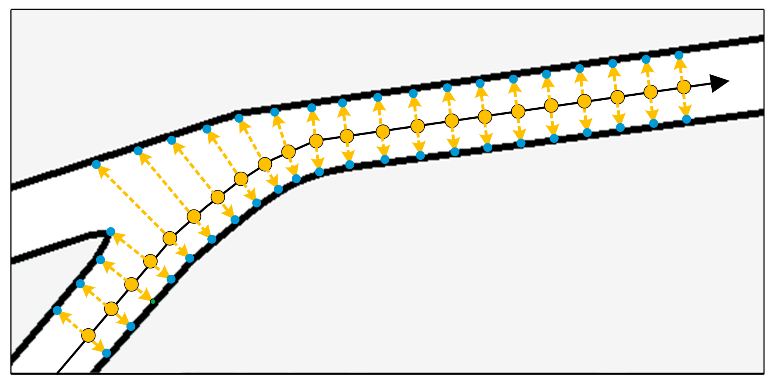
The fused LVMs may suffer from ghost effects due to the remaining error of the optimized pose, which prohibits the accurate vectorization. To filter out the ghost effects, we utilize the trajectories of the vehicle and employ “probing” of the innermost road boundaries along the trajectory. As shown in Figure 6, along a trajectory of the vehicle, two “probing” rays are generated along the normal direction of the interpolated trajectory. The closet intersecting points on the polyline representing road boundaries are selected as the filtered road boundaries. As required by the following reconstruction method, we densely sampled the road boundary and generate a uniform innermost road boundary point set.
3.3.2. Fusion by Reconstruction
A shape reconstruction method, the optimal transport curve reconstruction (OTCR), is employed to reconstruct the final vector map [44]. The OTCR views shape reconstruction and simplification as a transport problem between measures, where the input point set is considered as a Dirac measure and the reconstructed simplicial complex is seen as the support of a piecewise uniform measure [44]. Based on Delauney triangulation and following edge collapsing and vertex relocation, this method can preserve the structure of the densely sampled road boundaries and treat noise and outliers in a unified fashion.
4. Experimental Analysis
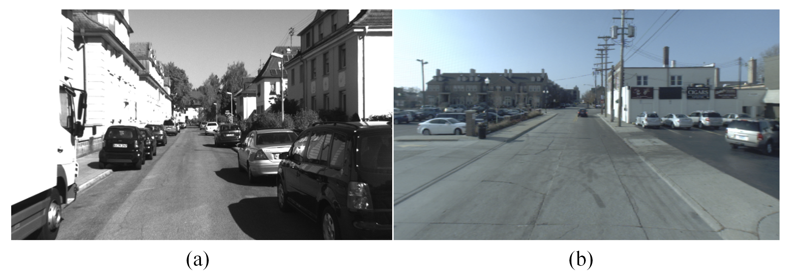
In this paper, all the experimental datasets were captured at Jiading campus of Tongji University, since the road boundary in many openly available LiDAR datasets, such as the KITTI [45] and Ford Campus [46] datasets, are either colluded or simply missing (as shown in Figure 7).
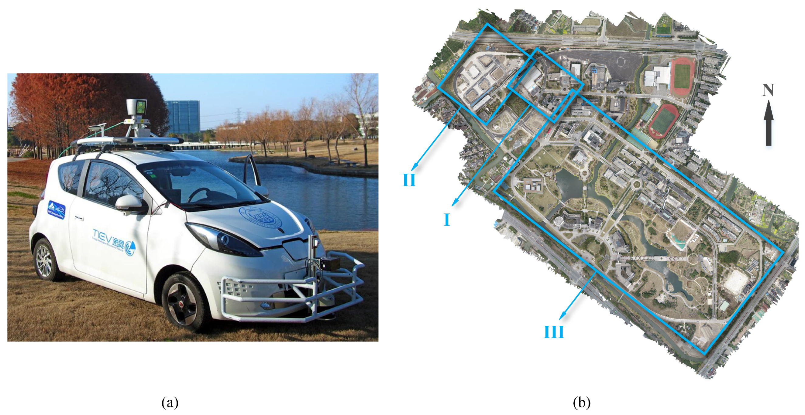
We selected three areas of the campus for the experiments, shown by I, II and III boxes in Figure 8b). The lengths of the mapped road range from several hundred meters (area I—a single loop) to over 10 km (area III—the major part of the campus). The vector-based mapping results for each area are shown and quantitatively compared with the ground truth using the EVO tool [47]. The brief results of road boundary extraction and matching in the first experiment are provided; for more detailed results, please refer to our previous paper [17].
All the datasets are captured using our TiEV autonomous driving platform (cs1.tongji.edu.cn/tiev) (Figure 8a). The platform-equipped sensors include a Velodyne HDL-64 and an integrated INS system OxTS RT2000 with RTKGPS. However, the captured high-precision positioning result is only used as the ground truth and to initially set the direction and position of the vehicle at the start of mapping. The frequency of the LiDAR scan is 10 Hz, and the velocity of the vehicle during data capture ranged from 10 to 20 km/h.
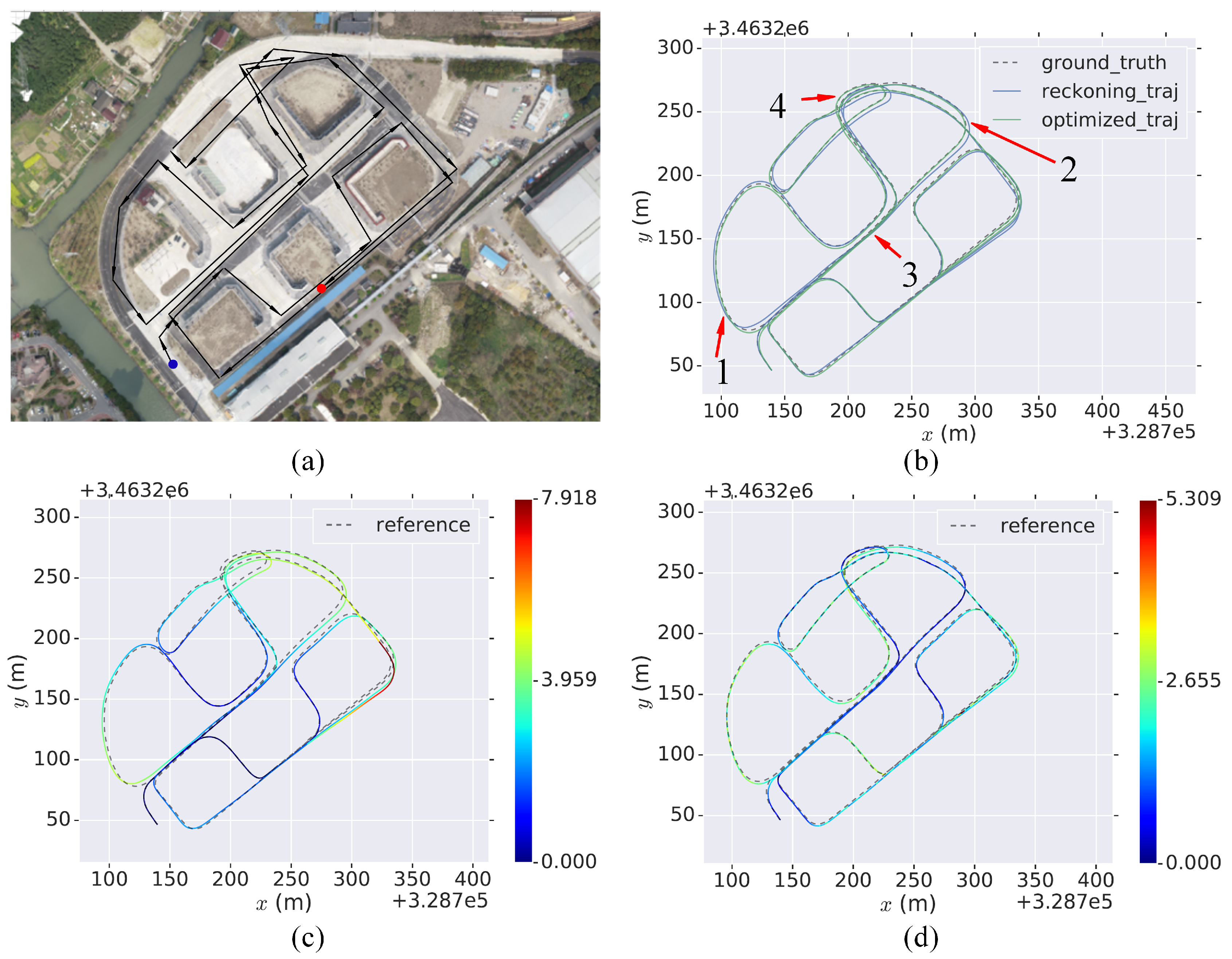
4.1. Experiment I—Road Boundary Mapping of a Loop Road
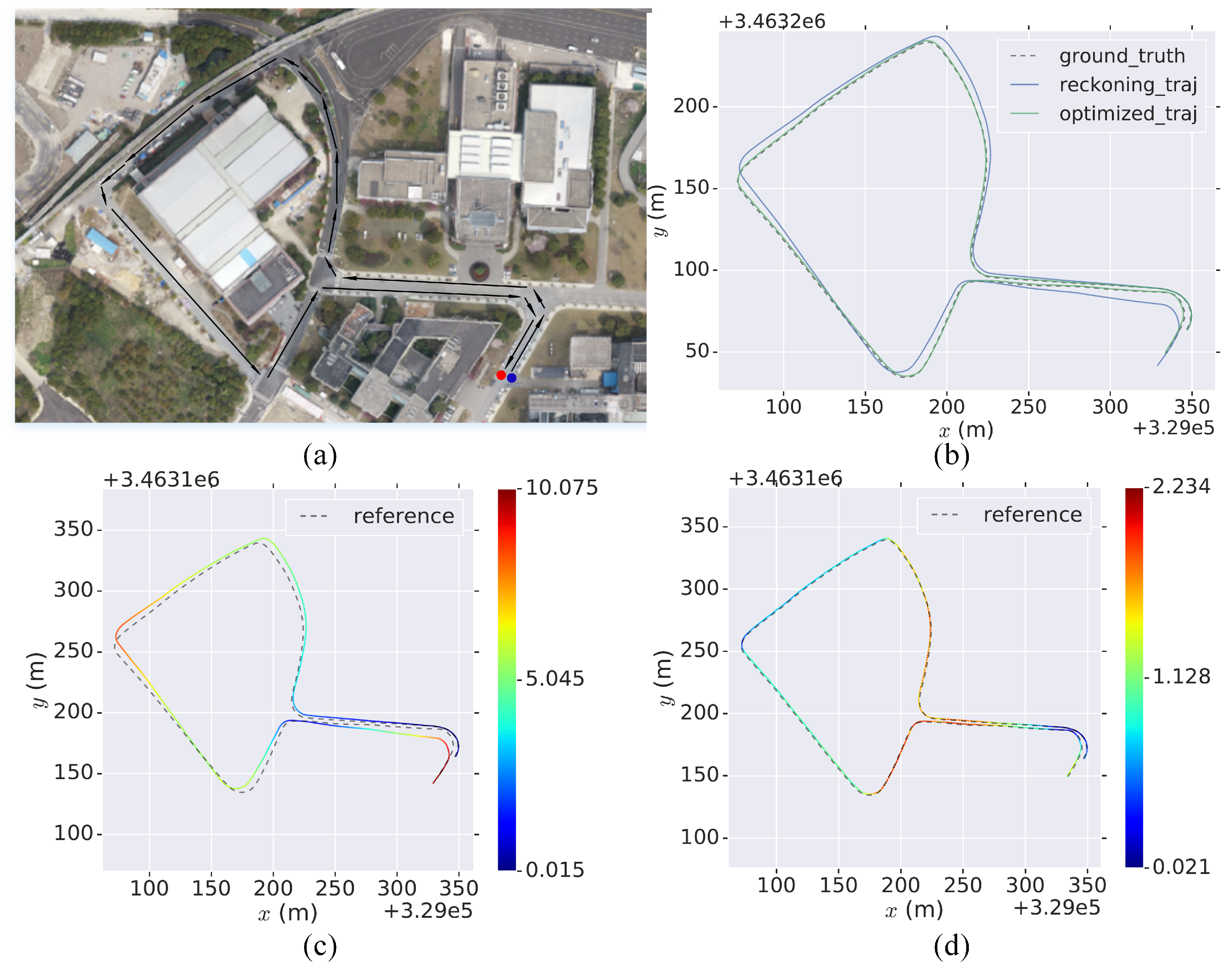
In this experiment, a simple loop road as shown in Figure 10a is adopted. Its total length is 860 m with 5 major intersections and several roadside branch paths. The purpose of this experiment is to validate the effectiveness of the proposed vector-based SLAM system, including road boundary extraction, matching and loop detection, and optimization. We captured the data in the evening without much intervention from dynamic objects.
4.1.1. Road Boundary Extraction and Matching
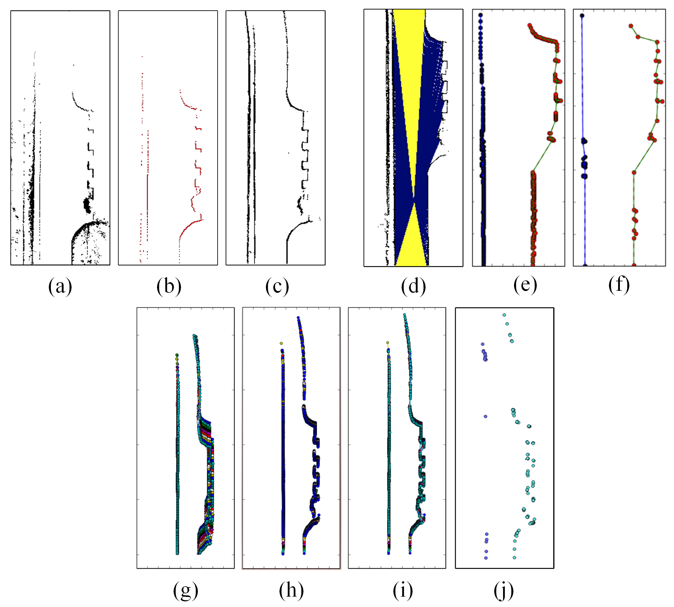
Based on the performance of our dead-reckoning system, we probabilistically fused 280 consequent frames to build the LGM. The dimension of the LGM for fusion is defined as 401 by 151 with a grid resolution of 20 cm, which is derived from requirements of TiEV’s planning module and can be adjusted when needed. Figure 9 illustrates the LGM and LVM extraction and LVM-based matching processes.
Figure 9a–c show the road boundary extraction in multiple frames. Figure 9a shows the projected point cloud after ground elimination. Figure 9b shows the extracted road boundary in one frame. Figure 9c shows the probabilistically fused LGM, which is a complete and dense representation of road boundaries.
Figure 9d–f show the LVM extraction based on the vectorization of an LGM. Figure 9d shows the classification of the rays of a virtual scan resulting an ordered clustering of road boundaries. In Figure 9e, the ordered points belonging to a sector of the road boundaries are connected to realize the initial vectorization. We simplified the initial vectorization, the raw-LVM, by using the Ramer-Douglas-Peucker method and produced the simplified-LVM (Figure 9f), which is accurate as well as efficient for storage and processing.
Figure 9g–j demonstrates the results of matching. The results of ICP (based on projected point clouds) and our method (vector-based matching of LVMs) are compared. In Figure 9g, the original 10 frames for matching are shown. The matching result with ICP is shown in Figure 9h, where misalignments are easily visible as “thick” point clouds. The matching with raw-LVMs and simplified-LVMs with the proposed matching method are shown in Figure 9i,j, respectively. Both results are superior to ICP and the latter obtains the best results with the points that are all overlapped (Figure 9j).
The quantitative evaluation of the performance of matching is shown in Table 1. The mean absolute errors and time costs indicate the matching with simplified-LVMs outperforms raw-LVM-based matching and ICP in both accuracy and efficiency because of its lightweight and less noisy polyline-based representation.
4.1.2. Evaluation of the Trajectory
The comparisons of the ground truth, reckoning-based trajectory, and optimized trajectory are shown in Figure 10b. The quantitative evaluation of the trajectory without and with optimization are shown in Figure 10c,d. In Figure 10c, noticeable misalignment can be observed between the reckoning-based trajectory and the ground truth. Based on the detected loop closure through the matching of LVMs, the optimization effectively corrected the cumulative error (as shown in Figure 10d). The comparison of the error statistics of the two results are given in Table 2.
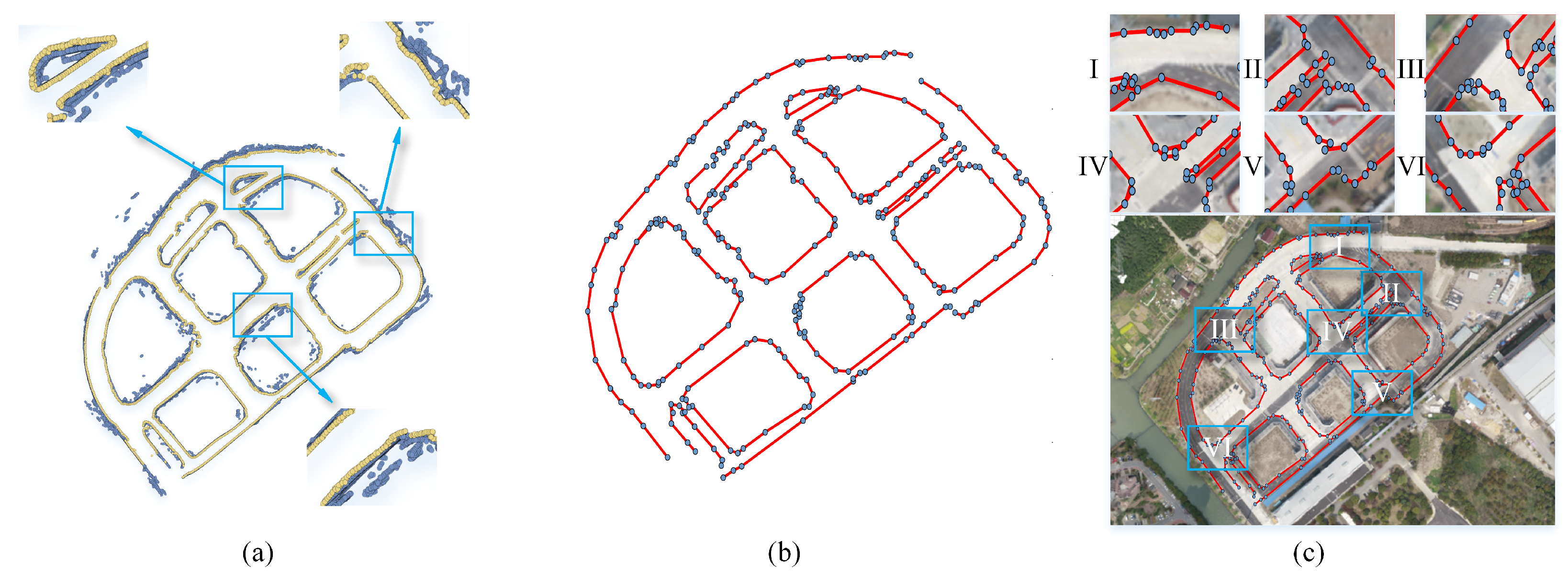
4.1.3. Evaluation of the Map
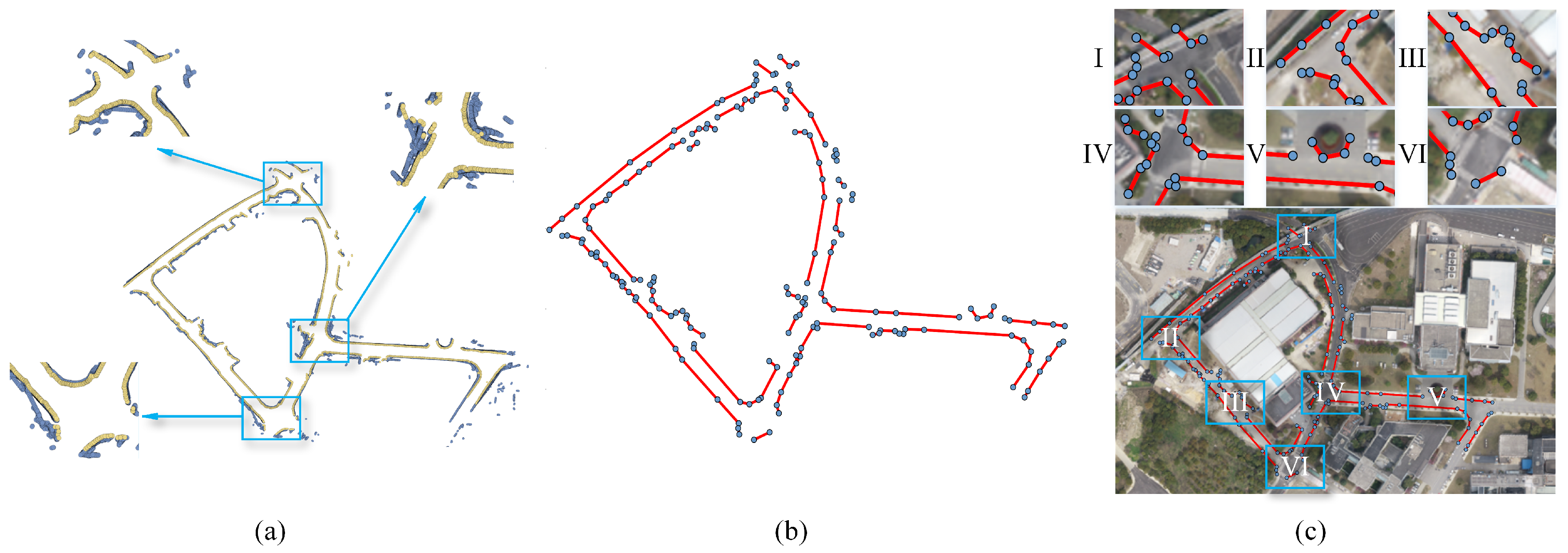
Based on the optimized trajectory, all the LVMs are aligned to construct the global vector map. In Figure 11a, the yellow points represent the extracted innermost road boundary points by the probe-based sampling method. Figure 11b shows the reconstructed global vector map from the innermost road boundary points. To intuitively exhibit the mapping result, the vector map is overlaid on the aerial image of the mapped area (Figure 11c). This result shows that the vectorized map retains the structure of the road boundary in a vectorized form, which aligns well with the actual road boundary. Figure 11c-I, II, and VI show successfully mapped intersections; all the road boundaries along the trajectory are mapped except for those far away from the trajectory. Figure 11c-I presents an intersection nearby an overbridge, and the ground road boundary is mapped. In Figure 11c-III, the road boundary near an entrance of a building is shown. Since the entrance is not separated from the road by curbs, the mapped road boundary extended to the layout of the building. Figure 11c-IV shows a complex intersection with multiple lanes and vegetated areas. The mapped road boundary twisted slightly on the border of the vegetation on the left. The cause is the uneven distribution of the vegetation. Figure 11c-V shows a roundabout along the road, and the boundary along the trajectory is mapped correctly.
4.2. Experiment II—Road Boundary Mapping of the IV Evaluation Field
We then applied our method to a more complex road environment, the Intelligent Vehicle (IV) Evaluation field of Tongji University. The data collecting path is approximately 2 km in length, passing through all road segments, including 3 cross-intersections and 8 T-junctions (as shown in Figure 12a). The evaluation field was nearly free of dynamic intervening aspects during the data capture and road lying in the field is not yet completed.
4.2.1. Evaluation of the Trajectory
The comparison between the reckoning-based trajectory and the optimized trajectory is shown in Figure 12b. The absolute position errors of both trajectories are shown in Figure 12c,d. It can be seen from 1 and 3 in Figure 12b that the reckoning system is accurate in straight and gently curved roads of such a scene. Moreover, 2 and 4 show the optimization corrected the accumulated error by utilizing multiple loops detected during the path. However, in the optimized path, the error at point 2 is significantly lower than that at point 1, as indicated in Figure 12d. This occurred because the vehicle passed multiple times near 2, which resulted in extra loops. The comparison of the error statistics of the two results is given in Table 3.
4.2.2. Evaluation of the Map
Figure 13a shows the aligned global road boundary points and the extracted innermost points. Figure 13b is the result of vector-based mapping. Detailed examples can be found in Figure 13c. In Figure 13c-I, the asphalt road merged to the road under construction (shown as the light gray area); therefore, no separating boundary can be mapped. The same case can be found in Figure 13c-VI. In Figure 13c-II, all the road boundaries, even the narrow pedestrian path, are mapped. In Figure 13c-III, IV and V, zigzag boundaries are present on the road corners. This result is due to the alignment errors in some corners, as seen by thick yellow points in blue boxes in Figure 13a. The reason could be the multiple reflections from glass and uncorrected matching errors.
4.3. Experiment III—Road Boundary Mapping of the Campus
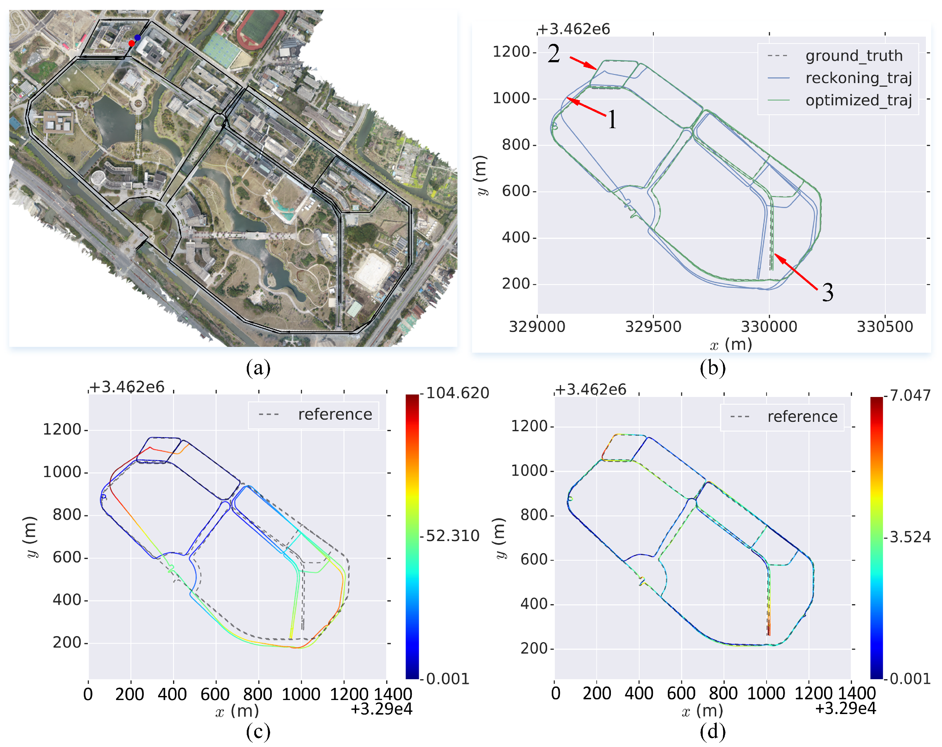
4.3.1. Evaluation of the Trajectory
To verify the performance of our method with large-scale data, we applied our method to the Jiading campus of Tongji University, with a total path length of 11 km and coverage of 1200 by 980 m (Figure 14a). The campus roads inevitably contain traffic and pedestrians, which impose great challenges on the mapping.
Figure 14b is the comparison of the ground truth, reckoning-based and optimized trajectories. It can be seen that the deviation between the reckoning-based trajectory and ground truth is large, especially at point 1 and 2. This deviation is also depicted by the absolute positioning error of the reckoning-based trajectory (Figure 14c). The largest deviation is approximately 100 m, caused by the accumulated error of the heading.
In Figure 14d, the optimization significantly reduces the error. At point 1 shown in Figure 14b, the error is reduced to approximately 2 m. However, the positioning errors of the optimized trajectory at point 2 and point 3 are still large, which range from approximately 5 to 7 m. This result is due to the lack of revisiting, e.g., point 3 is a temporarily blocked road; thus, no loop can be found at the end. The comparison of the error statistics of the two results is given in Table 4.
4.3.2. Evaluation of the Map
The constructed global map of the campus is shown in Figure 15. As shown in Figure 15a, the innermost road boundary points (yellow) effectively tracked the structure of the noisy road measurements, especially in two complex roundabouts. The entire reconstructed vector map is shown in Figure 15b. From Figure 15c, it can be seen that most of the road structures are mapped correctly. In Figure 15c-I, small gaps on the road boundary are formed by the presence of branch paths. In Figure 15c-II, a small portion of the boundary of the roundabout is left open, which is due to having missed the data collection, as shown by the path in Figure 14a. Figure 15c-III and IV depict examples of completely mapped roads, while Figure 15c-V and VI show the complex roundabout and intersection with artificial blockages. However, the proposed method could still map such areas automatically.
5. Concluding Remarks
The vectorized HD map of road structures is crucial for autonomous driving systems. However, building and updating such a map manually or semiautomatically is expensive and, as such, has become an obstacle for the application of autonomous vehicles. This paper explored a fully automated work flow of mapping the road boundary in a vector-based form using multibeam LiDAR and IMU data. The local road boundary map is extracted from a multiple-frame fusion and is vectorized early in the work flow. The polyline-based matching method is proposed to match between local vector maps and to detect loops. The aligned local vector maps are finally sampled and are globally reconstructed to yield a global vector map. The experiments carried out in various-sized road environments prove the effectiveness of the proposed method. However, the results presented are still not perfect. For example, implementing purely vector-based matching tends to yield large errors in straight and smooth roads due to the lack of geometric features. Therefore, a reliable reckoning system is indispensable. Moreover, large debris on some rural roads may lead to false road boundaries in the mapping result, which need to be further eliminated by counting the length of the boundaries. Furthermore, the reconstructed vector map presents many discontinuities due to the missed road boundaries. Such a result may be utilized to diagnose the pavements and curbs in road engineering [48]. However, for mapping, many of these cases can be deduced and fixed by an experienced human mapper, which, at present, cannot be interpreted by the proposed algorithm.
Future work includes the improvement of the matching accuracy in a feature-less road environment by incorporating more road structure information such as lane markings. In addition, the semantic enrichment of the road boundaries and the semantic-aided gap fixing require further explorations.
Author Contributions
Conceptualization, J.Z.; methodology, J.Z. and X.H.; software, X.H.; validation, X.H. and J.L.; resources, C.Y. and L.X.; writing review and editing, T.F.; and supervision, J.Z.
Funding
This work is supported by the National Key Research and Development Program of China (No. 2017YFA0603100, 2018YFB0105103 and 2018YFB0505400), the National Natural Science Foundation of China (No. U1764261, 41801335, and 41871370), the Shanghai Science and Technology Development Foundation (No. 17DZ1100202 and 16DZ1100701) and the Fundamental Research Funds for the Central Universities (No. 22120180095).
Acknowledgments
We thank Enwei Zhang and Hongtu Zhou for helping capture the data and thank Sébastien Loriot and Pierre Alliezfor for fixing the bugs in the OTCR package of CGAL.
Conflicts of Interest
The authors declare no conflict of interest.
References
- Seif, H.G.; Hu, X. Autonomous Driving in the iCity—HD Maps as a Key Challenge of the Automotive Industry. Engineering 2016, 2, 159–162. [Google Scholar] [CrossRef]
- Joshi, A.; James, M.R. Generation of Accurate Lane-Level Maps from Coarse Prior Maps and Lidar. IEEE Intell. Transp. Syst. Mag. 2015, 7, 19–29. [Google Scholar] [CrossRef]
- Zhao, J.; Ye, C.; Wu, Y.; Guan, L.; Cai, L.; Sun, L.; Yang, T.; He, X.; Li, J.; Ding, Y.; et al. TiEV: The Tongji Intelligent Electric Vehicle in the Intelligent Vehicle Future Challenge of China. In Proceedings of the IEEE International Conference on Intelligent Transportation Systems (ITSC), Maui, HI, USA, 4–7 November 2018; pp. 1303–1309. [Google Scholar]
- Bender, P.; Ziegler, J.; Stiller, C. Lanelets: Efficient map representation for autonomous driving. In Proceedings of the IEEE Intelligent Vehicles Symposium (IV), Ypsilanti, MI, USA, 8–11 June 2014; pp. 420–425. [Google Scholar]
- Aeberhard, M.; Rauch, S.; Bahram, M.; Tanzmeister, G. Experience, Results and Lessons Learned from Automated Driving on Germany’s Highways. IEEE Intell. Transp. Syst. Mag. 2015, 7, 42–57. [Google Scholar] [CrossRef]
- Mur-Artal, R.; Montiel, J.M.M.; Tardós, J.D. ORB-SLAM: A Versatile and Accurate Monocular SLAM System. IEEE Trans. Robot. 2017, 31, 1147–1163. [Google Scholar] [CrossRef]
- Engel, J.; Schöps, T.; Cremers, D. LSD-SLAM: Large-scale direct monocular SLAM. In Proceedings of the European Conference on Computer Vision, Zurich, Switzerland, 6–12 September 2014; pp. 834–849. [Google Scholar]
- Hata, A.; Wolf, D. Road marking detection using LIDAR reflective intensity data and its application to vehicle localization. In Proceedings of the IEEE International Conference on Intelligent Transportation Systems, Qingdao, China, 8–11 October 2014; pp. 584–589. [Google Scholar]
- Jeong, J.; Cho, Y.; Kim, A. Road-SLAM: Road marking based SLAM with lane-level accuracy. In Proceedings of the IEEE Intelligent Vehicles Symposium (IV), Redondo Beach, CA, USA, 11–14 June 2017; pp. 1736–1743. [Google Scholar]
- Zhang, J.; Singh, S. LOAM: Lidar Odometry and Mapping in Real-time. In Proceedings of the Robotics: Science and Systems, Berkeley, CA, USA, 12–16 July 2014. [Google Scholar] [CrossRef]
- Hess, W.; Kohler, D.; Rapp, H.; Andor, D. Real-time loop closure in 2D LIDAR SLAM. In Proceedings of the IEEE International Conference on Robotics and Automation (ICRA), Stockholm, Sweeden, 16–21 May 2016; pp. 1271–1278. [Google Scholar]
- Hata, A.Y.; Wolf, D.F. Feature Detection for Vehicle Localization in Urban Environments Using a Multilayer LIDAR. IEEE Trans. Intell. Transp. Syst. 2016, 17, 420–429. [Google Scholar] [CrossRef]
- Sohn, H.J.; Kim. VecSLAM: An Efficient Vector-Based SLAM Algorithm for Indoor Environments. J. Intell. Robot. Syst. 2009, 56, 301–318. [Google Scholar] [CrossRef]
- Kuo, B.W.; Chang, H.H.; Chen, Y.C.; Huang, S.Y. A Light-and-Fast SLAM Algorithm for Robots in Indoor Environments Using Line Segment Map. J. Robot. 2011, 2011, 12. [Google Scholar] [CrossRef]
- Jelinek, A. Vector maps in mobile robotics. Acta Polytech. Ctu Proc. 2015, 2, 22–28. [Google Scholar] [CrossRef]
- Dichtl, J.; Le, X.S.; Lozenguez, G.; Fabresse, L.; Bouraqadi, N. PolySLAM: A 2D Polygon-based SLAM Algorithm. In Proceedings of the IEEE International Conference on Autonomous Robot Systems and Competitions (ICARSC), Porto-Gondomar, Portugal, 24–26 April 2019; pp. 1–6. [Google Scholar]
- He, X.; Zhao, J.; Sun, L.; Huang, Y.; Zhang, X.; Li, J.; Ye, C. Automatic Vector-based Road Structure Mapping Using Multi-beam LiDAR. In Proceedings of the IEEE International Conference on Intelligent Transportation Systems (ITSC), Auckland, New Zealand, 27–30 October 2018; pp. 417–422. [Google Scholar]
- Cadena, C.; Carlone, L.; Carrillo, H.; Latif, Y.; Scaramuzza, D.; Neira, J.; Reid, I.; Leonard, J.J. Past, Present, and Future of Simultaneous Localization and Mapping: Toward the Robust-Perception Age. IEEE Trans. Robot. 2016, 32, 1309–1332. [Google Scholar] [CrossRef]
- Dichtl, J.; Luc, F. PolyMap: A 2D Polygon-Based Map Format for Multi-robot Autonomous Indoor Localization and Mapping. In Intelligent Robotics and Applications; Springer: Cham, Switzerland, 2018; pp. 120–131. [Google Scholar]
- Borkar, A.; Hayes, M.; Smith, M.T. A Novel Lane Detection System With Efficient Ground Truth Generation. IEEE Trans. Intell. Transp. Syst. 2012, 13, 365–374. [Google Scholar] [CrossRef]
- Badrinarayanan, V.; Kendall, A.; Cipolla, R. SegNet: A Deep Convolutional Encoder-Decoder Architecture for Image Segmentation. IEEE Trans. Pattern Anal. Mach. Intell. 2017, 39, 2481–2495. [Google Scholar] [CrossRef]
- Hata, A.Y.; Osorio, F.S.; Wolf, D.F. Robust curb detection and vehicle localization in urban environments. In Proceedings of the IEEE Intelligent Vehicles Symposium (IV), Ypsilanti, MI, USA, 8–11 June 2014; pp. 1257–1262. [Google Scholar]
- Zhang, Y.; Wang, J.; Wang, X.; Dolan, J.M. Road-Segmentation-Based Curb Detection Method for Self-Driving via a 3D-LiDAR Sensor. IEEE Trans. Intell. Transp. Syst. 2018, 19, 3981–3991. [Google Scholar] [CrossRef]
- Caltagirone, L.; Scheidegger, S.; Svensson, L.; Wahde, M. Fast LIDAR-based road detection using fully convolutional neural networks. In Proceedings of the IEEE Intelligent Vehicles Symposium (IV), Redondo Beach, CA, USA, 11–14 June 2017; pp. 1019–1024. [Google Scholar] [CrossRef]
- Engel, J.; Koltun, V.; Cremers, D. Direct Sparse Odometry. IEEE Trans. Pattern Anal. Mach. Intell. 2016, 40, 611–625. [Google Scholar] [CrossRef]
- Olson, E.B. Real-time correlative scan matching. In Proceedings of the IEEE International Conference on Robotics and Automation (ICRA), Kobe, Japan, 12–17 May 2009; pp. 1233–1239. [Google Scholar]
- Rusinkiewicz, S.; Levoy, M. Efficient variants of the ICP algorithm. In Proceedings of the Third International Conference on 3-D Digital Imaging and Modeling, Quebec City, QC, Canada, 28 May–1 June 2001; pp. 145–152. [Google Scholar]
- Hahnel, D.; Burgard, W.; Fox, D.; Thrun, S. A highly efficient FastSLAM algorithm for generating cyclic maps of large-scale environments from raw laser range measurements. In Proceedings of the IEEE/RSJ International Conference on Intelligent Robots and Systems (IROS), Las Vegas, NV, USA, 27–31 October 2003; Volume 1, pp. 206–211. [Google Scholar]
- Biber, P.; Straßer, W. The normal distributions transform: A new approach to laser scan matching. In Proceedings of the IEEE/RSJ International Conference on Intelligent Robots and Systems (IROS), Las Vegas, NV, USA, 27–31 October 2003; Volume 3, pp. 2743–2748. [Google Scholar]
- Schreiber, M.; Knöppel, C.; Franke, U. LaneLoc: Lane marking based localization using highly accurate maps. In Proceedings of the IEEE Intelligent Vehicles Symposium (IV), Gold Coast, Australia, 23–26 June 2013; pp. 449–454. [Google Scholar]
- Barrow, H.G.; Tenenbaum, J.M.; Bolles, R.C.; Wolf, H.C. Parametric Correspondence and Chamfer Matching: Two New Techniques for Image Matching. Proc. Int. Jt. Conf. Artif. Intell. 1977, 2, 1961. [Google Scholar]
- Floros, G.; Zander, B.V.D.; Leibe, B. OpenStreetSLAM: Global vehicle localization using OpenStreetMaps. In Proceedings of the IEEE International Conference on Robotics and Automation (ICRA), Karlsruhe, Germany, 6–10 May 2013; pp. 1054–1059. [Google Scholar]
- Alshawa, M. lCL: Iterative closest line A novel point cloud registration algorithm based on linear features. Ekscentar 2007, 10, 53–59. [Google Scholar]
- Censi, A. An ICP variant using a point-to-line metric. In Proceedings of the IEEE International Conference on Robotics and Automation (ICRA), Pasadena, CA, USA, 19–23 May 2008; pp. 19–25. [Google Scholar]
- Gwon, G.P.; Hur, W.S.; Kim, S.W.; Seo, S.W. Generation of a Precise and Efficient Lane-Level Road Map for Intelligent Vehicle Systems. IEEE Trans. Veh. Technol. 2017, 66, 4517–4533. [Google Scholar] [CrossRef]
- Haklay, M.; Weber, P. Openstreetmap: User-generated street maps. IEEE Pervasive Comput. 2008, 7, 12–18. [Google Scholar] [CrossRef]
- Betaille, D.; Toledo-Moreo, R. Creating Enhanced Maps for Lane-Level Vehicle Navigation. IEEE Trans. Intell. Transp. Syst. 2010, 11, 786–798. [Google Scholar] [CrossRef]
- Jo, K.; Sunwoo, M. Generation of a precise roadway map for autonomous cars. IEEE Trans. Intell. Transp. Syst. 2014, 15, 925–937. [Google Scholar] [CrossRef]
- Foroutan, M.; Zimbelman, J. Semi-automatic mapping of linear-trending bedforms using Self-Organizing Maps algorithm. Geomorphology 2017, 293, 156–166. [Google Scholar] [CrossRef]
- Montemerlo, M.; Becker, J.; Bhat, S.; Dahlkamp, H.; Dolgov, D.; Ettinger, S.; Haehnel, D.; Hilden, T.; Hoffmann, G.; Huhnke, B., Jr. The Stanford entry in the Urban Challenge. J. Field Robot. 2008, 25, 569–597. [Google Scholar] [CrossRef]
- Prasad, D.K.; Leung, M.K.; Quek, C.; Cho, S.Y. A novel framework for making dominant point detection methods non-parametric. Image Vis. Comput. 2012, 30, 843–859. [Google Scholar] [CrossRef]
- Besl, P.J.; McKay, H.D. A Method for Registration of 3D Shapes. IEEE Trans. Pattern Anal. Mach. Intell. 1992, 14, 239–256. [Google Scholar] [CrossRef]
- Kümmerle, R.; Grisetti, G.; Strasdat, H.; Konolige, K.; Burgard, W. G2o: A general framework for graph optimization. In Proceedings of the IEEE International Conference on Robotics and Automation (ICRA), Shanghai, China, 9–13 May 2011; pp. 3607–3613. [Google Scholar]
- De Goes, F.; Cohen-Steiner, D.; Alliez, P.; Desbrun, M. An optimal transport approach to robust reconstruction and simplification of 2D shapes. Comput. Graph. Forum 2011, 30, 1593–1602. [Google Scholar] [CrossRef]
- Geiger, A.; Lenz, P.; Stiller, C.; Urtasun, R. Vision meets Robotics: The KITTI Dataset. Int. J. Robot. Res. 2013, 32, 1231–1237. [Google Scholar] [CrossRef]
- Pandey, G.; McBride, J.R.; Eustice, R.M. Ford campus vision and lidar data set. Int. J. Robot. Res. 2011, 30, 1543–1552. [Google Scholar] [CrossRef]
- Grupp, M. evo: Python Package for the Evaluation of Odometry and SLAM. 2017. Available online: https://github.com/MichaelGrupp/evo (accessed on 21 June 2019).
- Čelko, J.; Kováč, M.; Kotek, P. Analysis of the Pavement Surface Texture by 3D Scanner. Transp. Res. Procedia 2016, 14, 2994–3003. [Google Scholar] [CrossRef] [Green Version]
Figure 1.
The work flow of the proposed framework.

Figure 2.
Road boundary extraction. (a) the 3D point cloud of a scene. (b) the 2D projection. (c) the ground elimination. (d) the road boundaries extracted in one frame. (e) the multiframe probabilistic fusion.
Figure 2.
Road boundary extraction. (a) the 3D point cloud of a scene. (b) the 2D projection. (c) the ground elimination. (d) the road boundaries extracted in one frame. (e) the multiframe probabilistic fusion.

Figure 3.
The structure of the fused reckoning system.

Figure 4.
Road boundary vectorization and simplification. (a) initially generated virtual scans. (b) road boundary candidate calculation (blue and yellow represent hit and miss, respectively). (c) road boundary candidate clustering (red denotes road boundaries and green denotes free spaces). (d) road boundary vectorization. (e) road boundary simplification.

Figure 5.
The comparison of the distance metric between polylines adopted by various methods, where the polyline represented by yellow nodes is the target polyline, and the polyline represented by blue nodes is the reference polyline.
Figure 5.
The comparison of the distance metric between polylines adopted by various methods, where the polyline represented by yellow nodes is the target polyline, and the polyline represented by blue nodes is the reference polyline.

Figure 6.
The illustration of the extraction of the innermost road boundary point by probe-based sampling, where the yellow nodes represent the trajectory of the vehicle and the blue nodes represent the sampled road boundary.
Figure 6.
The illustration of the extraction of the innermost road boundary point by probe-based sampling, where the yellow nodes represent the trajectory of the vehicle and the blue nodes represent the sampled road boundary.

Figure 7.
The road boundaries in openly available datasets. (a) road boundary is heavily occluded in the KITTI dataset. (b) road boundary is missing in many parts of the Ford dataset.
Figure 7.
The road boundaries in openly available datasets. (a) road boundary is heavily occluded in the KITTI dataset. (b) road boundary is missing in many parts of the Ford dataset.

Figure 8.
The TiEV autonomous driving platform and the selected areas for mapping. I: a loop road; II: the IV evaluation field; III: the campus.
Figure 8.
The TiEV autonomous driving platform and the selected areas for mapping. I: a loop road; II: the IV evaluation field; III: the campus.

Figure 9.
Demonstration of the results of LGM, LVM extraction, and vector-based matching. (a) the results of ground elimination. (b) the road boundaries segmented in one frame. (c) the fused local grid map of road boundaries (LGM). (d) road boundary candidate clusters (blue and yellow represent the hit road boundary and missed free space, respectively). (e) the raw local vectorization map (raw LVM). (f) the simplified local vectorization map (simplified LVM). (g) original unmatched road boundaries. (h) matched road boundaries using ICP. (i) matched road boundaries using raw-LVM-based matching. (j) matched road boundaries using simplified-LVM-based matching.

Figure 10.
The evaluation of the resulting trajectories. (a) the data collecting path where the blue dot indicates the start and the red dot indicates the end. (b) comparison of the ground truth, the reckoning-based trajectory, and the optimized trajectory. (c) the absolute positioning error of the reckoning-based trajectory. (d) the absolute positioning error of the optimized trajectory.

Figure 11.
Experimental results of the proposed method on a loop road. (a) resulting road boundary points (blue) and innermost road boundary points (yellow). (b) resulting vectorized map obtained by the proposed method. (c) the superposition of the vectorized map obtained by the proposed method and aerial image of the mapped area.

Figure 12.
The evaluation of the resulting trajectories. (a) the data collection path, where the blue dot indicates the start and the red dot indicates the end. (b) comparison of the ground truth, the reckoning-based trajectory, and the optimized trajectory. (c) the absolute positioning error of the reckoning-based trajectory. (d) the absolute positioning error of the optimized trajectory.

Figure 13.
Experimental results of the proposed method on a test field. (a) resulting road boundary points (blue) and innermost road boundary points (yellow). (b) resulting vectorized map obtained by the proposed method. (c) the superposition of the vectorized map obtained by the proposed method and the aerial image of mapped area.

Figure 14.
The evaluation of the resulting trajectory. (a) the data collection path where the blue dot indicates the start and the red dot indicates the end. (b) comparison of the ground truth, the reckoning-based trajectory, and the optimized trajectory. (c) the absolute positioning error of the reckoning-based trajectory. (d) the absolute positioning error of the optimized trajectory.

Figure 15.
Experimental results of the proposed method on the Tongji campus. (a) resulting road boundary points (blue) and innermost road boundary points (yellow). (b) resulting vectorized map obtained by the proposed method. (c) the superposition of the vectorized map obtained by the proposed method and the aerial image of the mapped area.


Table 1.
The comparison of the performance of matching.
| ICP-Based | Raw-LVM-Based | Simplified-LVM-Based | |
|---|---|---|---|
| Mean Absolute Error | 0.65 | 0.55 | 0.07 |
| Time Cost (ms) | 98.05 | 85.39 | 3.98 |
Table 2.
The comparison of the absolute rose errors of trajectories in experiment I (in meters).
| max | Mean | Median | min | rmse | std | |
|---|---|---|---|---|---|---|
| Reckoning-based | 10.070 | 4.82 | 5.34 | 0.0148 | 5.448 | 2.536 |
| Optimized-based | 2.23 | 1.12 | 1.05 | 0.0212 | 1.232 | 0.512 |
Table 3.
The comparison of the absolute pose errors of trajectories in experiment II (in meters).
| max | Mean | Median | min | rmse | std | |
|---|---|---|---|---|---|---|
| Reckoning-based | 7.91 | 2.47 | 2.37 | 0 | 2.972 | 1.652 |
| Optimized-based | 5.30 | 1.74 | 1.75 | 0.000212 | 1.896 | 0.741 |
Table 4.
The comparison of the absolute pose errors of trajectories in experiment III (in meters).
| max | Mean | Median | min | rmse | std | |
|---|---|---|---|---|---|---|
| Reckoning-based | 104 | 38 | 36.470 | 0.000651 | 46.507 | 26.802 |
| Optimized-based | 7.04 | 2.61 | 2.43 | 0.000651 | 2.978 | 1.430 |
© 2019 by the authors. Licensee MDPI, Basel, Switzerland. This article is an open access article distributed under the terms and conditions of the Creative Commons Attribution (CC BY) license (http://creativecommons.org/licenses/by/4.0/).
Share and Cite
MDPI and ACS Style
Zhao, J.; He, X.; Li, J.; Feng, T.; Ye, C.; Xiong, L. Automatic Vector-Based Road Structure Mapping Using Multibeam LiDAR. Remote Sens. 2019, 11, 1726. https://doi.org/10.3390/rs11141726
AMA Style
Zhao J, He X, Li J, Feng T, Ye C, Xiong L. Automatic Vector-Based Road Structure Mapping Using Multibeam LiDAR. Remote Sensing. 2019; 11(14):1726. https://doi.org/10.3390/rs11141726
Chicago/Turabian StyleZhao, Junqiao, Xudong He, Jun Li, Tiantian Feng, Chen Ye, and Lu Xiong. 2019. "Automatic Vector-Based Road Structure Mapping Using Multibeam LiDAR" Remote Sensing 11, no. 14: 1726. https://doi.org/10.3390/rs11141726
Note that from the first issue of 2016, this journal uses article numbers instead of page numbers. See further details here.