A Multi-Perspective 3D Reconstruction Method with Single Perspective Instantaneous Target Attitude Estimation
by
Dan Xu
1,2, 
Mengdao Xing
1,2,*,
Xiang-Gen Xia
3,4,
Guang-Cai Sun
1,2,
Jixiang Fu
1,2 and
Tao Su
1,2 1
National Laboratory of Radar Signal Processing, Xidian University, Xi’an 710071, China
2
Collaborative Innovation Center of Information Sensing and Understand, Xidian University, Xi’an 710071, China
3
College of Information Engineering, Shenzhen University, Shenzhen 518060, China
4
The Department of Electrical and Computer Engineering, University of Delaware, Newark, DE 19716, USA
*
Author to whom correspondence should be addressed.
Remote Sens. 2019, 11(11), 1277; https://doi.org/10.3390/rs11111277
Submission received: 25 April 2019
/
Revised: 24 May 2019
/
Accepted: 27 May 2019
/
Published: 29 May 2019
(This article belongs to the Section Remote Sensing Image Processing)
Abstract
:Due to the limited information of two-dimensional (2D) radar images, the study of three-dimensional (3D) radar image reconstruction has received significant attention. However, the target attitude obtained by the existing 3D reconstruction methods is unknown. In addition, using a single perspective, one can only get 3D reconstruction result of a simple target. For a complex target, due to occlusion and scattering characteristics, 3D reconstruction information obtained from a single perspective is limited. To tackle the above two problems, this paper proposes a new method for multi-perspective 3D reconstruction and single perspective instantaneous target attitude estimation. This method consists of three steps. First, the result of 3D reconstruction with unknown attitude is obtained by the traditional matrix factorization method. Then, in order to obtain the attitude of a target 3D reconstruction, additional constraints are added to the projection vectors which are computed from the matrix factorization method. Finally, the information from different perspectives are merged into a single layer information according to certain rules. After the information fusion, a multi-perspective 3D reconstruction structure with better visibility and more information is obtained. Simulation results have proved the effectiveness and robustness of the proposed method.
1. Introduction
Inverse synthetic aperture radar (ISAR) imaging has been widely used in military and civil areas due to day-and-night and weather-independent capability [1,2,3,4,5,6]. Large bandwidth and wide target rotational angle are usually needed to acquire high-resolution two-dimensional (2D) image. It is known that a 2D ISAR image is the projection of a three-dimensional (3D) target onto an imaging plane. However, the information obtained from the 2D image about the 3D target is limited. Since the target information, such as structure, size and attitude, can be obtained from the 3D image, the target 3D imaging has received significant attention in recent years [7,8,9,10,11,12,13,14,15,16,17,18,19,20,21,22,23,24,25,26,27,28]. In addition, the target 3D image plays an important role in radar automatic target classification and identification. The existing 3D imaging methods can be roughly categorized into three groups based on the number of antennas: interferometric ISAR (InISAR), direct 3D ISAR imaging and 3D reconstruction, as follows:
The InISAR employs at least two antennas placed in special positions [10,11,12,13,14,15,16,17,18,19,20,21]. Although the InISAR system can easily obtain the 3D image without prior knowledge of the target motion, it is of relatively high cost and hardware complexity for a single radar.
Direct 3D ISAR imaging is a direct extension of the conventional ISAR [22]. The 3D distributions of the scatterers of a target are extracted directly from the radar echoes. However, the accuracy of the third dimension information obtained by this type of methods is usually low.
3D reconstruction uses a sequence of ISAR images to obtain a target’s 3D structure by performing matrix factorization method on the scatterer trajectory matrix [23,24,25,26,27,28]. 3D reconstruction is usually based on the conventional monostatic ISAR, which usually has lower cost than the InISAR and higher accuracy than the direct 3D ISAR imaging. The advantage of this kind of methods is that no prior information about the geometric structure of the target is needed. However, the implementation process is relatively complex. For this kind of methods, accurate scatter extraction and association are necessary to generate accurate trajectory matrix, which is the foundation for high resolution 3D reconstruction. Fortunately, the scatter extraction methods, such as, rotational invariance techniques [29,30] and the modified orthogonal relax method [31], have been well studied. The scatter tracking methods, such as, Kalman tracking and the Markov chain Monte Carlo (MCMC) data association [32,33], can also be performed well.
For 3D reconstruction, the target 3D geometry structure is reconstructed by forming and factorizing the trajectory matrix which consists of range and cross-range coordinates of target scatterers. The range scaling can be easily accomplished by using the predetermined radar system parameters, while it is time-consuming to perform cross-range scaling to all the sub-images. In order to reduce the computational complexity, [24,25] only use the distance trajectory to get the shape of a target, instead of the size of a target, but it will lead to scale ambiguity because of the lack of cross-range scaling. To solve this problem, an innovative method is proposed in [34]. In [34], the multi-view radar image sequences are combined with the optical images to obtain the target 3D structure. However, this method needs to perform orientation calibration, which is time-consuming. To reduce the computational burden of cross-range scaling, [26] performs the cross-range scaling and the matrix factorization repeatedly to achieve accurate 3D geometry reconstruction. Nevertheless, this method is only suitable for targets with linear changes in speed and the attitude of the 3D geometry reconstruction is unknown.
Considering the trade-off between time cost and accuracy, 3D reconstruction is a promising method to obtain a target 3D image. However, the aforementioned methods, called the traditional methods, are only applicable to single perspective, i.e., the Line of Sight (LOS) is fixed. For the traditional 3D reconstruction, there is a nonsingular square matrix between the projection matrices and the 3D structure of the target obtained by matrix factorization. The matrix factorization does not affect the shape and the size of the target, but it will change the target attitude obtained by the traditional 3D reconstruction. Thus, for the traditional methods, the target attitude is unknown and the reconstruction attitude may contain arbitrary 3D rotation matrices. Due to this, it is difficult to obtain the detailed information about the shape of the target and the change of the target attitude by combining several perspectives from different radars in the 3D reconstruction.
To deal with the aforementioned problems, this paper proposes a method to perform multi-perspective 3D reconstruction and estimate the target attitude from the instantaneous 3D reconstruction result. Based on the traditional 3D reconstruction method, additional constraints are added to the projection vectors to obtain the target attitude. After combining different perspective 3D reconstruction geometries, a multi-perspective 3D reconstruction result is obtained. Since the scatterers of a target obtained from different perspectives are usually different, it is necessary to adjust the attitude to a unified perspective through attitude estimation. Then, the position information of scattering points from different perspectives is fused to obtain a set of target scattering points. By using more perspectives, multi-perspective 3D reconstruction can obtain more information about the target and has a better visibility. The proposed method can be regarded as an extension of the 3D reconstruction.
Compared with InISAR, parameters of each radar and radar layout are not required in the proposed method. All active radars can independently perform 3D reconstruction. Combining 3D reconstruction results from these radars, a more complete target can be obtained according to the proposed method.
The remainder of this paper is organized as follows. Section 2 introduces the 3D projection model. Section 3.1 introduces the matrix factorization method briefly. Section 3.2 analyzes the reason why the target attitude of the traditional 3D reconstruction is uncertain and introduces a method to solve the problem. Section 3.3 is the process of information combination to form multi-perspective 3D reconstruction of a target. Section 3.4 is the algorithm summary. Section 4 shows some simulation results to validate the effectiveness of the proposed method. Section 5 concludes this paper.
2. Signal Model
In this section, before the discussions start, the following assumptions should be clarified, Long-time and wide-angle echoes of the steadily moving target can be obtained. The translational motion can be compensated using the existing methods [35]. In sub-aperture processing, the motion of the LOS can be modeled as a constant value. The dominant scatterers can be obtained and the trajectory can be formed to perform 3D reconstruction.
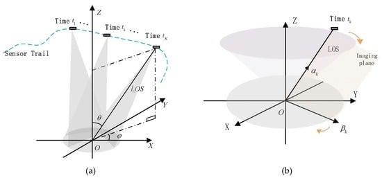
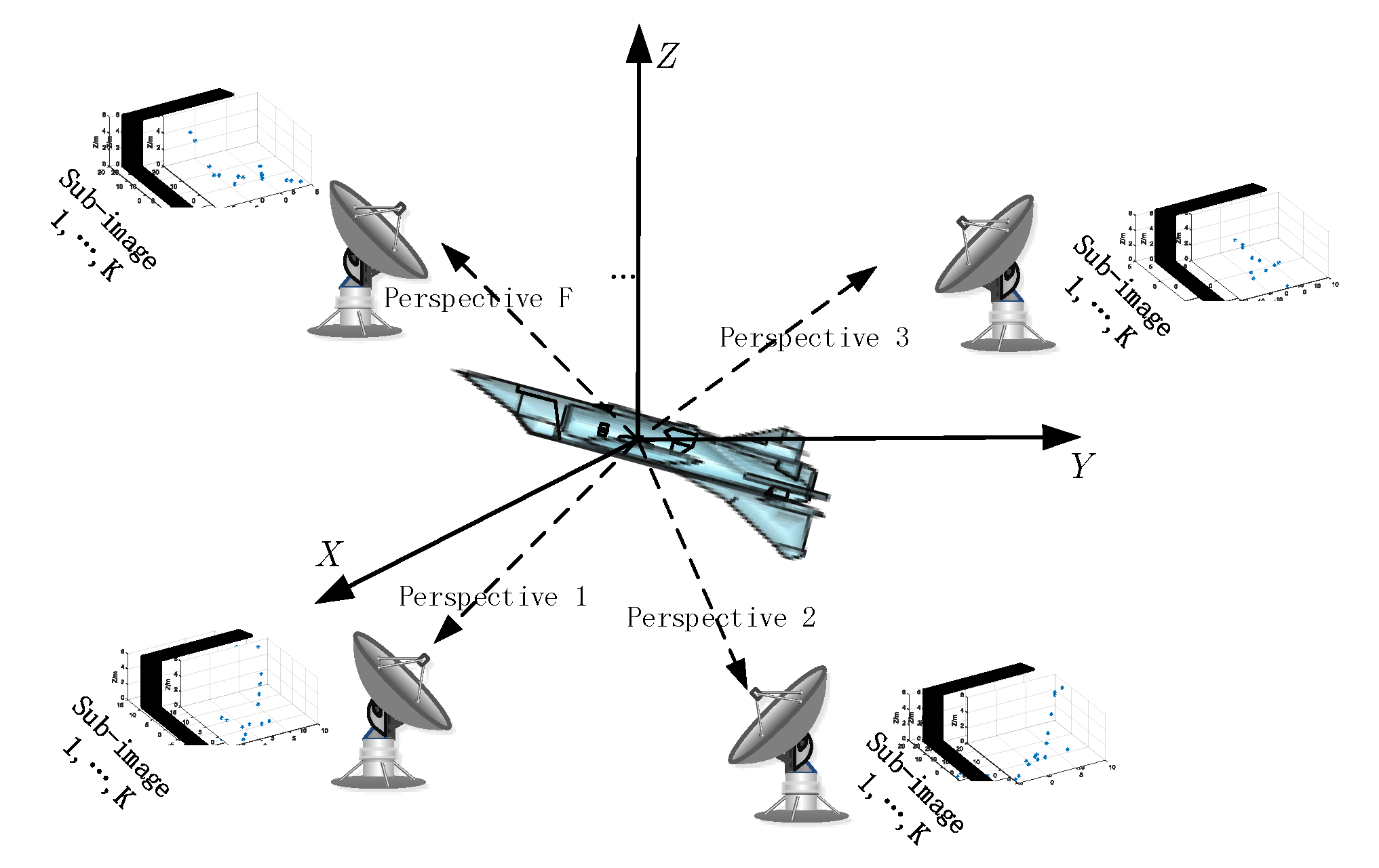
For wide-angle target echoes, it is necessary to divide the raw data into overlapped sub-apertures to perform translational motion compensation and dominant scatter centers extraction. Assume that the total number of sub-apertures is . The motion that comes from either a target or a radar, after translational motion compensation, can be molded as the radar rotation around a stationary target, which is shown in Figure 1a. In the kth sub-image, the unit projection vectors and in the imaging plane are shown in Figure 1b, where and represent range and azimuth dimensions in the kth imaging plane, respectively.
The established coordinate system is centered at the target. Assume that the target contains scattering centers, and the position of the th scatterer is denoted as , , where represents the transpose. For a maneuvering motion, the relative rotation velocity of LOS varies with sub-aperture, denoted as , . The rotation direction is the same as the axis, denoted as . During the observation time, the initial azimuthal angle of the LOS is , the elevation angle of the LOS remains constant, denoted as , which can be estimated by searching and will be described later.
In the kth sub-image, the unit projection vector of LOS in range dimension is formulated as
where denotes the middle time in the kth sub-image. The unit projection vector in azimuth dimension is represented as,
where denotes cross product. In general, the 2D radar image is the projection of the 3D target onto the imaging plane. Suppose that the scattering center at the kth sub-image imaging plane is represented as , where and are the projection locations in range and azimuth directions, respectively. Then the can be computed as,
The projection results at all times can be represented in a matrix form as,
where denotes the trajectory matrix of the scattering center locations in 2D image plane. denotes the element at the kth row and the column of given by,
, and , is modeled by Gaussian noise, denotes the projection matrix represented as,
where denotes the kth row of . Equation (4) reveals the projection process from 3D space to 2D space.
3. Theory and Method
3.1. Traditional 3D Geometry Reconstruction Based on Factorization Method
In order to illustrate the problem, We give a brief description about the process of 3D reconstruction based on matrix factorization [25,26].
First, the singular value decomposition (SVD) of is
where , and if . From (4), it can be seen that the rank of the trajectory matrix is 3 under the noiseless scenario. Although the rank of may not be strictly equal to 3 when there is noise, is a diagonal matrix with three dominant singular values. Let collect the elements in the first three columns and three rows of , denotes the first three columns of , denotes the first three columns of . Then the projection matrix and scatterer 3D position can be estimated as
where , and represent the estimates of and , respectively, where and , is a nonsingular matrix used to adjust to conform to the properties of projection matrix. Since and appear in pairs, they are called projection vector pairs in this paper. They satisfy the following constraints
Finally, matrix and projection vector pairs can be obtained by solving the equations in (9). Therefore, the target 3D geometry reconstruction, , can be obtained by (8). The detailed description of 3D geometry reconstruction based on factorization method can be found in [25,26].
In a given coordinate system, the scatter positions, i.e., , is defined as the attitude of the target in this paper, which can be used to estimate the motion of the target. Although the target attitude is estimated in (8), there are too many solutions for due to the insufficiency of the constraints in (9). Therefore, the estimate of the target attitude is still undetermined. More details are given in the following.
3.2. Analysis and Estimation of 3D Reconstruction Attitude
The constraints in (9) can only ensure that the projection vector pairs and are orthogonal unit vectors. However, the number of the orthogonal unit vector pairs is infinite. In particular, there is an arbitrary 3D rotation matrix which is called an ambiguity rotation matrix between these pairs, i.e., for any 3 by 3 unitary matrix with , and also satisfy (8) for the estimated attitude .
Ignoring the noise, (4) can be rewritten as
where is the kth row of . Therefore, the existence of the ambiguity rotation matrix can arbitrarily change the target attitude retrieved by the traditional 3D reconstruction. Due to the ambiguity rotation matrix , the projection matrix and the corresponding target attitude can be represented as
where and are, respectively, the projection matrix and the target attitude after changed by an arbitrary 3D rotation matrix . Under the conditions in (9), (10) holds, the arbitrary 3D rotation matrix at each sub-image is different, and the attitude obtained at each sub-image is also different. The projection matrix and target attitude at the sub-image can be formulated as
In order to analyze and solve the target attitude estimation problem, the following content is divided into three parts. They are the characteristics analysis of the arbitrary 3D rotation matrix , the influence of on the projection vector pairs and the influence on the estimated target attitude.
Under the influence of the ambiguity rotation matrix , the attitude of the target is unknown. Considering the motion of the LOS, by transforming projection vectors and into projection directions and , respectively, the target attitude can be changed into the same coordinate system.
The analysis above is based on the assumption that the LOS is in rotation motion and the target is stationary. However, it is more meaningful to observe the motion and attitude changes of the target rather than the radar. Therefore, the following analysis is based on the assumption that the target rotates around axis and the LOS is fixed.
Assume that the LOS is fixed in plane and has an angle with the axis. is unknown, but it will be estimated later. Then the corresponding unit projection vectors in range and azimuth directions can be expressed by and , respectively, as follows
The matrix satisfies the following formula
where , and denote the first to the third column vector of . To get the and that are consistent with and , respectively, several additional constraints are added to the projection vector pairs in two steps.
In the first step, the constraint in the third dimension can be expressed by
where is the intersection angle between vector and . Equation (15) means that and are orthogonal to each other, and the intersection angle is equivalent to because and are unit vectors.
In the second dimension, the constraint can be written as
Equation (16) means that and are orthogonal to each other, and is equivalent to .
On the other hand, the ambiguity rotation matrix must conform to the traits of the rotation matrix. Considering (15) and (16), the additional constraints on projection vector pairs are
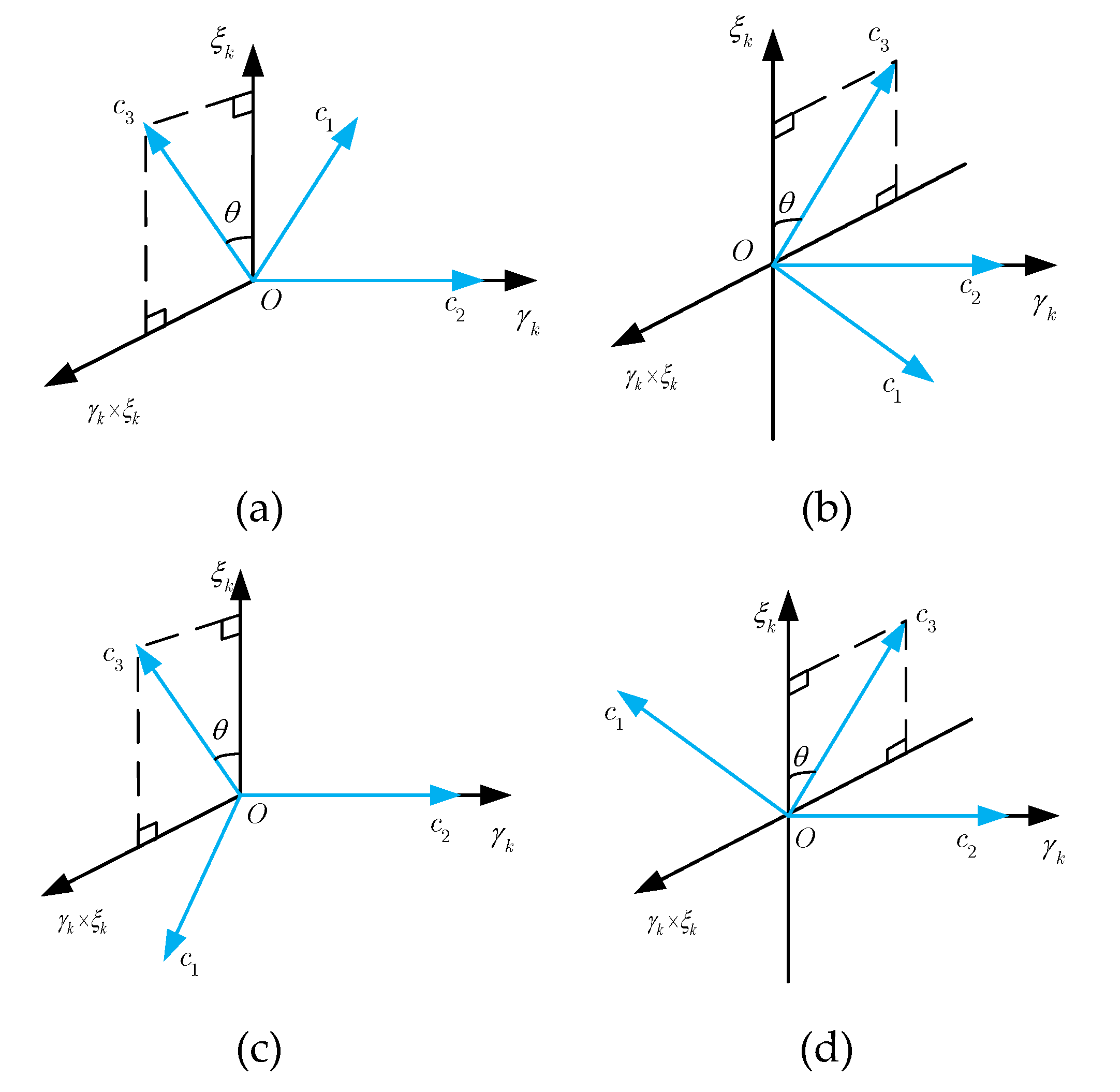
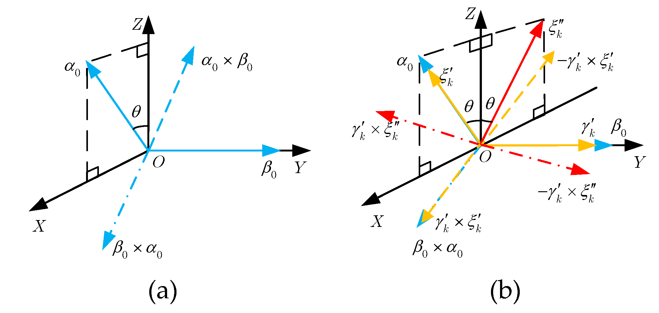
The constraints in (17) can be divided into two parts, and . By solving , two possible results of can be obtained. Since cannot distinguish and , the vector distributes on both sides of with an angle , as shown in Figure 2a,b. The constraint in can ensure that is a unit vector which is perpendicular to the plane of . In addition, the direction of can be upward or downward. Therefore, the constraint in has another possible expression:
Combining with the two possible solutions of , there are four possible solutions, denoted by , for , which stands for four different results of . The relationship between the constraints and the corresponding vectors is illustrated in Figure 2. The illustration of Equation (17) corresponds to Figure 2a,b, and that of Equation (18) corresponds to Figure 2c,d.
Based on the above analysis, can be written as
where denotes the column vector of , , , , denotes the rotation around the vector . The relationship of these four cases of is as follows: from (19), one can see that is the same in all four cases, that is . in (19.1) and (19.3) has opposite directions. This is also true for (19.2) and (19.4). Comparing (19.1) and (19.4), there exists a rotation relationship for with rotation angle around . is obtained by the cross product of and . Because the difference of , in (19.1) and (19.4) is also different from each other.
Due to the four cases of , the estimated projection matrix and the estimated target attitude will have four corresponding results. These results are related to each other. Suppose that the estimated projection vectors in range and azimuth directions are denoted by and , respectively. According to (14), we have
The placement of projection vectors in range and azimuth directions and in the coordinate system is shown in Figure 3a.
Combining (17.2), (19) and (20.1), one can see that the estimated projection vector in range direction has two values, expressed as and , respectively. Their angles with axis in the two sides of axis are , so one of them must be the same as . Suppose that is the same as , then there are four cases in the orthogonal coordinate system composed of , and ,, as shown in Figure 3b. In Figure 3b, only one case of makes the estimation projection vectors the same as that of (13), which is denoted as . The result of on attitude is the attitude which only rotates around axis.
On the other side, the estimated attitude from (12.2) can be rewritten as
where , , , , and denote the first to the third row vectors of . In this paper, is also called the third dimension of the target. Assume that the transformation result of on is taken as reference. Then, the effect of on is as follows:
makes the first dimensional vector of reverse, the third dimension is consistent with that of . makes rotate around . The effect of on is as follows: first, rotates around , then the first dimensional vector of the rotated result is reversed. The third dimension of the target attitude is the same as that of the attitude obtained from .
Four possible results through the function of can be obtained at each time and there exists a certain relationship among them. In order to find the among these four cases, the following process is proposed.
After solving the equations in (17), the target attitude can be represented as
where denotes the attitude after rotation through an ambiguity rotation matrix at .
As analyzed before, the target attitude is rotating around axis and varies with time . Suppose that the ambiguity rotation matrix at the sub-image is to be estimated. For the and the sub-image, the third dimension of the target coordinate does not change. In addition, the elevation angle of the LOS is usually unknown. If we give an incorrect angle , then the third dimension of the estimated target attitude may vary with time as well. Then, the elevation angle is estimated by searching a range of angles so that a more accurate can be obtained which makes the third dimension difference smaller. Therefore, the estimation of can be computed by
where denotes the Frobenius norm, denotes the third row vector of . Then the target attitude at the kth sub-image can be given by (22) with the rotation matrix in (23):
Although is different at different sub-images, the attitude of several sub-images can be obtained by one perspective and it is not necessary to calculate the of each sub-image.
3.3. Joint Multi-Perspective 3D Reconstruction
Generally speaking, the number of target dominate scatterers varies with different perspectives due to anisotropy and occlusion of scattering centers. This makes it possible to improve the representation of target features, increase target information and improve target visibility by performing multi-perspective 3D reconstruction. In this paper, the 3D imaging results are illustrated in the form of point clouds. Suppose that the total number of the perspectives is and these perspectives are from radars. The azimuth and the elevation angle of these radar LOSs are different, as shown in Figure 4. In Figure 4, there is sub-images in each perspective, and the number of scatterers and target attitudes obtained from each radar 3D imaging vary with the angle of view. Although these radar LOSs are different, the attitudes obtained from Section 3.2 are in the coordinate system with its own rotation axis as axis. Therefore, the target coordinates from these perspectives can coincide with each other by only one-dimensional rotation, that is, rotation around axis. The multi-perspective scattering fusion includes two parts. One is to find the target attitude relationship among different perspectives and the other is to fuse the point cloud based on the positions in different perspectives.
3.3.1. Target Attitude Relationship
In Section 3.2, it reveals that the target attitude relationship among different perspectives is a rotation around the axis. Therefore, a 3D point cloud matching among different perspectives is needed before information fusion. Assume that there is a sequence of 3D images in perspectives with different numbers of feature points. The number of the scatterers in the fth perspective is denoted as determined by the dominant scatter center extraction methods [28,29,30]. Then the scatterer coordinates are described as
Let and denote target attitudes in the perspective and the perspective, respectively. In order to get the target attitudes and matched to each other, the target attitude needs to rotate an angle around the axis, described as
where denotes the rotation around the axis:
Then under the rotation angle , the average distance of scattering points from perspective to perspective can be described as
where denotes the minimum Mahalanobis distance among the ranges from the scatterer in the perspective to all the scatteres in the perspective, described as
Finally, the distance between the and the perspectives can be obtained by solving
The closer the angle is to the true value, the smaller the distance is. The process of searching for is summarized as follows:
Step 1: Initialize the rotation angle range , is a constant value that does not change in each iteration, and are pre-set thresholds set by experience, , .
Step 2: Sample the rotation angle in the range with interval , .
Step 3: The distance is computed and denoted as . Let .
Step 4: If and , or , then stop the iteration and go to Step 6.
Step 5: If , let and ; If , let and ; If and , let and . Then , , and go to Step 2.
Step 6: The estimated rotation angle is .
3.3.2. Point Cloud Fusion
When all perspective images are transformed into the same coordinate system by using (27), the scatterers of different images will overlap, which will cause information redundancy. Then the position of the fused scattering point is expressed as
Since several scatterers can be observed from each perspective, the number of scatterers obtained by multi-perspective 3D reconstruction will increase with the increase of the number of perspectives. The target integrity will be further improved. The integrity of multi-perspective 3D reconstruction is defined as the ratio of the number of scatterers detected to the total number of the target scatterers.
3.4. Algorithm Summation
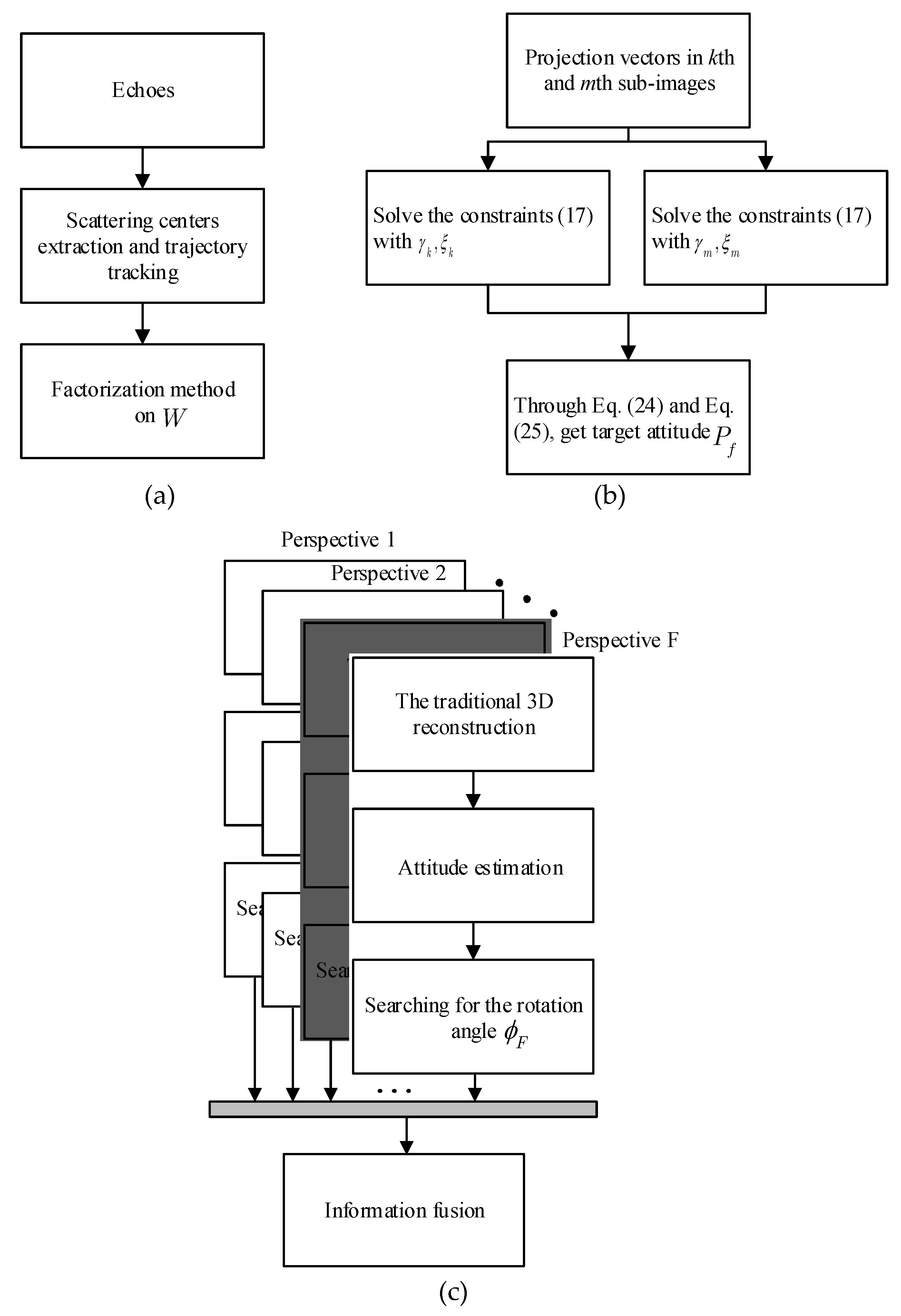
After performing scattering center extraction and trajectory tracking, the trajectory matrix can be obtained. Then the factorization method is applied to the trajectory matrix. The target structure with unknown attitude is obtained from the traditional 3D reconstruction shown in Figure 5a. The matrix factorization may have a unitary ambiguity 3D rotation matrix which in turn affects the target attitude of the traditional 3D reconstruction. Therefore, a further processing is adopted to estimate the unitary ambiguity 3D rotation matrix to obtain the desired target attitude, as shown in Figure 5b. Finally, the multi-perspective 3D reconstruction can be obtained by multiple perspective information fusion. Because multi-perspective 3D reconstruction is performed on the 3D reconstruction results generated by each perspective, there is no requirement on the location of radars and the time of observation. Compared with InISAR, the multi-perspective 3D reconstruction is more flexible and less expensive than InISAR in terms of equipment requirements, although multiple radars may be needed. The proposed method is illustrated by flowchart in Figure 5c.
4. Simulations
In this section, several simulation results based on the point-scatterer model are presented to verify the effectiveness and noise insensitive of the proposed method. In the first experiment, a simple shape object is used to verify the accuracy of the proposed single perspective target attitude estimation. Meanwhile, the effectiveness of the proposed method is evaluated by comparing with the traditional 3D reconstruction. For a complex target, due to occlusion and scattering characteristics, the target obtained from a single perspective is relatively simple. In the second experiment, on the basis of the attitude estimation, the 3D reconstruction results from multiple perspectives are converted to one coordinate system and fused together. Then a more complex target can be obtained.
4.1. Single Perspective Attitude Estimation
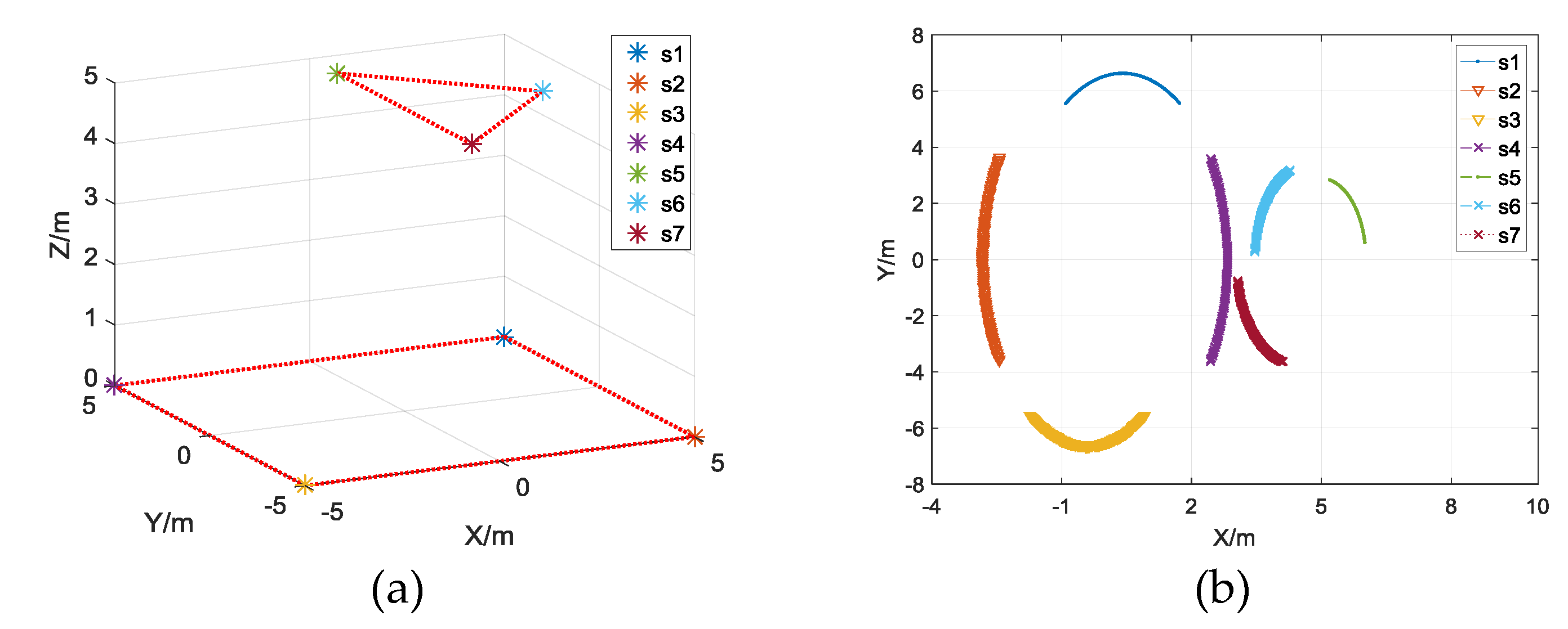
An asymmetric target shown in Figure 6a is used to verify the accuracy of target attitude estimation of the proposed method, where ‘s n’ denotes the nth scatterer. The simulated target consists of seven scatterers and rotates around the axis at 0.069 rad/s speed.
The simulated radar operates in the X-band with transmitted signal bandwidth of 2 GHz and the range resolution is 0.075m. The azimuth and the elevation angle of the radar LOS are 0 and rad, respectively. The total observation time is 16.5s and the corresponding rotational angle is 66 degrees which is divided into 100 overlapped sub-images. By extraction and tracking of these scatterers, the trajectory matrix is formed, as shown in Figure 6b.
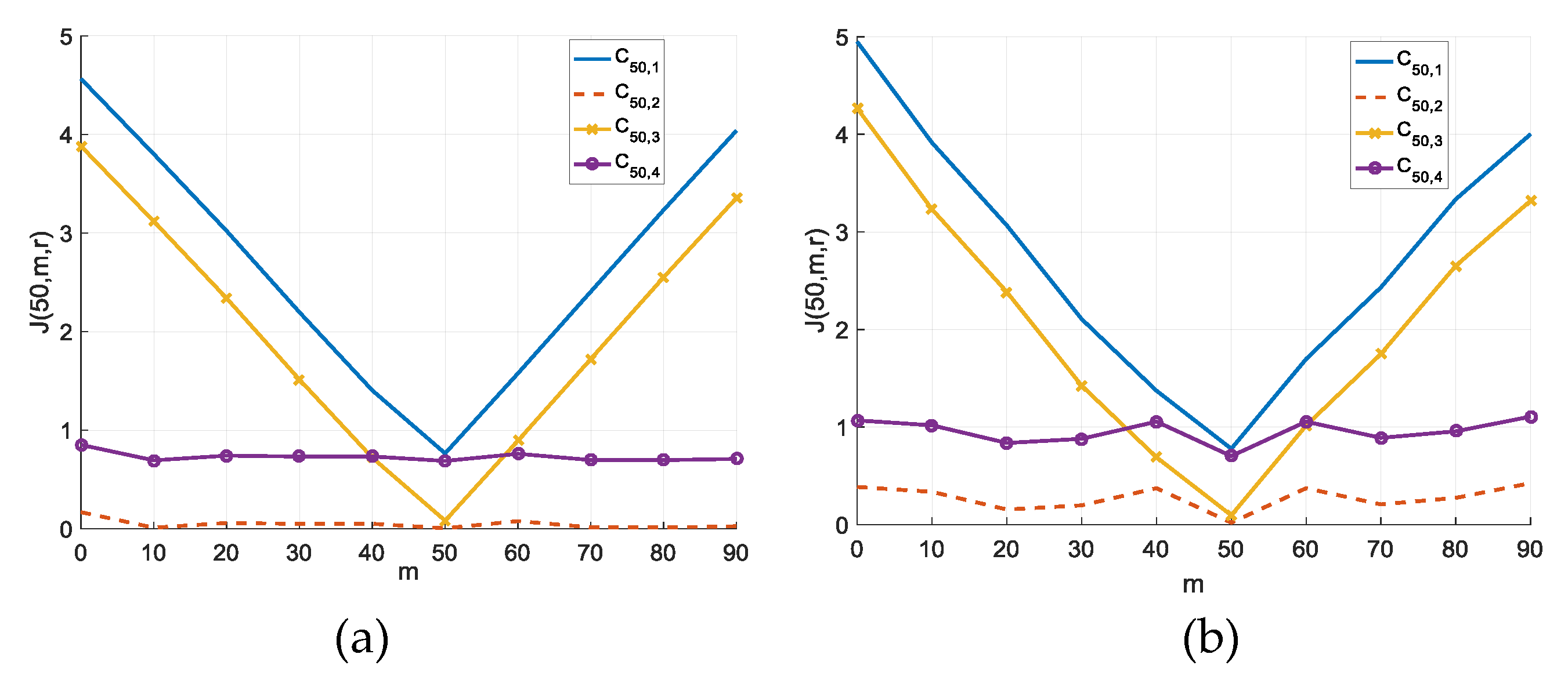
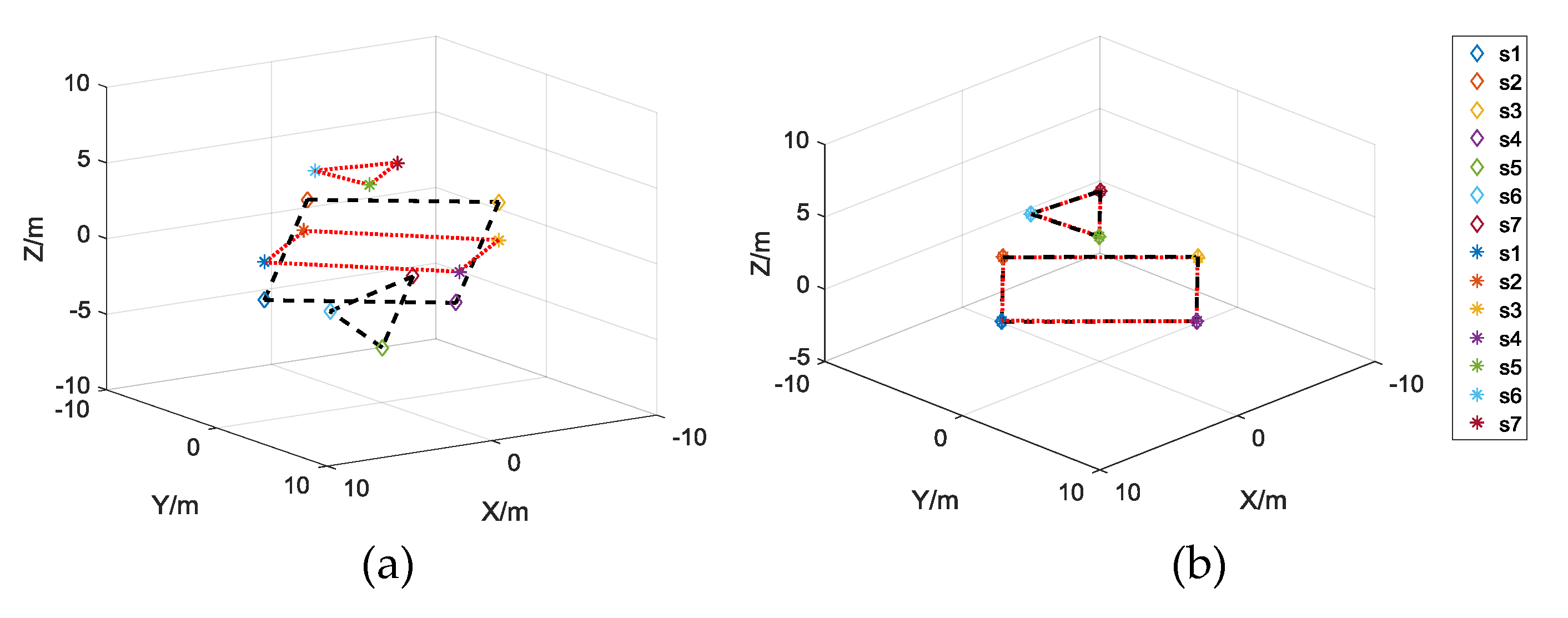
The extraction and tracking errors of scatterers will influence the performance of the 3D reconstruction. To analyze the effect of trajectory error on the attitude estimation, Gaussian noises with the standard deviation of 0.5, and 5 times of the range resolution are added to the scatterer trajectory matrix to simulate scatterers extraction and tracking errors, respectively. The follow experiments take the results of the 50th sub-image as an example. After attitude estimation, the result of generated from the unitary ambiguity 3D rotation matrix is shown in Figure 7, where horizontal coordinate is the index of sub-image. Figure 7a,b are obtained under the condition of Gaussian noises with the standard deviation of 0.5 and 5 times of the range resolution, respectively. Since taking the results of the 50th sub-image as an example, can achieve its smallest value when m is 50. In Figure 7, is the smallest in all the sub-images. Therefore, it is sufficient to calculate (24) with a sub-image when the difference between m and 50 is large. Moreover, this shows that is the required unitary ambiguity 3D rotation matrix. The results of 3D reconstruction are shown in Figure 8, where different colors denote different scatterers, ‘s n’ denotes the nth scatterer. The stars denote the real location at the corresponding time and the diamonds denote scatterer locations of the 3D reconstruction. In Figure 8a, the attitude of the traditional 3D reconstruction is varied arbitrarily because of the existence of the unitary ambiguity 3D rotation matrix. After attitude estimation, the reconstruction attitude is consistent with the real attitude as shown in Figure 8b.
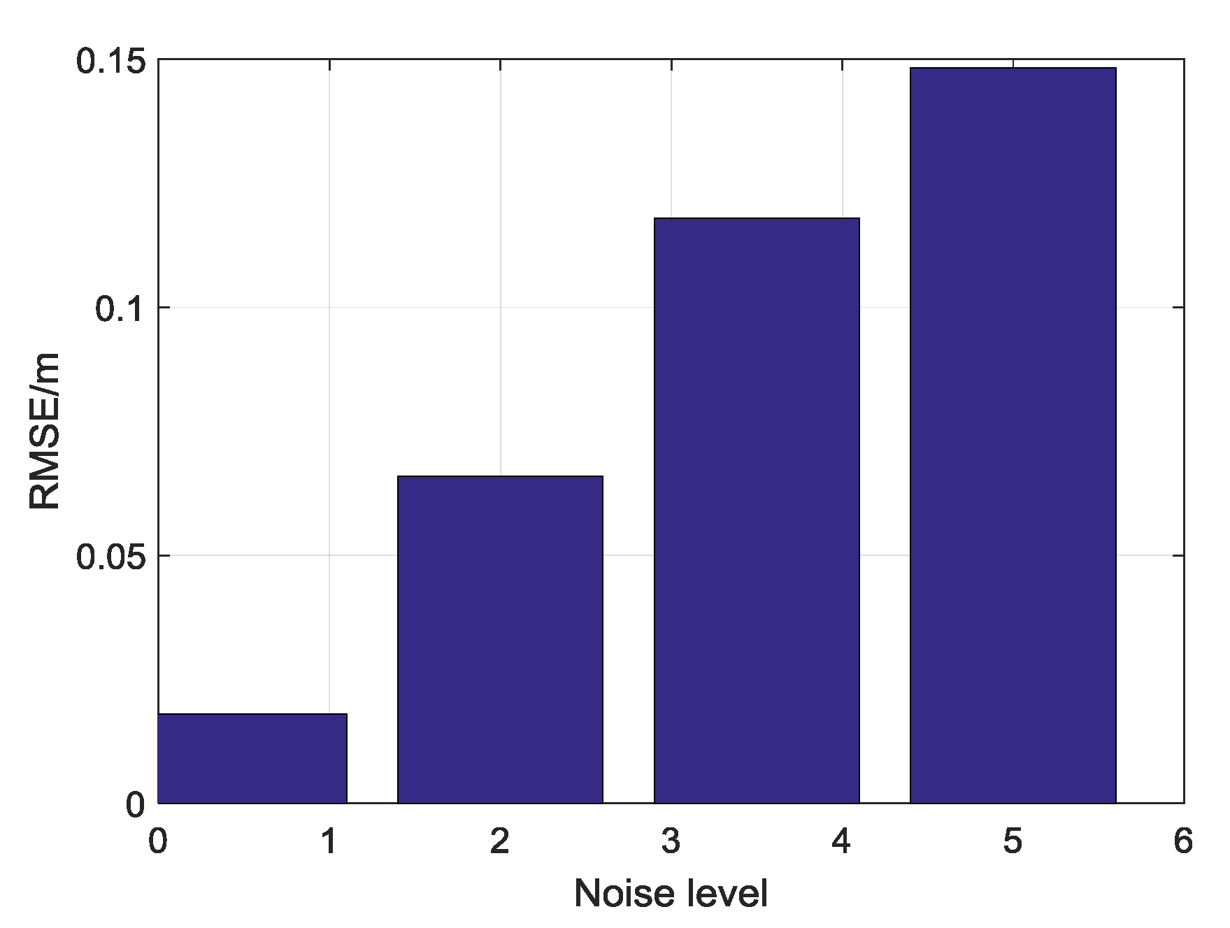
To evaluate the performance of the proposed method, the root mean square error (RMSE) of 3D reconstruction is employed, which is defined as
where is the target 3D reconstruction result, is the true target 3D geometry, is the number of target scatterers. As discussed above, the inaccurate extraction and tracking errors of the scatterers will degrade the performance of the proposed method. To obtain the RMSE of 3D reconstruction, 500 Monte-Carlo simulations are performed for each noise level ranging from 0.5 to 5 times of the range resolution. The experimental results are shown in Figure 9, which depicts the RMSE of the attitude estimation. Figure 9 shows that the accuracy of the proposed method decreases with the increase of noise level.
4.2. Multi-Perspective 3D Imaging Results
Using the target attitude estimation based on single perspective 3D reconstruction, multi-perspective 3D reconstruction can be accomplished. The 3D geometry of the simulated scatterer model is presented in Figure 10, which consists of 165 scatterers and rotates around the axis at 0.069 rad/s speed. The radar parameters are set to be the same as the first experiment. Generally speaking, the number and locations of scattering centers of the same target are different in different perspectives. In this experiment, three perspectives are chosen. In each perspective, it randomly chooses different number of scatterers of the target as the observable scatterers. In addition, the elevation and azimuth angles of the LOS from different perspectives are also different from each other.
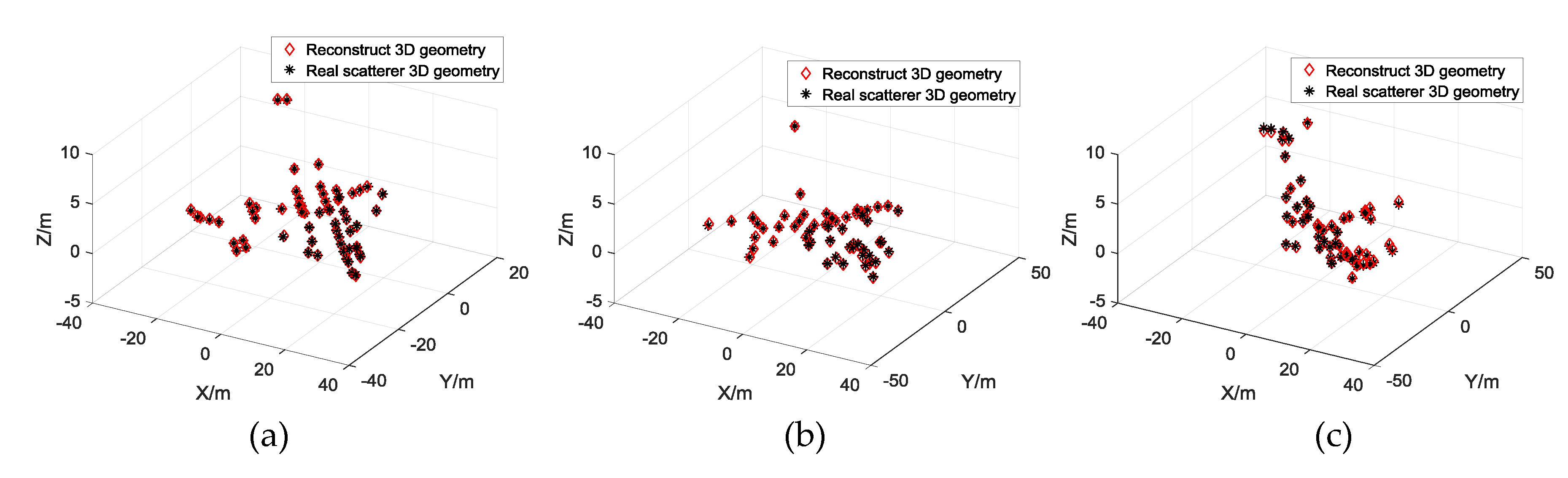
For the first perspective, the azimuth and the elevation angle of the radar LOS are 0 and 30 degrees, respectively. In this perspective, only 51 scatterers can be observed. These scatterers are mainly distributed in the main body and the left side of the airplane. For the second perspective, the azimuth and the elevation angle of the radar LOS are 30 and 25 degrees, respectively. In this perspective, only 58 scatterers can be observed. These scatterers are mainly distributed in the main body and the right side of the airplane. For the third perspective, the azimuth and the elevation angle of the radar LOS are 45 and 20 degrees, respectively. In this perspective, only 54 scatterers can be observed. These scatterers are mainly distributed in the main body of the airplane. Figure 11 shows the variation of the RMSE of 3D reconstruction with respect to elevation angle of the radar LOS. In Figure 11a,b, the estimation deviations of these two elevation angles are 0. Figure 11c shows that the estimation deviation of the third perspective elevation angle is less than 0.25 degrees. When the elevation angle equals to the true value, the RMSE of 3D reconstruction achieves the smallest value. Figure 12 shows the variation of the estimated attitudes with respect to the different perspectives. In Figure 12, the stars denote the real target attitude at the corresponding time and the diamonds denote the 3D reconstruction attitude. Figure 13 shows the variation of with the sub-images. Figure 13a is obtained when the rotational velocity is 10 degrees per second and noise level is 5 times range resolution. In order to clearly observe the variation of , Figure 13b magnifies the change near the 50th sub-image. As can be seen from Figure 13a,b, is the required unitary ambiguity 3D rotation matrix. Finally, by rotating different sub-perspective 3D images based on Section 3.3, these 3D images are placed in the same coordinate system. After 3D point cloud information fusion, multi-perspective 3D results can be obtained.
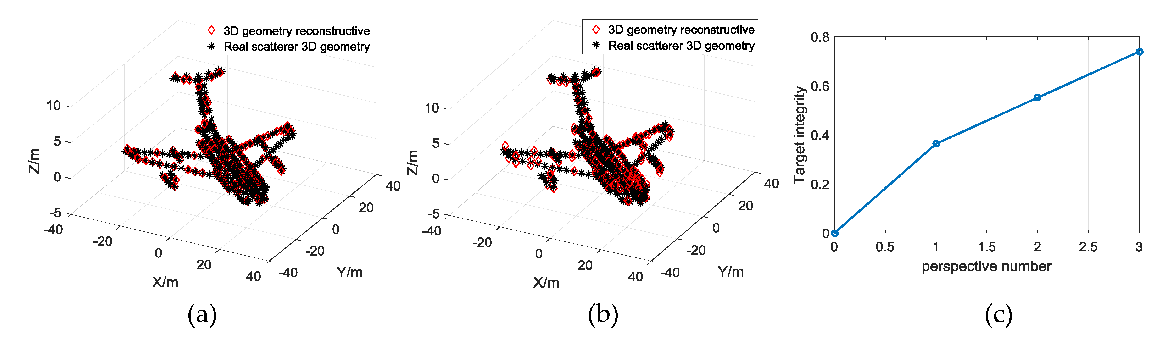
In order to evaluate the performance of the proposed method, 500 Monte-Carlo simulations are carried out to evaluate the influence of rotational velocity and noise level on the proposed method. The three perspectives, same as those in Figure 11, are used. The noise level is increased from 0.5 to 5 times of the range resolution in increments of 1.5. The rotational speed is increased from 2 to 10 degrees per second in increments of 1. In these simulations, the total rotation is 180 degrees and the total number of the sub-images is 100. Suppose that the required estimated attitude is from the 50th sub-image. The experimental results are presented in Figure 14 and Figure 15. The corresponding attitudes obtained from the multi-perspective 3D images are shown in Figure 14. Apparently, the accuracy of attitude estimation in Figure 14b is worse than that in Figure 14a. Figure 14c is obtained by performing 500 Monte-Carlo trails. It shows that the integrity of multi-perspective 3D reconstruction increases with the increase of the number of utilized perspectives, that is, the visibility is improved.
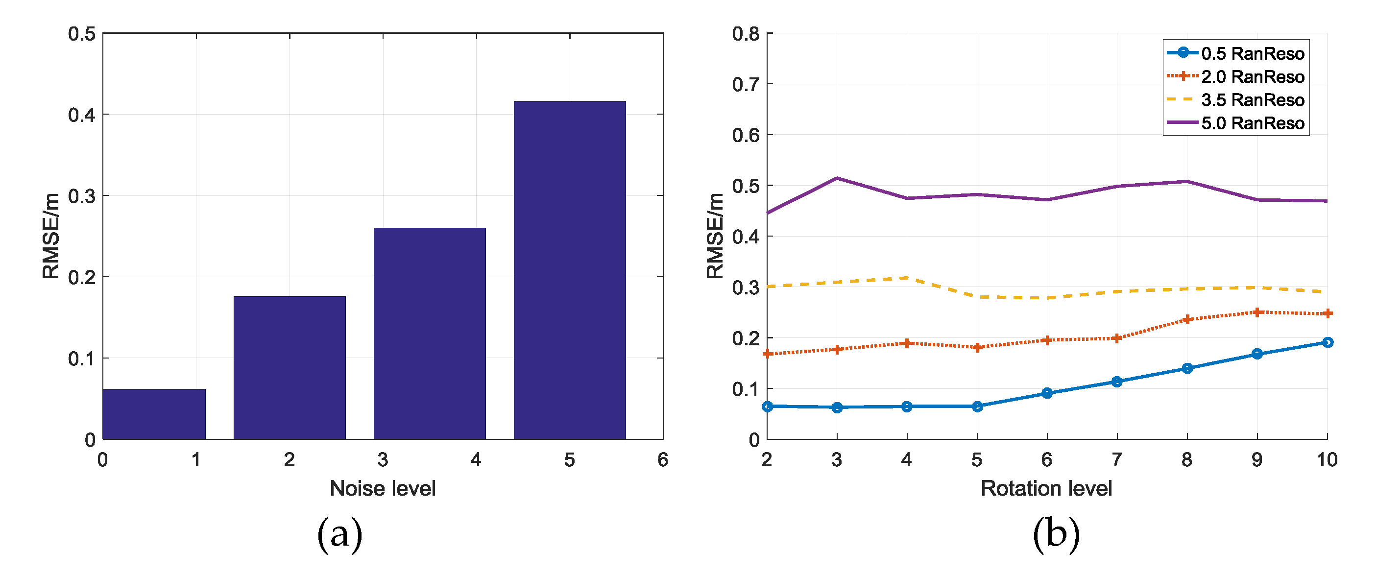
After 500 Monte-Carlo simulations, Figure 15 shows the variation of RMSE of multi-perspective 3D reconstruction with different noise level and rotational velocity. Since the accuracy of single perspective 3D reconstruction is mainly affected by the scatterer trajectory accuracy, the RMSE of the single perspective 3D reconstruction is increased as the noise level increases in Figure 15a. Figure 15b shows the variation of RMSE of multi-perspective 3D reconstruction with the rotational velocity level per noise level. When the noise level is relative low, such as 0.5 and 2.0 times of the range resolution, the RMSE of multi-perspective 3D reconstruction tends to become slightly larger as the rotational velocity increases. When the noise level is larger than 5 times of the range resolution, the effect of the rotational velocity on the performance of the multi-perspective 3D reconstruction method is not dominated. Meanwhile, for the rotational velocity is fixed, the RMSE of the multi-perspective 3D reconstruction becomes larger as the noise level increases, which indicates that the noise level has a greater effect on the accuracy of multi-perspective 3D reconstruction.
5. Conclusions
In order to deal with the limitation of 2D imaging about a 3D target, we need to carry out 3D imaging by multi-perspective 3D reconstruction. However, the target attitude obtained by the traditional 3D imaging method is unknown. Moreover, single perspective 3D reconstruction cannot provide the complete information of a target, since several scatterers may be missed in a single perspective. To solve the problem, this paper proposes a new method for multi-perspective 3D imaging with single perspective instantaneous target attitude estimation. The target attitude of single perspective 3D reconstruction is estimated first. Then, the target attitudes obtained from different perspectives are converted into the same coordinate. Finally, the redundant information is merged into single-layer information and the final 3D imaging result can be obtained. The effectiveness and noise insensitive of the proposed method is verified by several numerical examples. Compared with the single perspective traditional 3D reconstruction, the multi-perspective 3D imaging increases the target information and improves the visibility.
Author Contributions
Formal analysis, D.X., M.X., X.-G.X., G.-C.S., J.F. and T.S.; Writing—original draft, D.X.; Writing—review & editing, D.X. and X.-G.X.
Funding
This research was funded by the Foundation for Innovative Research Groups of the National Natural Science Foundation of China under Grant 61621005 and the National Science Found for Distinguished Young Scholars under Grant 61825105.
Acknowledgments
The authors would like to acknowledge the anonymous reviewers and Yongjun Liu for their useful comments and suggestions, which were great help in improving this paper. Meanwhile, this work is partially supported by the Fund for Foreign Scholars in University Research and Teaching Programs (the 111Project) (No. B18039).
Conflicts of Interest
The authors declare no conflict of interest.
References
- Chen, C.-C.; Andrews, H.C. Target-motion-induced radar imaging. IEEE Trans. Aerosp. Electron. Syst. 1980, 16, 2–14. [Google Scholar] [CrossRef]
- Zhang, Q.; Yeo, T.S.; Du, G. ISAR imaging in strong ground clutter using a new stepped-frequency signal format. IEEE Trans. Geosci. Remote Sens. 2003, 41, 948–952. [Google Scholar] [CrossRef]
- Wang, Q.; Xing, M.; Lu, G.; Bao, Z. Single range matching filtering for space debris radar imaging. IEEE Geosci. Remote Sens. Lett. 2007, 4, 576–580. [Google Scholar] [CrossRef]
- Lv, X.; Xing, M.; Wan, C.; Zhang, S. ISAR imaging of maneuvering targets based on the range centroid Doppler technique. IEEE Trans. Image Process. 2010, 19, 141–153. [Google Scholar] [PubMed]
- Wang, D.; Ma, X.; Chen, A.; Su, Y. High-resolution imaging using a wideband MIMO radar system with two distributed arrays. IEEE Trans. Image Process. 2010, 19, 1280–1289. [Google Scholar] [CrossRef]
- Chen, J.; Sun, G.; Xing, M.; Liang, B.; Gao, Y. Focusing improvement of curved trajectory spaceborne SAR based on optimal LRWC preprocessing and 2-D singular value decomposition. IEEE Trans. Geosci. Remote Sens. 2019. [Google Scholar] [CrossRef]
- Li, J.; Ling, H. 3D ISAR image reconstruction of a target with motion data using adaptive feature extraction. J. Electromagn. Waves Appl. 2001, 15, 1571–1587. [Google Scholar] [CrossRef]
- Mayhan, J.T.; Burrows, M.L.; Cuomo, K.M.; Piou, J.E. High resolution 3D ‘Snapshot’ ISAR imaging and feature extraction. IEEE Trans. Aerosp. Electron. Syst. 2001, 37, 630–642. [Google Scholar] [CrossRef]
- Stuff, M.A.; Sanchez, P.; Biancalana, M. Extraction of three dimensional motion and geometric invariants from range dependent signals. Multidimen. Syst. Signal Process. 2003, 14, 161–181. [Google Scholar] [CrossRef]
- Given, J.A.; Schmidt, W.R. Generalized ISAR—Part II: Interferometric techniques for three-dimensional location of scatterers. IEEE Trans. Image Process. 2005, 14, 1792–1797. [Google Scholar] [CrossRef] [PubMed]
- Wu, Z.; Zhang, L.; Liu, H. Generalized Three-dimensional imaging algorithms for synthetic aperture radar with metamaterial apertures-based antenna. IEEE Access 2019, 7, 1–12. [Google Scholar] [CrossRef]
- Zhou, J.; Shi, Z.; Fu, Q. Three-dimensional scattering center extraction based on wide aperture data at a single elevation. IEEE Trans. Geosci. Remote Sens. 2015, 53, 1638–1655. [Google Scholar] [CrossRef]
- Wang, G.; Xia, X.-G.; Chen, V. Three-dimensional ISAR imaging of maneuvering targets using three receivers. IEEE Trans. Image Process. 2001, 10, 436–447. [Google Scholar] [CrossRef]
- Xu, X.; Narayanan, R.M. Three-dimensional interferometric ISAR imaging for target scattering diagnosis and modeling. IEEE Trans. Image Process. 2001, 10, 1094–1102. [Google Scholar] [PubMed]
- Ma, C.; Yeo, T.S.; Zhang, Q.; Tan, H.; Wang, J. Three-dimensional ISAR imaging based on antenna array. IEEE Trans. Geosci. Remote Sens. 2008, 46, 504–515. [Google Scholar] [CrossRef]
- Duan, G.; Wang, W.; Ma, X.; Su, Y. Three-dimensional imaging via wideband MIMO radar system. IEEE Geosci. Remote Sens. Lett. 2010, 7, 445–449. [Google Scholar] [CrossRef]
- Ma, C.; Yeo, T.S.; Tan, C.; Tan, H. Sparse array 3-D ISAR imaging based on maximum likelihood estimation and clean technique. IEEE Trans. Image Process. 2010, 19, 2127–2142. [Google Scholar] [PubMed]
- Suwa, K.; Wakayama, T.; Iwamoto, M. Three-dimensional target geometry and target motion estimation method using multistatic ISAR movies and its performance. IEEE Geosci. Remote Sens. 2011, 6, 2361–2373. [Google Scholar] [CrossRef]
- Martorella, M.; Salvetti, F.; Stagliano, D. 3D target reconstruction by means of 2D-ISAR imaging and interferometry. In Proceedings of the 2013 IEEE Radar Conf. (RADAR), Ottawa, ON, Canada, 29 April–3 May 2013; pp. 1–6. [Google Scholar]
- Liu, Y.; Song, M.; Wu, K.; Wang, R.; Deng, Y. High-quality 3-D InISAR imaging of maneuvering target based on a combined processing approach. IEEE Geosci. Remote Sens. Lett. 2013, 10, 1036–1040. [Google Scholar]
- Xu, G.; Xing, M.; Xia, X.-G.; Zhang, L.; Chen, Q.; Bao, Z. 3D Geometry and motion estimations of maneuvering targets for interferometric ISAR with sparse aperture. IEEE Trans. Image Process. 2016, 25, 2005–2020. [Google Scholar] [CrossRef]
- Knaell, K.; Cardillo, G. Radar tomography for the generation of three-dimensional images. Proc. Inst. Elect. Eng.—Radar Sonar Navig. 1995, 142, 54–60. [Google Scholar] [CrossRef] [Green Version]
- Tomasi, C.; Kanade, T. Shape and motion from image streams under orthography: A factorization method. Int. J. Comput. Vis. 1992, 9, 137–154. [Google Scholar] [CrossRef]
- Morita, T.; Kanade, T. A sequential factorization method for recovering shape and motion from image streams. IEEE Trans. Pattern Anal. Mach. Intell. 1997, 19, 858–867. [Google Scholar] [CrossRef]
- McFadden, F.E. Three-dimensional reconstruction from ISAR sequences. Proc. SPIE 2002, 4744, 58–67. [Google Scholar]
- Liu, L.; Zhou, F.; Bai, X.; Tao, M. Joint cross-range scaling and 3D Geometry reconstruction of ISAR targets based on factorization method. IEEE Trans. Image Process. 2016, 25, 1740–1750. [Google Scholar] [CrossRef] [PubMed]
- Wang, F.; Xu, F.; Jin, Y. 3-D information of a space target retrieved from a sequence of high-resolution 2-D ISAR images. In Proceedings of the 2016 IEEE International Geoscience and Remote Sensing Symposium (IGARSS), Beijing, China, 10–15 July 2016. [Google Scholar]
- Wang, F.; Xu, F.; Jin, Y. Three-dimensional reconstruction from a multiview sequence of sparse ISAR imaging of a space target. IEEE Trans. Geosci. Remote Sens. 2018, 56, 611–620. [Google Scholar] [CrossRef]
- Paulraj, A.; Roy, R.; Kailath, T. Estimation of signal parameters via rotational invariance techniques-ESPRIT. IEEE Trans. Acoust. 1989, 37, 984–995. [Google Scholar]
- Wang, X.; Zhang, M.; Zhao, J. Super-resolution ISAR imaging via 2D unitary ESPRIT. Electron. Lett. 2015, 51, 519–521. [Google Scholar] [CrossRef]
- Wu, M.; Xing, M.; Zhang, L.; Duan, J.; Xu, G. Super-resolution imaging algorithm based on attributed scattering center model. In Proceedings of the 2014 IEEE China Summit & Ingernational Conference on Signal and Information Processing (ChinaSIP), Xi’an, China, 9–13 July 2014; pp. 271–275. [Google Scholar]
- Oh, S.; Russell, S.; Sastry, S. Markvo chain Monte Carlo data association for multi-target tracking. IEEE Trans. Autom. Control. 2009, 54, 481–497. [Google Scholar]
- Liu, L.; Zhou, F.; Bai, X. Method for scatterer trajectory association of sequential ISAR images based on Markvo chain Monte Carlo algorithm. IET Radar Sonar Navig. 2018, 12, 1535–1542. [Google Scholar] [CrossRef]
- Zhou, Y.; Zhang, L.; Xing, C.; Xie, P.; Cao, Y. Target three-dimensional reconstruction from the multi-view radar image sequence. IEEE Access. 2019, 7, 36722–36735. [Google Scholar] [CrossRef]
- Zhang, L.; Sheng, J.; Duan, J.; Xing, M. Translational motion compensation for ISAR imaging under low SNR by minimum entropy. EURASIP J. Adv. Signal Process. 2013. [Google Scholar] [CrossRef]
Figure 1.
Radar position and the projection vectors of the kth imaging plane. (a) The rotation relationship between the LOS and the target. (b) The two-dimensional projection vectors of the kth imaging plane.
Figure 1.
Radar position and the projection vectors of the kth imaging plane. (a) The rotation relationship between the LOS and the target. (b) The two-dimensional projection vectors of the kth imaging plane.

Figure 2.
Four different possible results of . (a) For , locates at the left side of . (b) For , locates at the right side of . (c) For , is perpendicular to the plane and downward. (d) For , is perpendicular to the plane and upward.
Figure 2.
Four different possible results of . (a) For , locates at the left side of . (b) For , locates at the right side of . (c) For , is perpendicular to the plane and downward. (d) For , is perpendicular to the plane and upward.

Figure 3.
Placement of projection vectors. (a) Placement of and . (b) Placement of four cases of the estimated projection vectors.
Figure 3.
Placement of projection vectors. (a) Placement of and . (b) Placement of four cases of the estimated projection vectors.

Figure 4.
The model of multiple perspectives.

Figure 5.
Algorithm of multi-perspective 3D reconstruction summary. (a) The traditional 3D reconstruction. (b) The procedure of attitude estimation for the fth perspective. (c) Multi-perspective 3D imaging.
Figure 5.
Algorithm of multi-perspective 3D reconstruction summary. (a) The traditional 3D reconstruction. (b) The procedure of attitude estimation for the fth perspective. (c) Multi-perspective 3D imaging.

Figure 6.
The model of the simulated target. (a) The point-scatterer model. (b) The scatterer trajectories.
Figure 6.
The model of the simulated target. (a) The point-scatterer model. (b) The scatterer trajectories.

Figure 7.
The effect of the unitary ambiguity 3D rotation matrix on the 50th sub-image. (a) The noise is 0.5 times of the range resolution. (b) The noise is 5 times of the range resolution.
Figure 7.
The effect of the unitary ambiguity 3D rotation matrix on the 50th sub-image. (a) The noise is 0.5 times of the range resolution. (b) The noise is 5 times of the range resolution.

Figure 8.
The attitudes from the 3D reconstruction result with the standard derivation of the noise is set to be half of the range resolution. (a) The traditional 3D reconstruction. (b) The proposed 3D reconstruction.
Figure 8.
The attitudes from the 3D reconstruction result with the standard derivation of the noise is set to be half of the range resolution. (a) The traditional 3D reconstruction. (b) The proposed 3D reconstruction.

Figure 9.
RMSE of 3D reconstruction proposed in this paper after 500 Monta-Carlo experiments.

Figure 10.
The model of experiment.

Figure 11.
The estimations of the elevation angle of the three perspectives. (a)~(c) Variation of the RMSE of 3D reconstruction with respect to the elevation angle of the radar LOS in different perspectives.
Figure 11.
The estimations of the elevation angle of the three perspectives. (a)~(c) Variation of the RMSE of 3D reconstruction with respect to the elevation angle of the radar LOS in different perspectives.

Figure 12.
Variation of estimated attitudes of 3D reconstruction from three different perspectives. (a)~(c) The attitudes obtained by the proposed method from different perspectives.
Figure 12.
Variation of estimated attitudes of 3D reconstruction from three different perspectives. (a)~(c) The attitudes obtained by the proposed method from different perspectives.

Figure 13.
Variation of with the respect to the sub-images. (a) when the rotational velocity is 10 degrees per second and noise level is 5 times range resolution. (b) Local enlargement result of .
Figure 13.
Variation of with the respect to the sub-images. (a) when the rotational velocity is 10 degrees per second and noise level is 5 times range resolution. (b) Local enlargement result of .

Figure 14.
The estimated attitudes of multi-perspective 3D reconstruction from different conditions. (a) The estimated attitudes of multi-perspective when the rotational velocity is 2 degrees per second and noise level is 0.5 times range resolution. (b) The estimated attitudes of multi-perspective when the rotational velocity is 10 degrees per second and noise level is 5 times range resolution. (c) The integrity of multi-perspective 3D reconstruction varies with the number of utilized perspectives.

Figure 15.
Variation of RMSE of multi-perspective 3D reconstruction with the noise level and rotation velocity level. (a) Variation of RMSE with respect to noise level when rotation velocity is 2 degrees per second. (b) Variation of RMSE with respect to rotation velocity level per noise level.
Figure 15.
Variation of RMSE of multi-perspective 3D reconstruction with the noise level and rotation velocity level. (a) Variation of RMSE with respect to noise level when rotation velocity is 2 degrees per second. (b) Variation of RMSE with respect to rotation velocity level per noise level.

© 2019 by the authors. Licensee MDPI, Basel, Switzerland. This article is an open access article distributed under the terms and conditions of the Creative Commons Attribution (CC BY) license (http://creativecommons.org/licenses/by/4.0/).
Share and Cite
MDPI and ACS Style
Xu, D.; Xing, M.; Xia, X.-G.; Sun, G.-C.; Fu, J.; Su, T. A Multi-Perspective 3D Reconstruction Method with Single Perspective Instantaneous Target Attitude Estimation. Remote Sens. 2019, 11, 1277. https://doi.org/10.3390/rs11111277
AMA Style
Xu D, Xing M, Xia X-G, Sun G-C, Fu J, Su T. A Multi-Perspective 3D Reconstruction Method with Single Perspective Instantaneous Target Attitude Estimation. Remote Sensing. 2019; 11(11):1277. https://doi.org/10.3390/rs11111277
Chicago/Turabian StyleXu, Dan, Mengdao Xing, Xiang-Gen Xia, Guang-Cai Sun, Jixiang Fu, and Tao Su. 2019. "A Multi-Perspective 3D Reconstruction Method with Single Perspective Instantaneous Target Attitude Estimation" Remote Sensing 11, no. 11: 1277. https://doi.org/10.3390/rs11111277
Note that from the first issue of 2016, this journal uses article numbers instead of page numbers. See further details here.