Mapping Annual Forest Change Due to Afforestation in Guangdong Province of China Using Active and Passive Remote Sensing Data


Abstract
:
1. Introduction
2. Materials and Methods
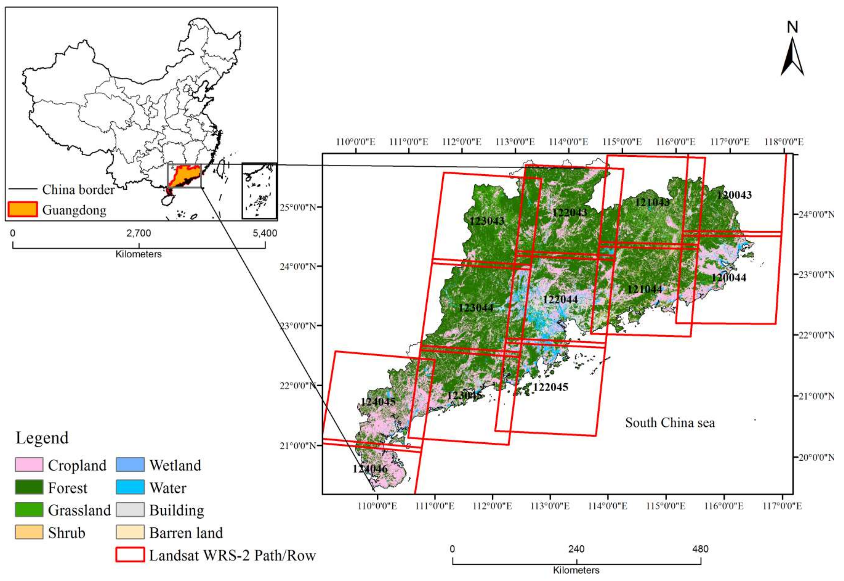
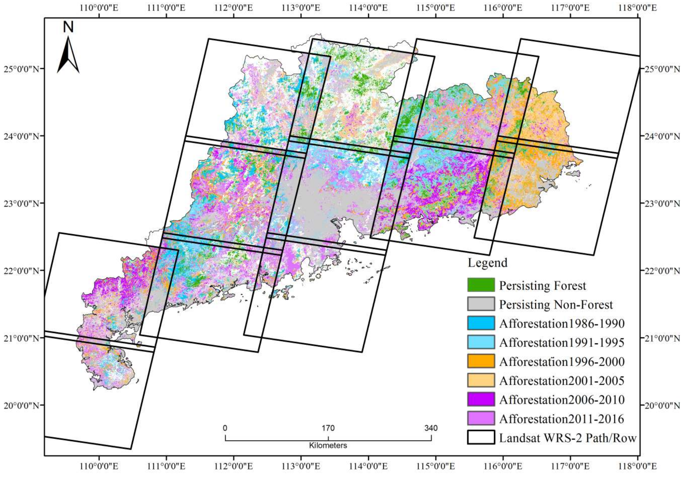
2.1. Study Area
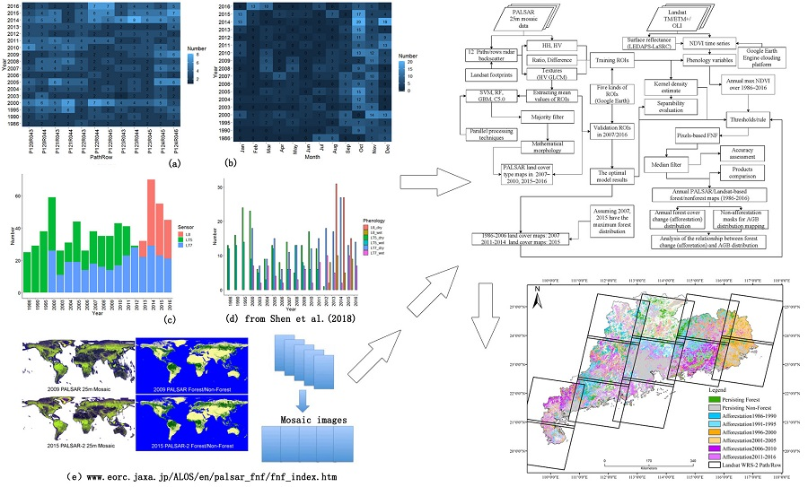
2.2. Active- and Passive-Based Satellite Data
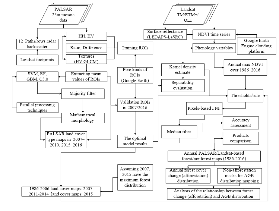
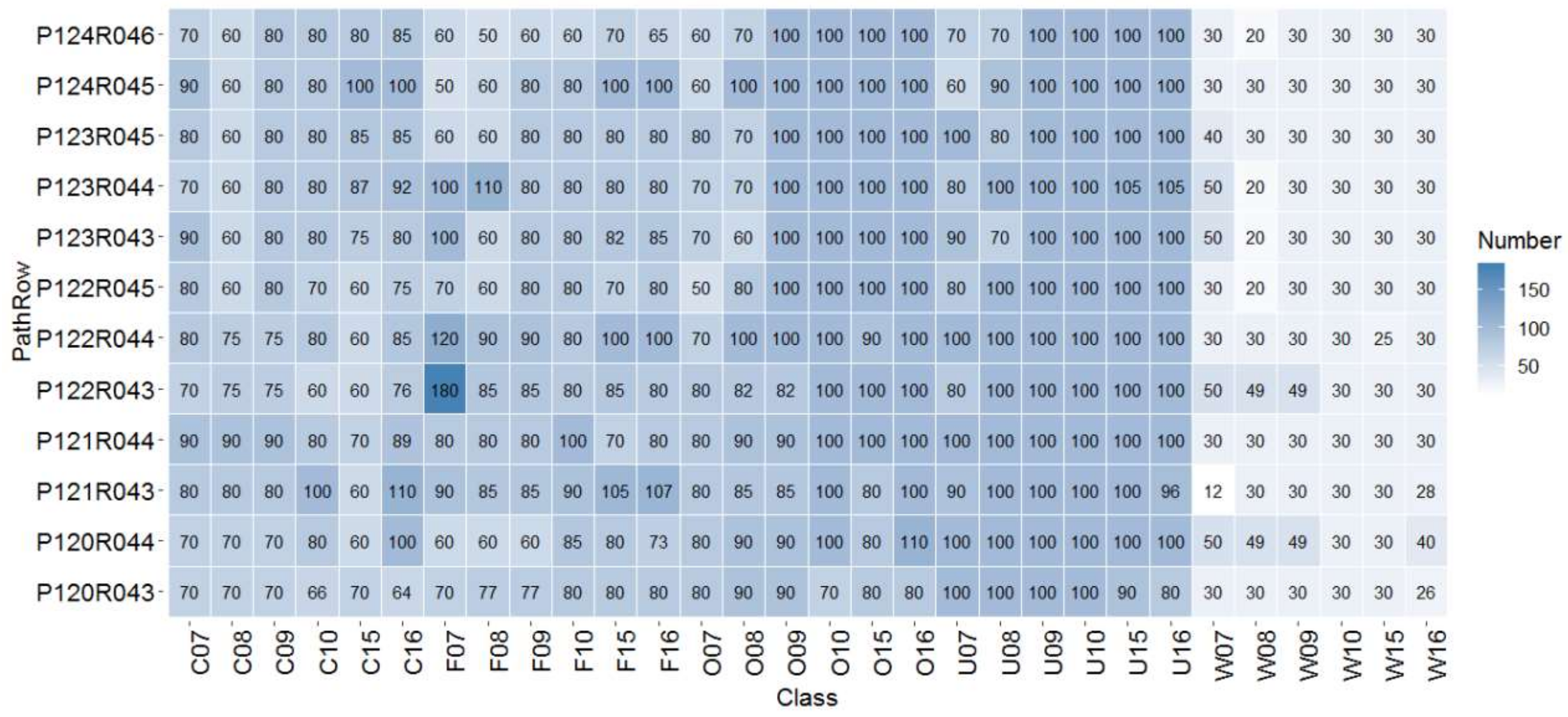
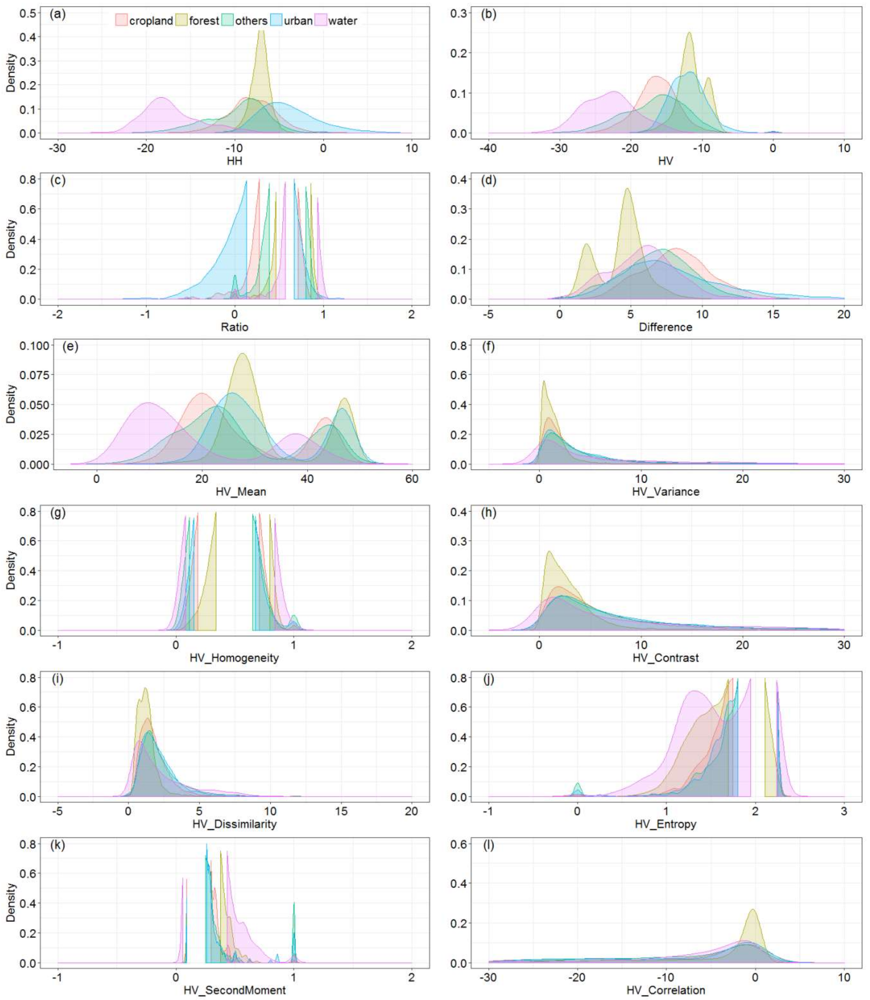
2.3. Extraction of PALSAR Backscatter Signatures for Land Cover Types
2.4. Different Classification Algorithms for Mapping Forest and Non-Forest Based on Multi-Temporal PALSAR
2.4.1. Evaluation of the PALSAR Backscatter Signatures for Land Cover Types
2.4.2. Classification Algorithms
2.4.3. PALSAR-Based Land Cover Types Mapping Assessment
2.5. Mapping the Forest Based on Landsat and PALSAR
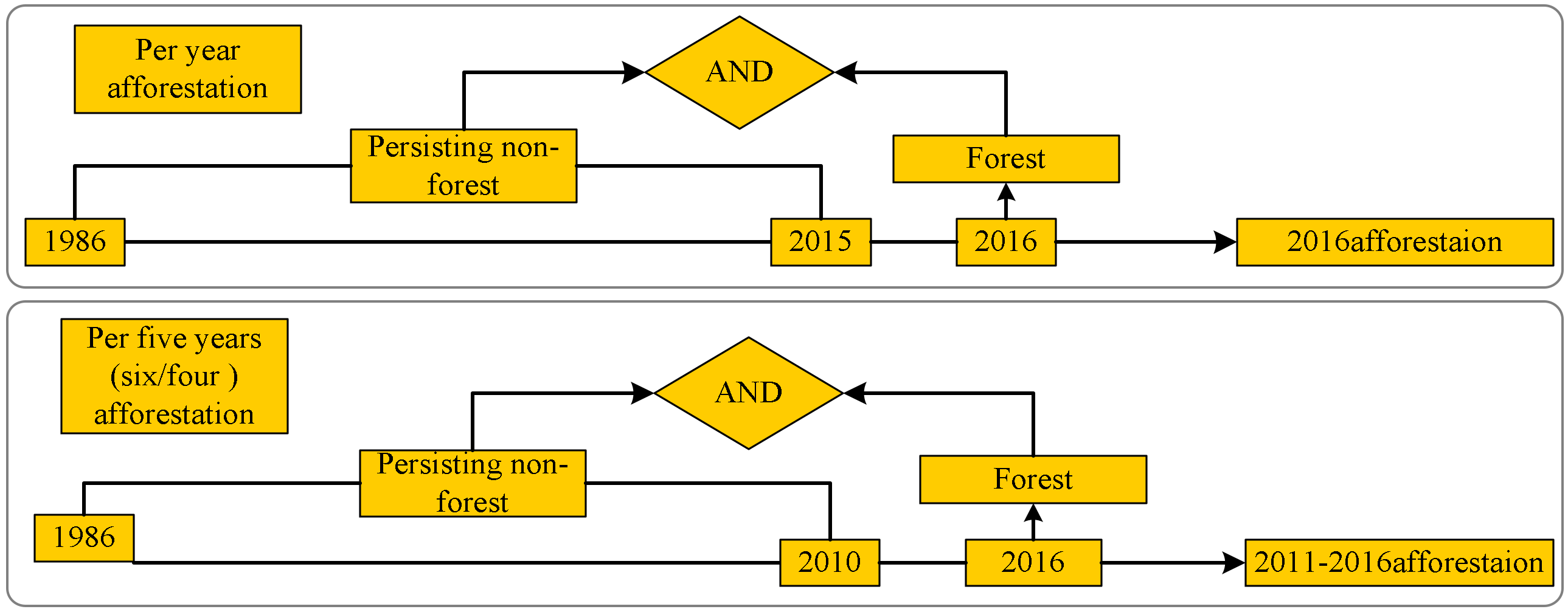
2.5.1. Further Forest Mapping Based on the Integration of PALSAR-Based FNF and Landsat Data
2.5.2. Evaluation of PALSAR/Landsat-Based Forest Maps
2.6. Evaluation of the PALSAR/Landsat-Based Forest Map with Mutlitple Forest Cover Products
2.7. Integration of Forest Aboveground Biomass Change with Annual Forest Cover Changes (Afforestation)
3. Results
3.1. Analysis of Land Cover Types Classification from PALSAR
3.2. Assessment of PALSAR/Landsat-Based Forest/Non-Forest Mapping in Guangdong
3.3. Comparison of the PALSAR/Landsat-Based Forest Map with Other Forest Cover Products
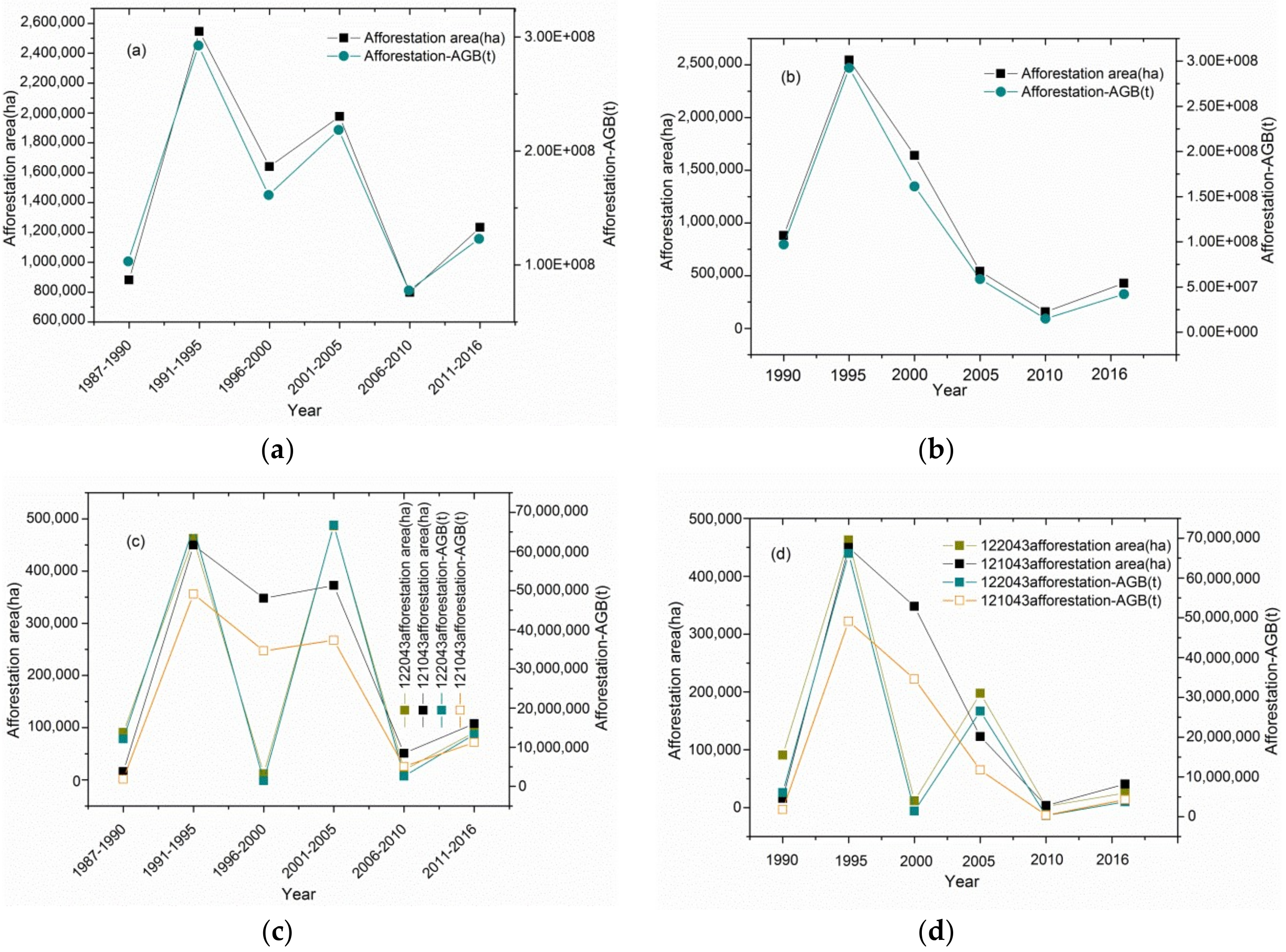
3.4. Relationships Between Forest Cover Change Dynamics (Afforestation) and Forest AGB
4. Discussion
4.1. Extraction of the Spatio-Temporal Dynamics of Forest Cover
4.1.1. Choice of Mapping Algorithms
4.1.2. Comparisons of Forest Cover Maps and the Existing Results
4.2. Forest Cover Dynamics Change Due to Afforestation and Forest AGB
4.3. Uncertainties in the Detection of Forest Change Due to Afforestation
5. Conclusions
Supplementary Materials
Author Contributions
Funding
Acknowledgments
Conflicts of Interest
References
- Zhang, Y.; Liang, S. Changes in forest biomass and linkage to climate and forest disturbances over northeastern china. Glob. Chang. Biol. 2014, 20, 2596–2606. [Google Scholar] [CrossRef] [PubMed]
- Song, X.-P.; Hansen, M.C.; Stehman, S.V.; Potapov, P.V.; Tyukavina, A.; Vermote, E.F.; Townshend, J.R. Global land change from 1982 to 2016. Nature 2018, 560, 639. [Google Scholar] [CrossRef] [PubMed]
- Fang, J.Y.; Chen, A.P.; Peng, C.H.; Zhao, S.Q.; Ci, L. Changes in forest biomass carbon storage in China between 1949 and 1998. Science 2001, 292, 2320–2322. [Google Scholar] [CrossRef] [PubMed]
- Pan, Y.D.; Birdsey, R.A.; Fang, J.Y.; Houghton, R.; Kauppi, P.E.; Kurz, W.A.; Phillips, O.L.; Shvidenko, A.; Lewis, S.L.; Canadell, J.G.; et al. A large and persistent carbon sink in the world’s forests. Science 2011, 333, 988–993. [Google Scholar] [CrossRef] [PubMed]
- Peng, S.S.; Piao, S.; Zeng, Z.; Ciais, P.; Zhou, L.; Li, L.Z.; Myneni, R.B.; Yin, Y.; Zeng, H. Afforestation in china cools local land surface temperature. PNAS 2014, 111, 2915–2919. [Google Scholar] [CrossRef] [PubMed]
- Piao, S.L.; Fang, J.Y.; Ciais, P.; Peylin, P.; Huang, Y.; Sitch, S.; Wang, T. The carbon balance of terrestrial ecosystems in china. Nature 2009, 458, 1009–1013. [Google Scholar] [CrossRef] [PubMed]
- Arora, V.K.; Montenegro, A. Small temperature benefits provided by realistic afforestation efforts. Nat. Geosci. 2011, 4, 514–518. [Google Scholar] [CrossRef]
- Swann, A.L.; Fung, I.Y.; Chiang, J.C. Mid-latitude afforestation shifts general circulation and tropical precipitation. PNAS 2012, 109, 712–716. [Google Scholar] [CrossRef] [PubMed]
- Zeng, W.; Tomppo, E.; Healey, S.P.; Gadow, K.V. The national forest inventory in China: History—Results—International context. For. Ecosyst. 2015, 2, 23. [Google Scholar] [CrossRef]
- Gómez, C.; White, J.C.; Wulder, M.A.; Alejandro, P. Integrated object-based spatiotemporal characterization of forest change from an annual time series of landsat image composites. Can. J. Remote Sens. 2015, 41, 271–292. [Google Scholar] [CrossRef]
- Hansen, M.C.; Potapov, P.V.; Moore, R.; Hancher, M.; Turubanova, S.A.; Tyukavina, A.; Thau, D.; Stehman, S.V.; Goetz, S.J.; Loveland, T.R.; et al. High-resolution global maps of 21st-century forest cover change. Science 2013, 342, 850–853. [Google Scholar] [CrossRef] [PubMed]
- Kim, D.-H.; Sexton, J.O.; Noojipady, P.; Huang, C.; Anand, A.; Channan, S.; Feng, M.; Townshend, J.R. Global, landsat-based forest-cover change from 1990 to 2000. Remote Sens. Environ. 2014, 155, 178–193. [Google Scholar] [CrossRef]
- Townshend, J.R.; Masek, J.G.; Huang, C.Q.; Vermote, E.F.; Gao, F.; Channan, S.; Sexton, J.O.; Feng, M.; Narasimhan, R.; Kim, D.; et al. Global characterization and monitoring of forest cover using landsat data: Opportunities and challenges. Int. J. Digit. Earth 2012, 5, 373–397. [Google Scholar] [CrossRef]
- Coppin, P.; Jonckheere, I.; Nackaerts, K.; Muys, B.; Lambin, E. Digital change detection methods in ecosystem monitoring: A review. Int. J. Remote Sens. 2004, 25, 1565–1596. [Google Scholar] [CrossRef]
- Hansen, M.C.; DeFries, R.S. Detecting long-term global forest change using continuous fields of tree-cover maps from 8-km advanced very high resolution radiometer (AVHRR) data for the years 1982–99. Ecosystems 2004, 7, 695–716. [Google Scholar] [CrossRef]
- Hansen, M.C.; Defries, R.S.; Townshend, J.R.G.; Sohlberg, R. Global land cover classification at 1 km spatial resolution using a classification tree approach. Int. J. Remote Sens. 2000, 21, 1331–1364. [Google Scholar] [CrossRef] [Green Version]
- Hansen, M.C.; Stehman, S.V.; Potapov, P.V. Quantification of global gross forest cover loss. PNAS 2010, 107, 8650–8655. [Google Scholar] [CrossRef] [PubMed] [Green Version]
- Loveland, T.R.; Reed, B.C.; Brown, J.F.; Ohlen, D.O.; Zhu, Z.; Yang, L.; Merchant, J.W. Development of a global land cover characteristics database and igbp discover from 1 km avhrr data. Int. J. Remote Sens. 2000, 21, 1303–1330. [Google Scholar] [CrossRef]
- Chen, J.; Chen, J.; Liao, A.; Cao, X.; Chen, L.; Chen, X.; He, C.; Han, G.; Peng, S.; Lu, M.; et al. Global land cover mapping at 30m resolution: A pok-based operational approach. ISPRS J. Photogramm. 2015, 103, 7–27. [Google Scholar] [CrossRef]
- Gong, P.; Wang, J.; Yu, L.; Zhao, Y.C.; Zhao, Y.Y.; Liang, L.; Niu, Z.G.; Huang, X.M.; Fu, H.H.; Liu, S.; et al. Finer resolution observation and monitoring of global land cover: First mapping results with landsat TM and ETM+ data. Int. J. Remote Sens. 2013, 34, 2607–2654. [Google Scholar] [CrossRef]
- Shimada, M.; Itoh, T.; Motooka, T.; Watanabe, M.; Shiraishi, T.; Thapa, R.; Lucas, R. New global forest/non-forest maps from alos palsar data (2007–2010). Remote Sens. Environ. 2014, 155, 13–31. [Google Scholar] [CrossRef]
- Banskota, A.; Kayastha, N.; Falkowski, M.J.; Wulder, M.A.; Froese, R.E.; White, J.C. Forest monitoring using landsat time series data: A review. Can. J. Remote Sens. 2014, 40, 362–384. [Google Scholar] [CrossRef]
- Huang, C.Q.; Coward, S.N.; Masek, J.G.; Thomas, N.; Zhu, Z.L.; Vogelmann, J.E. An automated approach for reconstructing recent forest disturbance history using dense landsat time series stacks. Remote Sens. Environ. 2010, 114, 183–198. [Google Scholar] [CrossRef]
- Kennedy, R.E.; Yang, Z.; Cohen, W.B. Detecting trends in forest disturbance and recovery using yearly landsat time series: 1. Landtrendr—Temporal segmentation algorithms. Remote Sens. Environ. 2010, 114, 2897–2910. [Google Scholar] [CrossRef]
- Zhu, Z.; Woodcock, C.E. Continuous change detection and classification of land cover using all available landsat data. Remote Sens. Environ. 2014, 144, 152–171. [Google Scholar] [CrossRef]
- Lu, D.; Mausel, P.; Brondizio, E.; Moran, E. Change detection techniques. Int. J. Remote Sens. 2004, 25, 2365–2407. [Google Scholar] [CrossRef]
- Hansen, M.C.; Roy, D.P.; Lindquist, E.; Adusei, B.; Justice, C.O.; Altstatt, A. A method for integrating modis and landsat data for systematic monitoring of forest cover and change in the congo basin. Remote Sens. Environ. 2008, 112, 2495–2513. [Google Scholar] [CrossRef]
- Mitchell, A.L.; Rosenqvist, A.; Mora, B. Current remote sensing approaches to monitoring forest degradation in support of countries measurement, reporting and verification (MRV) systems for redd. Carbon Balance Manag. 2017, 12, 9. [Google Scholar] [CrossRef] [PubMed]
- Reiche, J.; Lucas, R.; Mitchell, A.L.; Verbesselt, J.; Hoekman, D.H.; Haarpaintner, J.; Kellndorfer, J.M.; Rosenqvist, A.; Lehmann, E.A.; Woodcock, C.E.; et al. Combining satellite data for better tropical forest monitoring. Nat. Clim. Chang. 2016, 6, 120. [Google Scholar] [CrossRef]
- Reiche, J.; Verbesselt, J.; Hoekman, D.; Herold, M. Fusing landsat and sar time series to detect deforestation in the tropics. Remote Sens. Environ. 2015, 156, 276–293. [Google Scholar] [CrossRef]
- Sexton, J.O.; Song, X.-P.; Feng, M.; Noojipady, P.; Anand, A.; Huang, C.; Kim, D.-H.; Collins, K.M.; Channan, S.; DiMiceli, C.; et al. Global, 30-m resolution continuous fields of tree cover: Landsat-based rescaling of modis vegetation continuous fields with lidar-based estimates of error. Int. J. Digit. Earth 2013, 6, 427–448. [Google Scholar] [CrossRef]
- Song, X.-P.; Huang, C.; Feng, M.; Sexton, J.O.; Channan, S.; Townshend, J.R. Integrating global land cover products for improved forest cover characterization: An application in north america. Int. J. Digit. Earth 2013, 7, 709–724. [Google Scholar] [CrossRef]
- Wulder, M.A.; White, J.C.; Nelson, R.F.; Næsset, E.; Ørka, H.O.; Coops, N.C.; Hilker, T.; Bater, C.W.; Gobakken, T. Lidar sampling for large-area forest characterization: A review. Remote Sens. Environ. 2012, 121, 196–209. [Google Scholar] [CrossRef] [Green Version]
- Sexton, J.O.; Bax, T.; Siqueira, P.; Swenson, J.J.; Hensley, S. A comparison of lidar, radar, and field measurements of canopy height in pine and hardwood forests of southeastern North America. For. Ecol. Manag. 2009, 257, 1136–1147. [Google Scholar] [CrossRef]
- Reiche, J.; Souzax, C.M.; Hoekman, D.H.; Verbesselt, J.; Persaud, H.; Herold, M. Feature level fusion of multi-temporal alos palsar and landsat data for mapping and monitoring of tropical deforestation and forest degradation. IEEE J. Sel. Top. Appl. Earth Obs. Remote Sens. 2013, 6, 2159–2173. [Google Scholar] [CrossRef]
- Qin, Y.W.; Xiao, X.M.; Wang, J.; Dong, J.W.; Ewing, K.T.; Hoagland, B.; Hough, D.J.; Fagin, T.D.; Zou, Z.H.; Geissler, G.L.; et al. Mapping annual forest cover in sub-humid and semi-arid regions through analysis of landsat and palsar imagery. Remote Sens. 2016, 8, 933. [Google Scholar] [CrossRef]
- De Alban, J.; Connette, G.; Oswald, P.; Webb, E. Combined landsat and L-band sar data improves land cover classification and change detection in dynamic tropical landscapes. Remote Sens. 2018, 10, 306. [Google Scholar] [CrossRef]
- Dong, J.; Xiao, X.; Menarguez, M.A.; Zhang, G.; Qin, Y.; Thau, D.; Biradar, C.; Moore, B., 3rd. Mapping paddy rice planting area in northeastern asia with landsat 8 images, phenology-based algorithm and google earth engine. Remote Sens. Environ. 2016, 185, 142–154. [Google Scholar] [CrossRef] [PubMed]
- Lehmann, E.A.; Wallace, J.F.; Caccetta, P.A.; Furby, S.L.; Zdunic, K. Forest cover trends from time series landsat data for the australian continent. Int. J. Appl. Earth Obs. Geoinf. 2013, 21, 453–462. [Google Scholar] [CrossRef]
- Walker, W.S.; Stickler, C.M.; Kellndorfer, J.M.; Kirsch, K.M.; Nepstad, D.C. Large-area classification and mapping of forest and land cover in the brazilian amazon: A comparative analysis of alos/palsar and landsat data sources. IEEE J. Sel. Top. Appl. Earth Obs. Remote Sens. 2010, 3, 594–604. [Google Scholar] [CrossRef]
- Sirro, L.; Häme, T.; Rauste, Y.; Kilpi, J.; Hämäläinen, J.; Gunia, K.; de Jong, B.; Paz Pellat, F. Potential of different optical and sar data in forest and land cover classification to support REDD+ MRV. Remote Sens. 2018, 10, 942. [Google Scholar] [CrossRef]
- Wang, J.; Xiao, X.; Qin, Y.; Dong, J.; Geissler, G.; Zhang, G.; Cejda, N.; Alikhani, B.; Doughty, R.B. Mapping the dynamics of eastern redcedar encroachment into grasslands during 1984–2010 through palsar and time series landsat images. Remote Sens. Environ. 2017, 190, 233–246. [Google Scholar] [CrossRef]
- Wang, J.; Xiao, X.; Qin, Y.; Doughty, R.B.; Dong, J.; Zou, Z. Characterizing the encroachment of juniper forests into sub-humid and semi-arid prairies from 1984 to 2010 using palsar and landsat data. Remote Sens. Environ. 2018, 205, 166–179. [Google Scholar] [CrossRef]
- Bauer, E.; Kohavi, R. An empirical comparison of voting classification algorithms: Bagging, boosting, and variants. Mach. Learn. 1998, pp. 1–38. Available online: http://citeseerx.ist.psu.edu/viewdoc/download?doi=10.1.1.50.6504&rep=rep1&type=pdf (accessed on 31 January 2019).
- Huang, C.; Davis, L.S.; Townshend, J.R.G. An assessment of support vector machines for land cover classification. Int. J. Remote Sens. 2002, 23, 725–749. [Google Scholar] [CrossRef]
- Pandya, R.; Pandya, J. C5. 0 algorithm to improved decision tree with feature selection and reduced error pruning. Int. J. Comput. Appl. 2015, 117, 18–21. [Google Scholar] [CrossRef]
- Chirici, G.; Scotti, R.; Montaghi, A.; Barbati, A.; Cartisano, R.; Lopez, G.; Marchetti, M.; McRoberts, R.E.; Olsson, H.; Corona, P. Stochastic gradient boosting classification trees for forest fuel types mapping through airborne laser scanning and irs liss-iii imagery. Int. J. Appl. Earth Obs. Geoinf. 2013, 25, 87–97. [Google Scholar] [CrossRef]
- Lawrence, R. Classification of remotely sensed imagery using stochastic gradient boosting as a refinement of classification tree analysis. Remote Sens. Environ. 2004, 90, 331–336. [Google Scholar] [CrossRef]
- Moisen, G.G.; Freeman, E.A.; Blackard, J.A.; Frescino, T.S.; Zimmermann, N.E.; Edwards, T.C. Predicting tree species presence and basal area in Utah: A comparison of stochastic gradient boosting, generalized additive models, and tree-based methods. Ecol. Model. 2006, 199, 176–187. [Google Scholar] [CrossRef]
- Baker, C.; Lawrence, R.; Montagne, C.; Patten, D. Mapping wetlands and riparian areas using landsat ETM+ imagery and decision-tree-based models. Wetlands 2006, 26, 465–474. [Google Scholar] [CrossRef]
- Dong, J.; Xiao, X.; Sheldon, S.; Biradar, C.; Duong, N.D.; Hazarika, M. A comparison of forest cover maps in mainland southeast asia from multiple sources: Palsar, meris, modis and FRA. Remote Sens. Environ. 2012, 127, 60–73. [Google Scholar] [CrossRef]
- Qin, Y.; Xiao, X.; Dong, J.; Zhang, G.; Roy, P.S.; Joshi, P.K.; Gilani, H.; Murthy, M.S.; Jin, C.; Wang, J.; et al. Mapping forests in monsoon asia with alos palsar 50-m mosaic images and modis imagery in 2010. Sci. Rep. 2016, 6, 20880. [Google Scholar] [CrossRef] [PubMed]
- Pastor-Guzman, J.; Dash, J.; Atkinson, P.M. Remote sensing of mangrove forest phenology and its environmental drivers. Remote Sens. Environ. 2018, 205, 71–84. [Google Scholar] [CrossRef]
- Prabakaran, C.; Singh, C.P.; Panigrahy, S.; Parihar, J.S. Retrieval of forest phenological parameters from remote sensing-based NDVI time-series data. Curr. Sci. India 2013, 105, 795–802. [Google Scholar]
- Brown, S.; Lugo, A.E.; Chapman, J.D. Biomass of tropical tree plantation and its implications for the global carbon budget. Can. J. For. Res. 1986, 16, 390–394. [Google Scholar] [CrossRef]
- Wang, H.; Mo, J.; Lu, X.; Xue, J.; Li, J.; Fang, Y. Effects of elevated nitrogen deposition on soil microbial biomass carbon in major subtropical forests of southern china. Front. For. China 2009, 4, 21–27. [Google Scholar] [CrossRef]
- Shen, W.J.; Li, M.S.; Huang, C.Q.; Wei, A.S. Quantifying live aboveground biomass and forest disturbance of mountainous natural and plantation forests in northern guangdong, china, based on multi-temporal landsat, palsar and field plot data. Remote Sens. 2016, 8, 595. [Google Scholar] [CrossRef]
- Shen, W.; Li, M.; Huang, C.; Tao, X.; Wei, A. Annual forest aboveground biomass changes mapped using icesat/glas measurements, historical inventory data, and time-series optical and radar imagery for guangdong province, China. Agric. For. Meteorol. 2018, 259, 23–38. [Google Scholar] [CrossRef]
- Silverman, B.W. Density Estimation for Statistics and Data Analysis; CRC Press: Boca Raton, FL, USA, 1986. [Google Scholar]
- R Development Core Team. R: A Language and Environment for Statistical Computing; R Foundation for Statistical Computing: Vienna, Austria, 2008. [Google Scholar]
- Ridgeway, G. Generalized boosted models: A guide to the gbm package. Update 2007, 1, 2007. [Google Scholar]
- Weston, S.; Calaway, R. Getting started with doparallel and foreach. Data Access 2017, 30. Available online: ftp://expo.lcs.mit.edu/pub/CRAN/web/packages/doParallel/vignettes/gettingstartedParallel.pdf (accessed on 31 January 2019).
- Leon, T.; Ayala, G.; Gaston, M.; Mallor, F. Using mathematical morphology for unsupervised classification of functional data. J. Stat. Comput. Simul. 2011, 81, 1001–1016. [Google Scholar] [CrossRef]
- Thenkabail, P.S.; Schull, M.; Turral, H. Ganges and indus river basin land use/land cover (LULC) and irrigated area mapping using continuous streams of modis data. Remote Sens. Environ. 2005, 95, 317–341. [Google Scholar] [CrossRef]
- Simard, M.; Saatchi, S.S.; De Grandi, G. The use of decision tree and multiscale texture for classification of JERS-1 SAR data over tropical forest. IEEE Trans. Geosci. Remote Sens. 2000, 38, 2310–2321. [Google Scholar] [CrossRef] [Green Version]
- Meyer, F.J.; Chotoo, K.; Chotoo, S.D.; Huxtable, B.D.; Carrano, C.S. The influence of equatorial scintillation on L-band SAR image quality and phase. IEEE Trans. Geosci. Remote Sens. 2016, 54, 869–880. [Google Scholar] [CrossRef]
- Santoro, M.; Fransson, J.E.S.; Eriksson, L.E.B.; Magnusson, M.; Ulander, L.M.H.; Olsson, H. Signatures of alos palsar L-band backscatter in Swedish forest. IEEE Trans. Geosci. Remote Sens. 2009, 47, 4001–4019. [Google Scholar] [CrossRef]
- Abdikan, S.; Bayik, C. Assessment of alos palsar 25-m mosaic data for land cover mapping. In Proceedings of the 2017 9th International Workshop on the Analysis of Multitemporal Remote Sensing Images (MultiTemp), Brugge, Belgium, 27–29 June 2017; pp. 1–4. [Google Scholar]
- Freeman, E.D.; Larsen, R.T.; Peterson, M.E.; Anderson, C.R.; Hersey, K.R.; Mcmillan, B.R. Effects of male-biased harvest on mule deer: Implications for rates of pregnancy, synchrony, and timing of parturition. Wildl. Soc. B 2014, 38, 806–811. [Google Scholar] [CrossRef]
- Chen, B.; Xiao, X.; Ye, H.; Ma, J.; Doughty, R.; Li, X.; Zhao, B.; Wu, Z.; Sun, R.; Dong, J.; et al. Mapping forest and their spatial–temporal changes from 2007 to 2015 in tropical hainan island by integrating ALOS/ALOS-2 L-band SAR and landsat optical images. IEEE J. Sel. Top. Appl. Earth Obs. Remote Sens. 2018, 11, 852–867. [Google Scholar] [CrossRef]
- Altese, E.; Bolognani, O.; Mancini, M.; Troch, P.A. Retrieving soil moisture over bare soil from ers 1 synthetic aperture radar data: Sensitivity analysis based on a theoretical surface scattering model and field data. Water Resour. Res. 1996, 32, 653–661. [Google Scholar] [CrossRef]
- Huete, A.; Didan, K.; Miura, T.; Rodriguez, E.P.; Gao, X.; Ferreira, L.G. Overview of the radiometric and biophysical performance of the modis vegetation indices. Remote Sens. Environ. 2002, 83, 195–213. [Google Scholar] [CrossRef]
- Xiao, X.; Hagen, S.; Zhang, Q.; Keller, M.; Moore, B. Detecting leaf phenology of seasonally moist tropical forests in south america with multi-temporal modis images. Remote Sens. Environ. 2006, 103, 465–473. [Google Scholar] [CrossRef]
- Zhang, X. Reconstruction of a complete global time series of daily vegetation index trajectory from long-term AVHRR data. Remote Sens. Environ. 2015, 156, 457–472. [Google Scholar] [CrossRef]
- Healey, S.P.; Patterson, P.L.; Saatchi, S.; Lefsky, M.A.; Lister, A.J.; Freeman, E.A. A sample design for globally consistent biomass estimation using lidar data from the geoscience laser altimeter system (GLAS). Carbon Balance Manag. 2012, 7, 1–10. [Google Scholar] [CrossRef] [PubMed]
- Fritz, S.; See, L. Identifying and quantifying uncertainty and spatial disagreement in the comparison of global land cover for different applications. Glob. Chang. Biol. 2008, 14, 1057–1075. [Google Scholar] [CrossRef]
- Lu, D.; Weng, Q. A survey of image classification methods and techniques for improving classification performance. Int. J. Remote Sens. 2007, 28, 823–870. [Google Scholar] [CrossRef] [Green Version]
- Olofsson, P.; Foody, G.M.; Stehman, S.V.; Woodcock, C.E. Making better use of accuracy data in land change studies: Estimating accuracy and area and quantifying uncertainty using stratified estimation. Remote Sens. Environ. 2013, 129, 122–131. [Google Scholar] [CrossRef]
- Wulder, M.A.; Coops, N.C.; Roy, D.P.; White, J.C.; Hermosilla, T. Land cover 2.0. Int. J. Remote Sens. 2018, 39, 4254–4284. [Google Scholar] [CrossRef] [Green Version]
- Nemani, R.; Votava, P.; Michaelis, A.; Melton, F.; Milesi, C. Collaborative supercomputing for global change science. Eos Trans. Am. Geophys. Union 2011, 92, 109–110. [Google Scholar] [CrossRef]


| Sensor | Date | Resolution | Techniques | Derivatives | Reference |
|---|---|---|---|---|---|
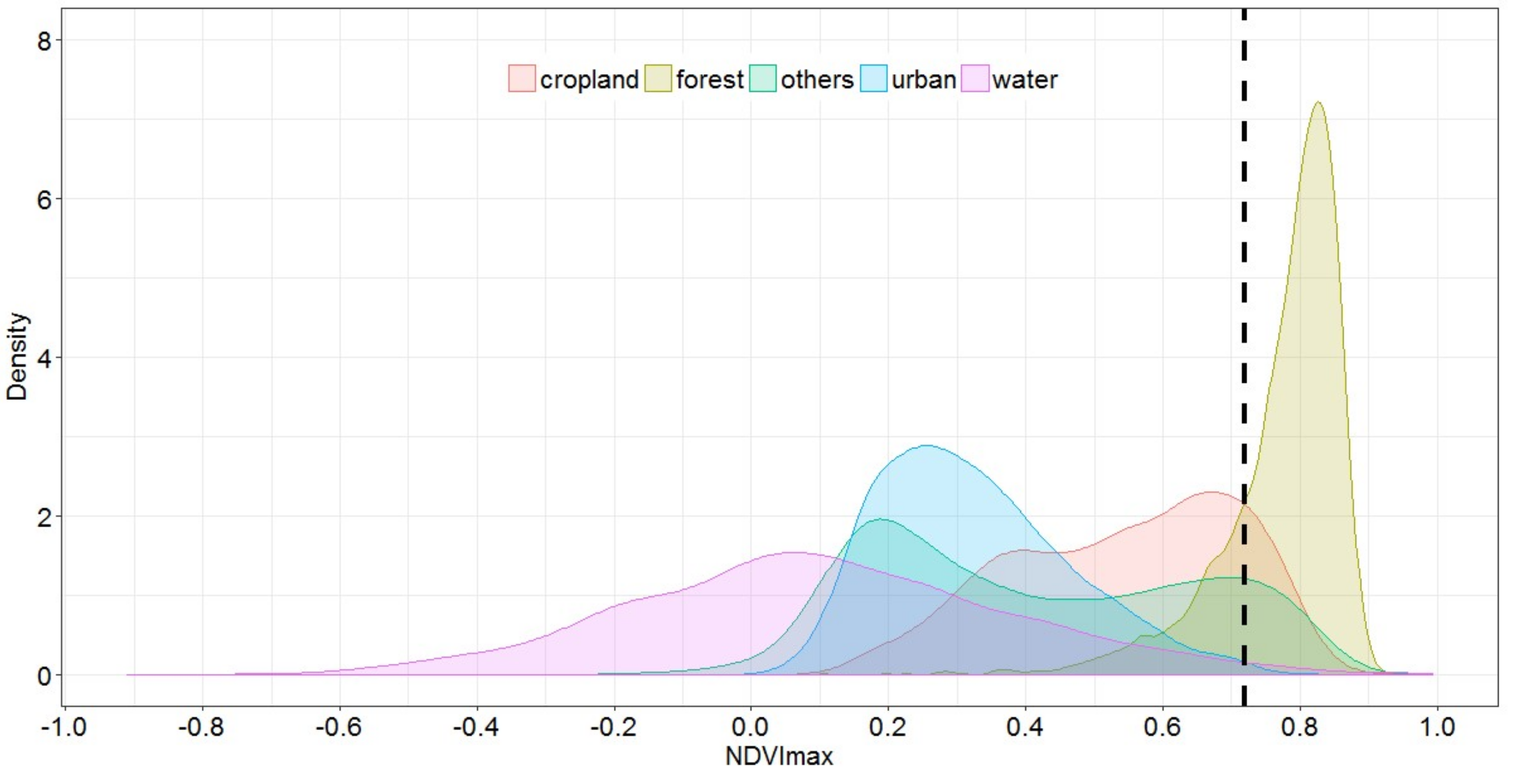
| Landsat 5&7& 8 | 1986–2016 | 30 m | Google Earth Engine | Cumulative time-series maximum normalized difference vegetation index (NDVI) in dry and wet season | [58] |
| PALSAR mosaic | 2007–2010, 2015–2016 (Jul–Sep) | 25 m | Parallel processing | HH, HV, HV texture measures (mean, variance, homogeneity, contrast, dissimilarity, entropy, second moment, and correlation), HH/HV (ratio), HH-HV (difference) |
| Classifiers | Implementation | Parameters | Packages |
|---|---|---|---|
| SVM | R studio | kernel: RBF (radial basis function) gamma:1 cost:1 type: C-classification | e1071 |
| RF | R studio | ntree = 500 Importance = TRUE | randomForest |
| GBM | R studio | n.trees = 3000 shrinkage = 0.01 | gbm |
| C5.0 | R studio | trials = 10 | C50 |
| Products | Resolution | Forest Definition | Algorithms | References |
|---|---|---|---|---|
| GLC30 | 30 m | Canopy cover over 30% (including sparse woods over 10–30%) | MLC+Expert interpretation | [19] |
| VCT | 30 m | Pixels having low IFZ value near 0 are close to the spectral center of forest samples | Integrated forest z-score (IFZ) | [23] |
| PALSAR FNF | 25 m | canopy cover over 10%, and the area must be larger than 0.5 ha | Backscatter thresholds | [21] |
| PALSAR/Landsat-based FNF (this study) | 30 m | canopy cover over 10% | Classifiers+NDVImax |
| Year | Class | Producer Accuracy (%) | User Accuracy (%) | Overall Accuracy/Kappa Coefficient |
|---|---|---|---|---|
| 2005 | F | 77.66% | 51.56% | 76.89% (95% CI:75.11%–78.6%)/0.463 |
| NF | 76.64% | 91.47% | ||
| 2010 | F | 71.81% | 61.49% | 84.75 % (95% CI: 83.28%–86.2%)/0.565 |
| NF | 88.16% | 92.24% | ||
| 2016 | F | 85.53% | 57.09% | 83.39% (95% CI: 81.9%–84.81%)/0.578 |
| NF | 82.82% | 95.54% |
| Product | Class | Producer Accuracy (%) | User Accuracy (%) | Overall Accuracy/Kappa Coefficient |
|---|---|---|---|---|
| GLC30 (GD) | F | 89.73% | 60.56% | 85.75 % (95% CI: 84.31–87.11%)/0.633 |
| NF | 84.71% | 96.9% | ||
| JAXA (GD) | F | 71.32% | 52.87% | 80.74% (95 % CI: 79.13–82.27%)/0.483 |
| NF | 83.22% | 91.66% | ||
| This study (p122r043) | F | 92.86% | 55.32% | 86.14% (95% CI: 79.94–91.01%)/0.611 |
| NF | 84.78% | 98.32% | ||
| VCT (p122r043) | F | 92.86% | 65.0% | 90.3% (95% CI: 84.82–94.39%)/0.707 |
| NF | 89.86% | 98.41% |
© 2019 by the authors. Licensee MDPI, Basel, Switzerland. This article is an open access article distributed under the terms and conditions of the Creative Commons Attribution (CC BY) license (http://creativecommons.org/licenses/by/4.0/).
Share and Cite
Shen, W.; Li, M.; Huang, C.; Tao, X.; Li, S.; Wei, A. Mapping Annual Forest Change Due to Afforestation in Guangdong Province of China Using Active and Passive Remote Sensing Data. Remote Sens. 2019, 11, 490. https://doi.org/10.3390/rs11050490
Shen W, Li M, Huang C, Tao X, Li S, Wei A. Mapping Annual Forest Change Due to Afforestation in Guangdong Province of China Using Active and Passive Remote Sensing Data. Remote Sensing. 2019; 11(5):490. https://doi.org/10.3390/rs11050490
Chicago/Turabian StyleShen, Wenjuan, Mingshi Li, Chengquan Huang, Xin Tao, Shu Li, and Anshi Wei. 2019. "Mapping Annual Forest Change Due to Afforestation in Guangdong Province of China Using Active and Passive Remote Sensing Data" Remote Sensing 11, no. 5: 490. https://doi.org/10.3390/rs11050490