Evaluation of Using Sentinel-1 and -2 Time-Series to Identify Winter Land Use in Agricultural Landscapes

Abstract
:1. Introduction
2. Study Site and Data
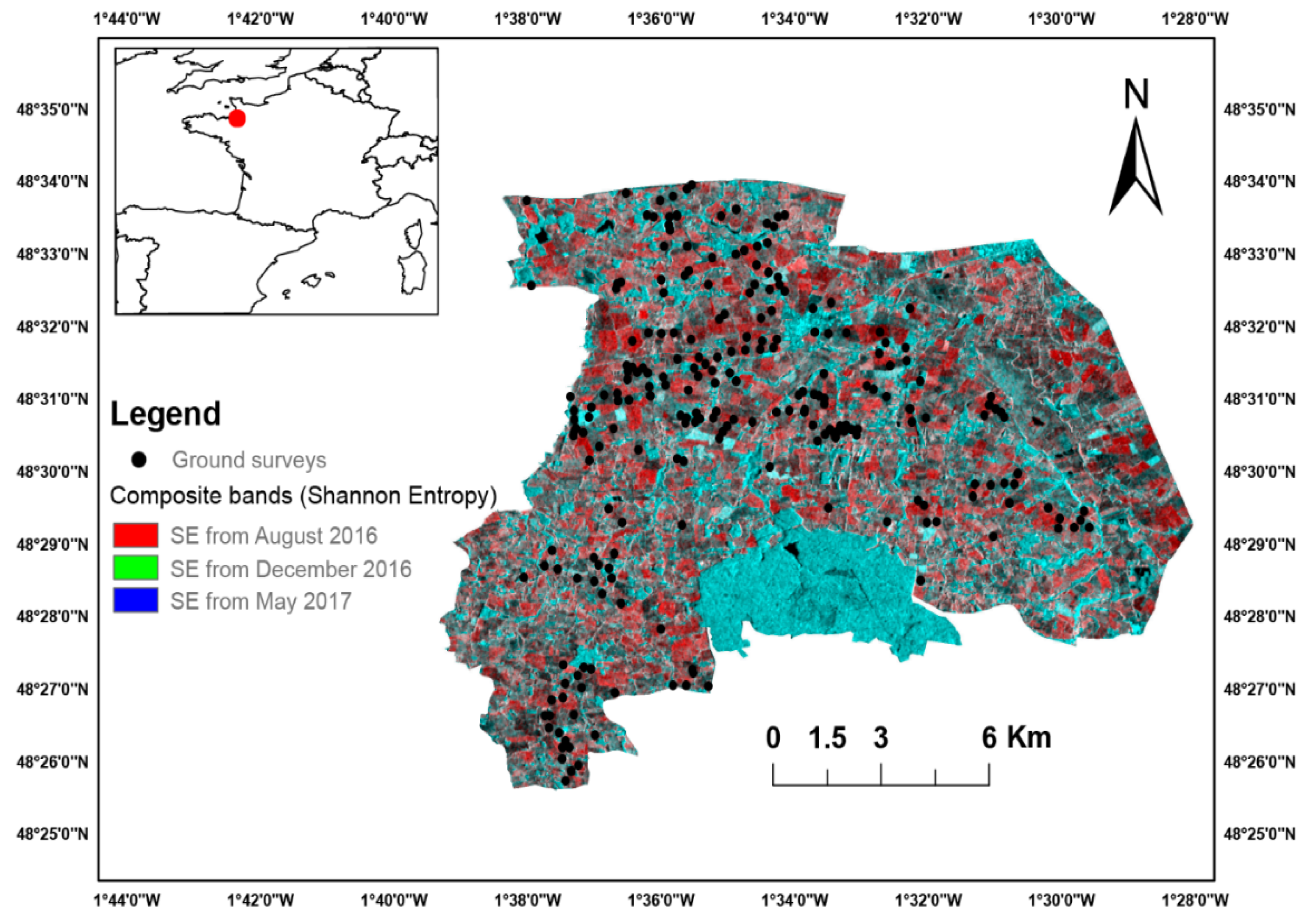
2.1. Study Site
2.2. Field Data
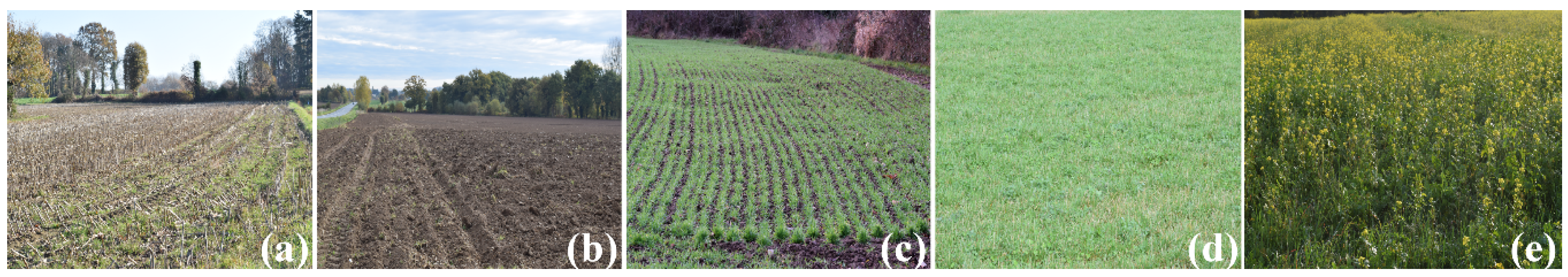
Land Use Data
2.3. Satellite Imagery
3. Materials and Methods
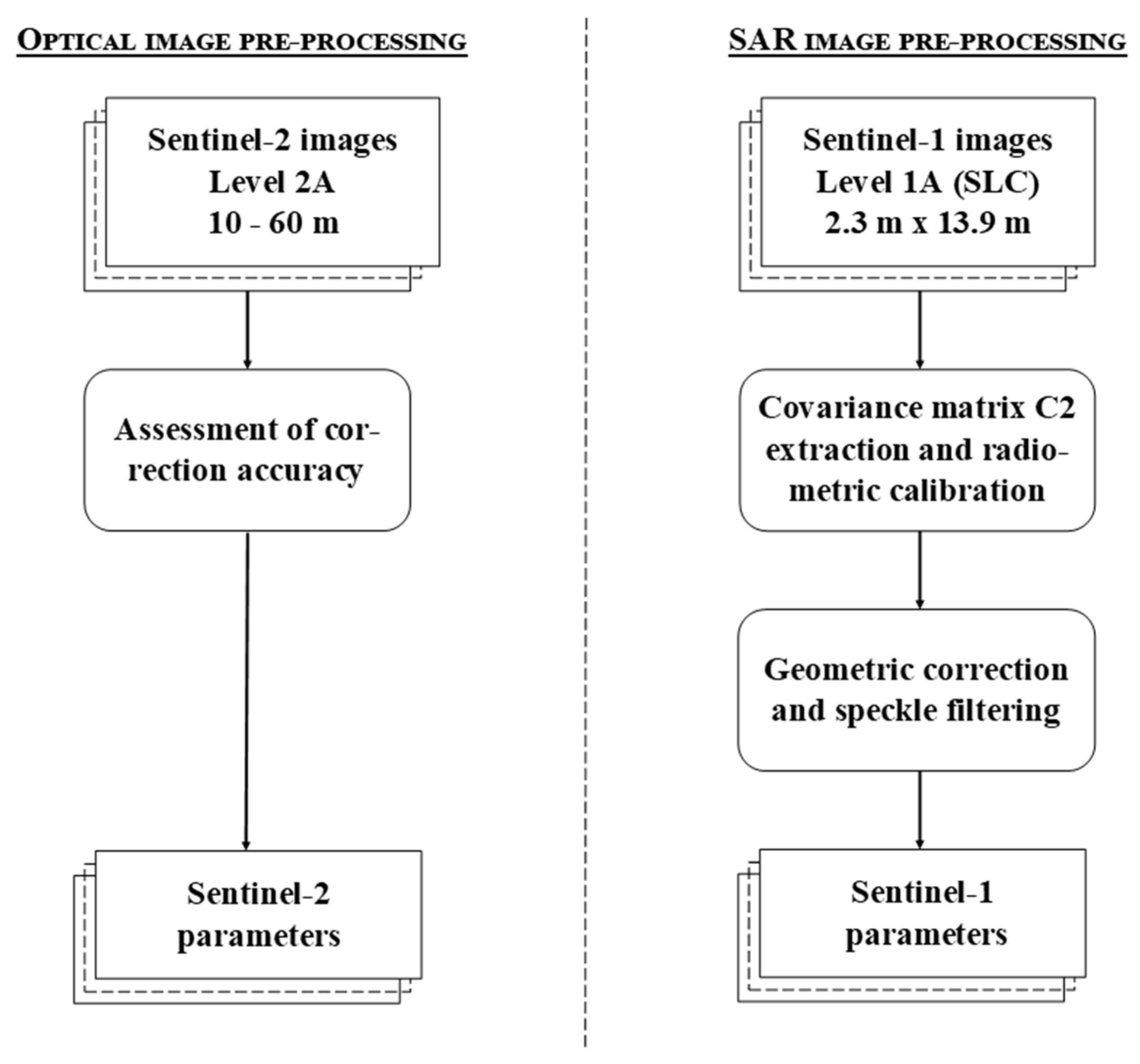
3.1. Pre-Processing of Time-Series
3.1.1. Pre-processing of Sentinel-1 Images
Backscattering Coefficients
Polarimetric Parameters
3.1.2. Pre-processing of Sentinel-2 Images
Calculation of Vegetation Indices and Biophysical Parameters
3.2. Processing Sentinel-1 and -2 Time-Series
3.2.1. Feature Extraction
3.2.2. Reduction of the Parameter Dataset
3.2.3. Land Use Classification
4. Results and Discussion
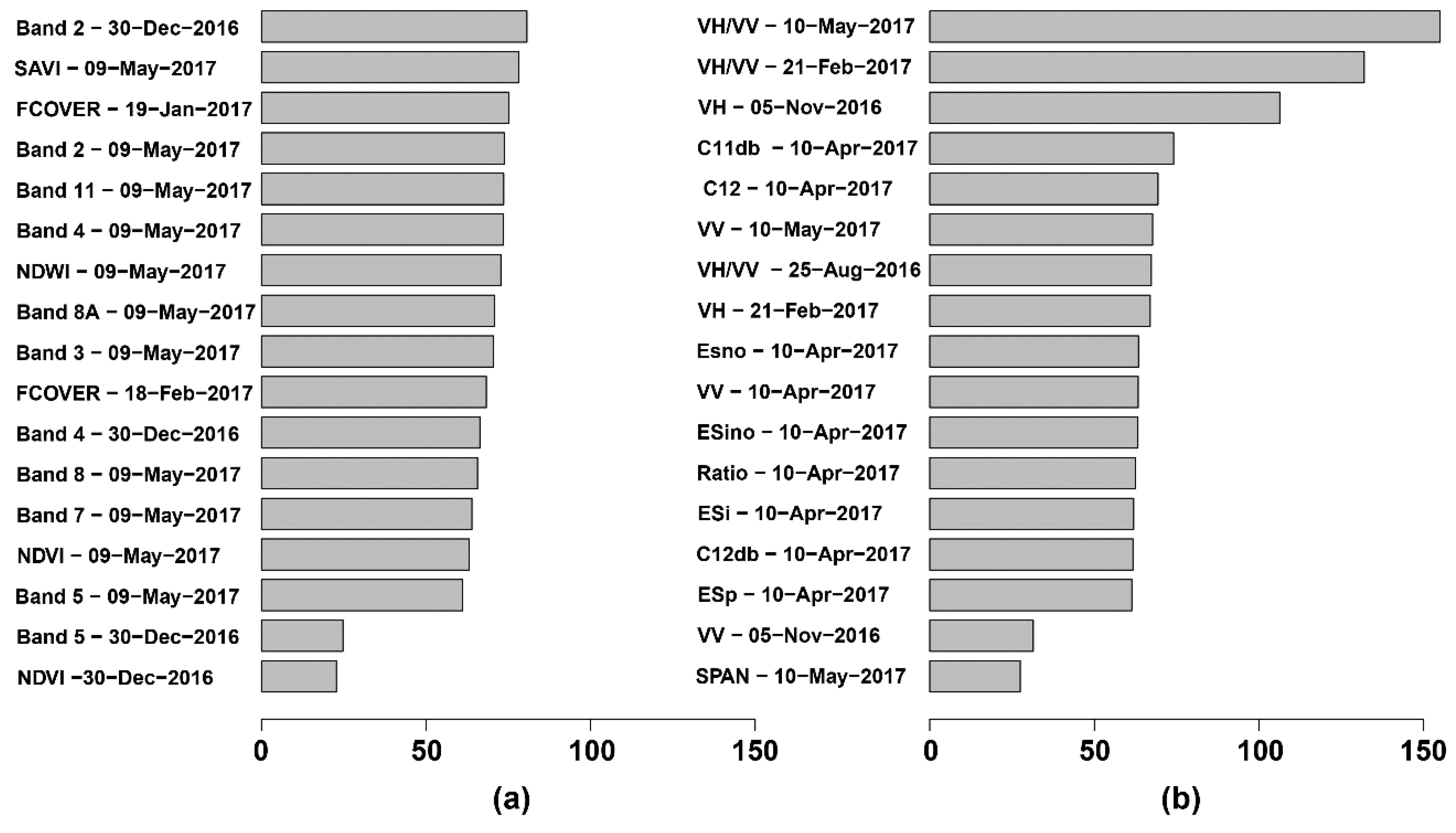
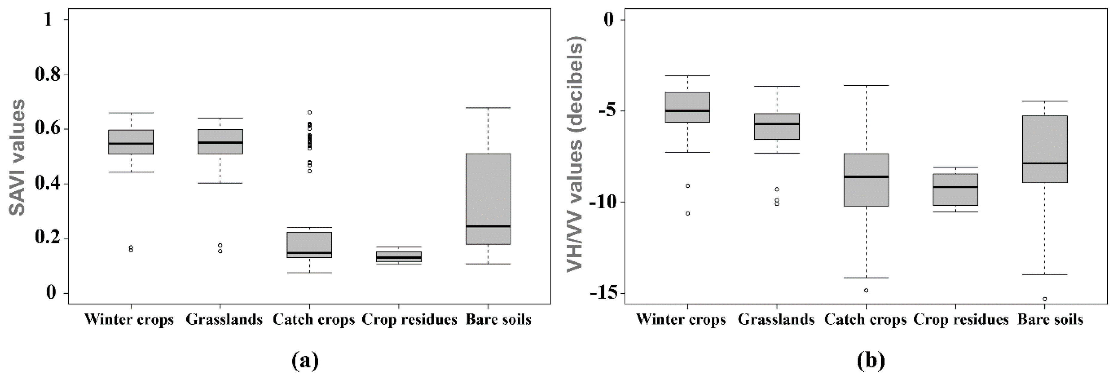
4.1. Importance of Optical and SAR Parameters for Identifying Winter Land Use
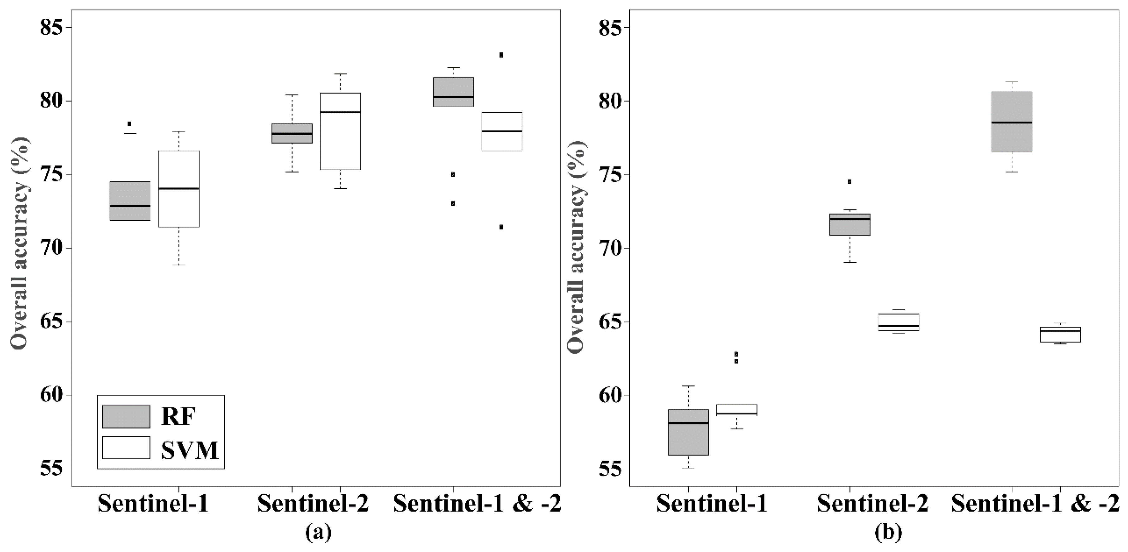
4.2. Winter Land Use Classification
5. Conclusions
Author Contributions
Funding
Acknowledgments
References
- Withers, P.J.; Neal, C.; Jarvie, H.P.; Doody, D.G. Agriculture and Eutrophication: Where Do We Go from Here? Sustainability 2014, 6, 5853–5875. [Google Scholar] [CrossRef] [Green Version]
- Galloway, J.N.; Townsend, A.R.; Erisman, J.W.; Bekunda, M.; Cai, Z.; Freney, J.R.; Martinelli, L.A.; Seitzinger, S.P.; Sutton, M.A. Transformation of the Nitrogen Cycle: Recent Trends, Questions, and Potential Solutions. Science 2008, 320, 889–892. [Google Scholar] [CrossRef] [PubMed] [Green Version]
- Dabney, S.M. Cover Crop Impacts on Watershed Hydrology. J. Soil Water Conserv. 1998, 53, 207–213. [Google Scholar]
- Corgne, S. Hiérarchisation Des Facteurs Structurant Les Dynamiques Pluriannuelles Des Sols Nus Hivernaux. Application Au Bassin Versant Du Yar (Bretagne). Norois. Environ. Aménage. Soc. 2004, 193, 17–29. [Google Scholar] [CrossRef]
- Fieuzal, R.; Baup, F.; Marais-Sicre, C. Monitoring Wheat and Rapeseed by Using Synchronous Optical and Radar Satellite Data—From Temporal Signatures to Crop Parameters Estimation. Adv. Remote Sens. 2013, 2013. [Google Scholar] [CrossRef]
- Zhang, X.; Friedl, M.A.; Schaaf, C.B.; Strahler, A.H.; Hodges, J.C.F.; Gao, F.; Reed, B.C.; Huete, A. Monitoring Vegetation Phenology Using MODIS. Remote Sens. Environ. 2003, 84, 471–475. [Google Scholar] [CrossRef]
- Clark, M.L.; Aide, T.M.; Grau, H.R.; Riner, G. A Scalable Approach to Mapping Annual Land Cover at 250 M Using MODIS Time Series Data: A Case Study in the Dry Chaco Ecoregion of South America. Remote Sens. Environ. 2010, 114, 2816–2832. [Google Scholar] [CrossRef]
- Lecerf, R.; Hubert-Moy, L.; Corpetti, T.; Baret, F.; Latif, B.A.; Nicolas, H. Estimating Biophysical Variables at 250 M with Reconstructed EOS/MODIS Time Series to Monitor Fragmented Landscapes. In Proceedings of the IEEE International Geoscience and Remote Sensing Symposium, Boston, MA, USA, 7–11 July 2008; Volume 2. [Google Scholar] [CrossRef]
- Hubert-Moy, L.; Lecerf, R.; Corpetti, T.; Dubreuil, V. Monitoring Winter Vegetation Cover Using Multitemporal Modis Data. In Proceedings of the IEEE International Conference on Geoscience and Remote Sensing Symposium (IGARSS’05), Seoul, South Korea, 29 July 2005; Volume 3, pp. 2113–2116. [Google Scholar]
- Lecerf, R.; Corpetti, T.; Hubert-Moy, L.; Dubreuil, V. Monitoring Land Use and Land Cover Changes in Oceanic and Fragmented Landscapes with Reconstructed MODIS Time Series. In Proceedings of the International Workshop on the Analysis of Multi-Temporal Remote Sensing Images, Biloxi, MS, USA, 16–18 May 2005; pp. 195–199. [Google Scholar]
- Xu, D. Compare NDVI Extracted from Landsat 8 Imagery with That from Landsat 7 Imagery. Am. J. Remote Sens. 2014, 2, 10. [Google Scholar] [CrossRef]
- Pan, Z.; Huang, J.; Zhou, Q.; Wang, L.; Cheng, Y.; Zhang, H.; Blackburn, G.A.; Yan, J.; Liu, J. Mapping Crop Phenology Using NDVI Time-Series Derived from HJ-1 A/B Data. Int. J. Appl. Earth Observ. Geoinf. 2015, 34, 188–197. [Google Scholar] [CrossRef]
- El Hajj, M.; Bégué, A.; Guillaume, S.; Martiné, J.-F. Integrating SPOT-5 Time Series, Crop Growth Modeling and Expert Knowledge for Monitoring Agricultural practices—The Case of Sugarcane Harvest on Reunion Island. Remote Sens. Environ. 2009, 113, 2052–2061. [Google Scholar] [CrossRef]
- Murakami, T.; Ogawa, S.; Ishitsuka, N.; Kumagai, K.; Saito, G. Crop Discrimination with Multitemporal SPOT/HRV Data in the Saga Plains, Japan. Int. J. Remote Sens. 2001, 22, 1335–1348. [Google Scholar] [CrossRef]
- Bannari, A.; Pacheco, A.; Staenz, K.; McNairn, H.; Omari, K. Estimating and Mapping Crop Residues Cover on Agricultural Lands Using Hyperspectral and IKONOS Data. Remote Sens. Environ. 2006, 104, 447–459. [Google Scholar] [CrossRef]
- Pacheco, A.; McNairn, H. Evaluating Multispectral Remote Sensing and Spectral Unmixing Analysis for Crop Residue Mapping. Remote Sens. Environ. 2010, 114, 2219–2228. [Google Scholar] [CrossRef]
- McNairn, H.; Brisco, B. The Application of C-Band Polarimetric SAR for Agriculture: A Review. Can. J. Remote Sens. 2004, 30, 525–542. [Google Scholar] [CrossRef]
- Smith, L.C. Satellite Remote Sensing of River Inundation Area, Stage, and Discharge: A Review. Hydrol. Process. 1997, 11, 1427–1439. [Google Scholar] [CrossRef]
- Betbeder, J.; Rapinel, S.; Corgne, S.; Pottier, E.; Hubert-Moy, L. TerraSAR-X Dual-Pol Time-Series for Mapping of Wetland Vegetation. ISPRS J. Photogramm. Remote Sens. 2015, 107, 90–98. [Google Scholar] [CrossRef]
- McNairn, H.; Duguay, C.; Boisvert, J.; Huffman, E.; Brisco, B. Defining the Sensitivity of Multi-Frequency and Multi-Polarized Radar Backscatter to Post-Harvest Crop Residue. Can. J. Remote Sens. 2001, 27, 247–263. [Google Scholar] [CrossRef]
- Baghdadi, N.; Zribi, M.; Loumagne, C.; Ansart, P.; Anguela, T.P. Analysis of TerraSAR-X Data and Their Sensitivity to Soil Surface Parameters over Bare Agricultural Fields. Remote Sens. Environ. 2008, 112, 4370–4379. [Google Scholar] [CrossRef]
- Jiao, X.; McNairn, H.; Shang, J.; Liu, J. The Sensitivity of Multi-Frequency (X, C and L-Band) Radar Backscatter Signatures to Bio-Physical Variables (LAI) over Corn and Soybean Fields. Int. Arch. Photogramm. Remote Sens. 2010, 38, 318–321. [Google Scholar]
- Betbeder, J.; Rapinel, S.; Corpetti, T.; Pottier, E.; Corgne, S.; Hubert-Moy, L. Multitemporal Classification of TerraSAR-X Data for Wetland Vegetation Mapping. J. Appl. Remote Sens. 2014, 8, 83648. [Google Scholar] [CrossRef]
- Hadria, R.; Duchemin, B.; Baup, F.; Le Toan, T.; Bouvet, A.; Dedieu, G.; Le Page, M. Combined Use of Optical and Radar Satellite Data for the Detection of Tillage and Irrigation Operations: Case Study in Central Morocco. Agric. Water Manag. 2009, 96, 1120–1127. [Google Scholar] [CrossRef]
- Laurin, G.V.; Liesenberg, V.; Chen, Q.; Guerriero, L.; Del Frate, F.; Bartolini, A.; Coomes, D.; Wilebore, B.; Lindsell, J.; Valentini, R. Optical and SAR Sensor Synergies for Forest and Land Cover Mapping in a Tropical Site in West Africa. Int. J. Appl. Earth Observ. Geoinf. 2013, 21, 7–16. [Google Scholar] [CrossRef]
- Inglada, J.; Vincent, A.; Arias, M.; Marais-Sicre, C. Improved Early Crop Type Identification by Joint Use of High Temporal Resolution SAR And Optical Image Time Series. Remote Sens. 2016, 8, 362. [Google Scholar] [CrossRef]
- Veloso, A.; Mermoz, S.; Bouvet, A.; Le Toan, T.; Planells, M.; Dejoux, J.-F.; Ceschia, E. Understanding the Temporal Behavior of Crops Using Sentinel-1 and Sentinel-2-like Data for Agricultural Applications. Remote Sens. Environ. 2017, 199, 415–426. [Google Scholar] [CrossRef]
- Belgiu, M.; Csillik, O. Sentinel-2 Cropland Mapping Using Pixel-Based and Object-Based Time-Weighted Dynamic Time Warping Analysis. Remote Sens. Environ. 2017, 204, 509–523. [Google Scholar] [CrossRef]
- Vuolo, F.; Neuwirth, M.; Immitzer, M.; Atzberger, C.; Ng, W.-T. How Much Does Multi-Temporal Sentinel-2 Data Improve Crop Type Classification? Int. J. Appl. Earth Observ. Geoinf. 2018, 72, 122–130. [Google Scholar] [CrossRef]
- Radoux, J.; Chomé, G.; Jacques, D.C.; Waldner, F.; Bellemans, N.; Matton, N.; Lamarche, C.; d’Andrimont, R.; Defourny, P. Sentinel-2’s Potential for Sub-Pixel Landscape Feature Detection. Remote Sens. 2016, 8, 488. [Google Scholar] [CrossRef]
- Abdikan, S.; Sanli, F.B.; Ustuner, M.; Calò, F. Land Cover Mapping Using Sentinel-1 SAR Data. Int. Arch. Photogramm. Remote Sens. Spat. Inf. Sci. 2016, 41, 757. [Google Scholar] [CrossRef]
- Dimov, D.; Löw, F.; Ibrakhimov, M.; Stulina, G.; Conrad, C. SAR and Optical Time Series for Crop Classification. In Proceedings of the IEEE International Geoscience and Remote Sensing Symposium (IGARSS), Fort Worth, TX, USA, 23–28 July 2017; pp. 811–814. [Google Scholar]
- Minh, D.H.T.; Ienco, D.; Gaetano, R.; Lalande, N.; Ndikumana, E.; Osman, F.; Maurel, P. Deep Recurrent Neural Networks for Winter Vegetation Quality Mapping via Multitemporal Sar Sentinel-1. IEEE Geosci. Remote Sens. Lett. 2018, 15, 464–468. [Google Scholar] [CrossRef]
- Van Tricht, K.; Gobin, A.; Gilliams, S.; Piccard, I. Synergistic Use of Radar Sentinel-1 and Optical Sentinel-2 Imagery for Crop Mapping: A Case Study for Belgium. Remote Sens. 2018, 10, 1642. [Google Scholar] [CrossRef]
- Steinhausen, M.J.; Wagner, P.D.; Narasimhan, B.; Waske, B. Combining Sentinel-1 and Sentinel-2 Data for Improved Land Use and Land Cover Mapping of Monsoon Regions. Int. J. Appl. Earth Observ. Geoinf. 2018, 73, 595–604. [Google Scholar] [CrossRef]
- Breiman, L. Random Forests. Mach. Learn. 2001, 45, 5–32. [Google Scholar] [CrossRef] [Green Version]
- Cortes, C.; Vapnik, V. Support-Vector Networks. Mach. Learn. 1995, 20, 273–297. [Google Scholar] [CrossRef]
- ZA Armorique. Available online: https://osur.univ-rennes1.fr/za-armorique/ (accessed on 9 November 2018).
- Nitrates—Water Pollution Environment European Commission. Available online: https://bit.ly/1U3YPLX (accessed on 9 November 2018).
- Lobell, D.B.; Field, C.B. Global Scale Climate–crop Yield Relationships and the Impacts of Recent Warming. Environ. Res. Lett. 2007, 2, 14002. [Google Scholar] [CrossRef]
- PEPS—Plateforme D’exploitation des Produits Sentinel (CNES). Available online: https://peps.cnes.fr/rocket/#/home (accessed on 9 November 2018).
- Miranda, N.; Meadows, P.J. Radiometric Calibration of S-1 Level-1 Products Generated by the S-1 IPF. Available online: https://bit.ly/2ActiEv (accessed on 21 December 2018).
- Lee, J.-S. Speckle Analysis and Smoothing of Synthetic Aperture Radar Images. Comput. Graph. Image Process. 1981, 17, 24–32. [Google Scholar] [CrossRef]
- Xing, X.; Chen, Q.; Yang, S.; Liu, X. Feature-Based Nonlocal Polarimetric SAR Filtering. Remote Sens. 2017, 9, 1043. [Google Scholar] [CrossRef]
- Pottier, E.; Ferro-Famil, L. PolSARPro V5.0: An ESA Educational Toolbox Used for Self-Education in the Field of POLSAR and POL-INSAR Data Analysis. In Proceedings of the IEEE International Geoscience and Remote Sensing Symposium, Munich, Germany, 22–27 July 2012; pp. 7377–7380. [Google Scholar] [CrossRef]
- Lee, J.-S.; Pottier, E. Polarimetric Radar Imaging: From Basics to Applications; CRC Press: Boca Raton, FL, USA, 2009. [Google Scholar]
- Hagolle, O.; Dedieu, G.; Mougenot, B.; Debaecker, V.; Duchemin, B.; Meygret, A. Correction of Aerosol Effects on Multi-Temporal Images Acquired with Constant Viewing Angles: Application to Formosat-2 Images. Remote Sens. Environ. 2008, 112, 1689–1701. [Google Scholar] [CrossRef]
- Hagolle, O.; Huc, M.; Pascual, D.V.; Dedieu, G. A Multi-Temporal Method for Cloud Detection, Applied to FORMOSAT-2, VENµS, LANDSAT and SENTINEL-2 Images. Remote Sens. Environ. 2010, 114, 1747–1755. [Google Scholar] [CrossRef]
- Rouse, J.W. Monitoring Vegetation Systems in the Great Plains with ERTS; NASA: Washington, DC, USA, 1974.
- Huete, A.R. A Soil-Adjusted Vegetation Index (SAVI). Remote Sens. Environ. 1988, 25, 295–309. [Google Scholar] [CrossRef]
- Symeonakis, E.; Calvo-Cases, A.; Arnau-Rosalen, E. Land Use Change and Land Degradation in Southeastern Mediterranean Spain. Environ. Manag. 2007, 40, 80–94. [Google Scholar] [CrossRef]
- Yengoh, G.T.; Dent, D.; Olsson, L.; Tengberg, A.E.; Tucker, C.J. The Use of the Normalized Difference Vegetation Index (NDVI) to Assess Land Degradation at Multiple Scales: A Review of the Current Status, Future Trends, and Practical Considerations; Lund University Center for Sustainability Studies (LUCSUS), and The Scientific and Technical Advisory Panel of the Global Environment Facility (STAP/GEF): Lund, Sweden, 2014; Volume 47. [Google Scholar]
- Gao, B. NDWI—A Normalized Difference Water Index for Remote Sensing of Vegetation Liquid Water from Space. Remote Sens. Environ. 1996, 58, 257–266. [Google Scholar] [CrossRef]
- Clay, D.E.; Kim, K.-I.; Chang, J.; Clay, S.A.; Dalsted, K. Characterizing Water and Nitrogen Stress in Corn Using Remote Sensing. Agron. J. 2006, 98, 579–587. [Google Scholar] [CrossRef] [Green Version]
- Weiss, M.; Baret, F.; Smith, G.J.; Jonckheere, I.; Coppin, P. Review of Methods for in Situ Leaf Area Index (LAI) Determination: Part II. Estimation of LAI, Errors and Sampling. Agric. For. Meteorol. 2004, 121, 37–53. [Google Scholar] [CrossRef]
- Jacquemoud, S.; Verhoef, W.; Baret, F.; Bacour, C.; Zarco-Tejada, P.J.; Asner, G.P.; François, C.; Ustin, S.L. PROSPECT+SAIL Models: A Review of Use for Vegetation Characterization. Remote Sens. Environ. 2009, 113 (Suppl. S1), S56–S66. [Google Scholar] [CrossRef]
- Dusseux, P.; Corpetti, T.; Hubert-Moy, L.; Corgne, S. Combined Use of Multi-Temporal Optical and Radar Satellite Images for Grassland Monitoring. Remote Sens. 2014, 6, 6163–6182. [Google Scholar] [CrossRef] [Green Version]
- Kostelich, E.J.; Schreiber, T. Noise Reduction in Chaotic Time-Series Data: A Survey of Common Methods. Phys. Rev. E 1993, 48, 1752. [Google Scholar] [CrossRef]
- Pal, M. Random Forest Classifier for Remote Sensing Classification. Int. J. Remote Sens. 2005, 26, 217–222. [Google Scholar] [CrossRef]
- Belgiu, M.; Drăguţ, L. Random Forest in Remote Sensing: A Review of Applications and Future Directions. ISPRS J. Photogramm. Remote Sens. 2016, 114, 24–31. [Google Scholar] [CrossRef]
- Mountrakis, G.; Im, J.; Ogole, C. Support Vector Machines in Remote Sensing: A Review. ISPRS J. Photogramm. Remote Sens. 2011, 66, 247–259. [Google Scholar] [CrossRef]
- Liaw, A.; Wiener, M. Classification and Regression by randomForest. R News 2002, 2, 18–22. [Google Scholar]
- Lawrence, R.L.; Wood, S.D.; Sheley, R.L. Mapping Invasive Plants Using Hyperspectral Imagery and Breiman Cutler Classifications (RandomForest). Remote Sens. Environ. 2006, 100, 356–362. [Google Scholar] [CrossRef]
- Dimitriadou, E.; Hornik, K.; Leisch, F.; Meyer, D.; Weingessel, A. Misc Functions of the Department of Statistics (e1071), TU Wien. R Packag. 2008, 1, 5–24. [Google Scholar]
- Congalton, R.G. A Review of Assessing the Accuracy of Classifications of Remotely Sensed Data. Remote Sens. Environ. 1991, 37, 35–46. [Google Scholar] [CrossRef]
- Pohl, C.; Van Genderen, J.L. Review Article Multisensor Image Fusion in Remote Sensing: Concepts, Methods and Applications. Int. J. Remote Sens. 1998, 19, 823–854. [Google Scholar] [CrossRef]
- Wiseman, G.; McNairn, H.; Homayouni, S.; Shang, J. RADARSAT-2 Polarimetric SAR Response to Crop Biomass for Agricultural Production Monitoring. IEEE J. Sel. Top. Appl. Earth Observ. Remote Sens. 2014, 7, 4461–4471. [Google Scholar] [CrossRef]
- Brown, S.C.; Quegan, S.; Morrison, K.; Bennett, J.C.; Cookmartin, G. High-Resolution Measurements of Scattering in Wheat Canopies-Implications for Crop Parameter Retrieval. IEEE Trans. Geosci. Remote Sens. 2003, 41, 1602–1610. [Google Scholar] [CrossRef]
- Bargiel, D. A New Method for Crop Classification Combining Time Series of Radar Images and Crop Phenology Information. Remote Sens. Environ. 2017, 198, 369–383. [Google Scholar] [CrossRef]
- Beck, P.S.; Atzberger, C.; Høgda, K.A.; Johansen, B.; Skidmore, A.K. Improved Monitoring of Vegetation Dynamics at Very High Latitudes: A New Method Using MODIS NDVI. Remote Sens. Environ. 2006, 100, 321–334. [Google Scholar] [CrossRef]
- Duro, D.C.; Franklin, S.E.; Dubé, M.G. A Comparison of Pixel-Based and Object-Based Image Analysis with Selected Machine Learning Algorithms for the Classification of Agricultural Landscapes Using SPOT-5 HRG Imagery. Remote Sens. Environ. 2012, 118, 259–272. [Google Scholar] [CrossRef]
- Myint, S.W.; Gober, P.; Brazel, A.; Grossman-Clarke, S.; Weng, Q. Per-Pixel vs. Object-Based Classification of Urban Land Cover Extraction Using High Spatial Resolution Imagery. Remote Sens. Environ. 2011, 115, 1145–1161. [Google Scholar] [CrossRef]
- Yan, G.; Mas, J.-F.; Maathuis, B.H.P.; Xiangmin, Z.; Van Dijk, P.M. Comparison of Pixel-Based and Object-Oriented Image Classification Approaches—A Case Study in a Coal Fire Area, Wuda, Inner Mongolia, China. Int. J. Remote Sens. 2006, 27, 4039–4055. [Google Scholar] [CrossRef]
- Gislason, P.O.; Benediktsson, J.A.; Sveinsson, J.R. Random Forests for Land Cover Classification. Pattern Recognit. Lett. 2006, 27, 294–300. [Google Scholar] [CrossRef]
- Kalideos. Available online: https://www.kalideos.fr/drupal/fr (accessed on 19 November 2018).


| Winter Land Use Types | Winter Land Use Subtypes | Main Crops |
|---|---|---|
| Winter Crops | None | Winter wheat |
| Rapeseed | ||
| Winter barley | ||
| Grasslands | Mown grasslands | None |
| Grazed grasslands | ||
| Catch crops | Catch crops fed to cattle | Oat |
| Oat and vetch | ||
| Fodder cabbage | ||
| Fodder radish | ||
| Temporary grassland (ryegrass and clover) | ||
| Catch crops not used | Phacelia | |
| Phacelia and mustard | ||
| Phacelia and oat | ||
| Mustard | ||
| Meslin (wheat/rye mixture) | ||
| Crop residues | Cereal stubble | Maize stalks |
| Bare soils | None | None |
| Sentinel-2 (Optical) | Sentinel-1 (SAR) | ||
|---|---|---|---|
| Spatial resolution | 10–60 m | Ground resolution | 2.3 m |
| Azimuth resolution | 13.9 m | ||
| Spectral band-central wavelength (µm) | Band 1 (Coastal)-0.443 µm Band 2 (Blue)-0.490 µm Band 3 (Green)-0.560 µm Band 4 (Red)-0.665 µm Band 5 (Red Edge)-0.705 µm Band 6 (Red Edge)-0.740 µm Band 7 (Red Edge)-0.783 µm Band 8 (NIR)-0.842 µm Band 8A (NIR)-0.865 µm Band 9 (Water)-0.940 µm Band 10 (SWIR)-1.375 µm Band 11 (SWIR)-1.610 µm Band 12 (SWIR)-2.190 µm | Polarization | Dual (VV-VH) |
| Mode | Interferometric Wide-Single Look Complex | ||
| Incidence angle | 45–47° (right descending) | ||
| Coverage | 290 km | Coverage | 250 km |
| Dates (D-M-Y) | 23-Aug-2016 31-Oct-2016 30-Nov-2016 30-Dec-2016 19-Jan-2017 18-Feb-2017 30-Mar-2017 9-Apr-2017 9-May-2017 | Dates (D-M-Y) | 25-Aug-2016 5-Nov-2016 29-Nov-2016 29-Dec-2016 16-Jan-2017 21-Feb-2017 29-Mar-2017 10-Apr-2017 10-May-2017 |
| Sentinel-2 Optical Parameters | Sentinel-1 SAR Parameters |
|---|---|
| Band 2-blue | Matrix element C11 decibels (C11 db) |
| Band 3-green | Matrix element C12 imaginary part (C12 img) |
| Band 4-red | Matrix element C12 real part (C12 rel) |
| Band 5-vegetation red edge | Matrix element C22 (C22) |
| Band 6-vegetation red edge | Matrix element C22 decibels (C22 db) |
| Band 7-vegetation red edge | Shannon entropy (SE) |
| Band 8-near infrared (NIR) | ) |
| Band 8a-narrow NIR | ) |
| Band 9-water vapor | ) |
| Band 10-shortwave infrared (SWIR) (cirrus) | ) |
| Band 11-SWIR | ) |
| Band 12-SWIR | Total scattered power (SPAN) |
| ) | ) |
| Normalized Difference Water Index ) | ) |
| Soil Adjusted Vegetation Index ) | VH/VV |
| Leaf Area Index (LAI) | |
| Fraction of photosynthetically active radiation (FAPAR) | |
| Fractional vegetation cover (FCOVER) |
| Algorithms | Datasets | Object-Based Approach | Pixel-Based Approach | ||
|---|---|---|---|---|---|
| OA | Kappa | OA | Kappa | ||
| RF | Sentinel-1 | 72% | 0.67 | 58% | 0.52 |
| Sentinel-2 | 78% | 0.75 | 72% | 0.67 | |
| Sentinel-1 & -2 | 81% | 0.77 | 79% | 0.76 | |
| SVM | Sentinel-1 | 73% | 0.67 | 59% | 0.53 |
| Sentinel-2 | 79% | 0.76 | 65% | 0.54 | |
| Sentinel-1 & -2 | 78% | 0.75 | 64% | 0.54 | |
| Catch Crops | Winter Crops | Grasslands | Crop Residues | Bare Soils | Commission Errors | |
|---|---|---|---|---|---|---|
| Catch crops | 310 | 42 | 19 | 0 | 83 | 68.3 % |
| Winter crops | 1 | 410 | 20 | 0 | 23 | 90.3 % |
| Grasslands | 20 | 56 | 310 | 0 | 68 | 68.3 % |
| Crop residues | 0 | 3 | 0 | 389 | 62 | 85.7 % |
| Bare soils | 16 | 7 | 5 | 0 | 426 | 93.8 % |
| Omission errors | 89.3 % | 79.2 % | 87.6 % | 100 % | 64.4 % | 81 % |
© 2018 by the authors. Licensee MDPI, Basel, Switzerland. This article is an open access article distributed under the terms and conditions of the Creative Commons Attribution (CC BY) license (http://creativecommons.org/licenses/by/4.0/).
Share and Cite
Denize, J.; Hubert-Moy, L.; Betbeder, J.; Corgne, S.; Baudry, J.; Pottier, E. Evaluation of Using Sentinel-1 and -2 Time-Series to Identify Winter Land Use in Agricultural Landscapes. Remote Sens. 2019, 11, 37. https://doi.org/10.3390/rs11010037
Denize J, Hubert-Moy L, Betbeder J, Corgne S, Baudry J, Pottier E. Evaluation of Using Sentinel-1 and -2 Time-Series to Identify Winter Land Use in Agricultural Landscapes. Remote Sensing. 2019; 11(1):37. https://doi.org/10.3390/rs11010037
Chicago/Turabian StyleDenize, Julien, Laurence Hubert-Moy, Julie Betbeder, Samuel Corgne, Jacques Baudry, and Eric Pottier. 2019. "Evaluation of Using Sentinel-1 and -2 Time-Series to Identify Winter Land Use in Agricultural Landscapes" Remote Sensing 11, no. 1: 37. https://doi.org/10.3390/rs11010037