Automatic Clearance Anomaly Detection for Transmission Line Corridors Utilizing UAV-Borne LIDAR Data


1
State Key Laboratory of Information Engineering in Surveying, Mapping and Remote Sensing, Wuhan University, Wuhan 430079, China
2
Engineering Research Center for Spatio-temporal Data Smart Acquisition and Application, Ministry of Education of China, Wuhan University, Wuhan 430079, China
3
Key Laboratory of Spatial Data Mining & Information Sharing of Ministry of Education, Fuzhou University, Fuzhou 350000, China
4
Electric Power Research Institute of Guangdong Power Grid Corporation, Guangzhou 510080, China
5
State Key Laboratory of Geodesy and Earth’s Dynamics, Institute of Geodesy and Geophysics of CAS, Wuhan 430077, China
*
Authors to whom correspondence should be addressed.
Remote Sens. 2018, 10(4), 613; https://doi.org/10.3390/rs10040613
Submission received: 27 January 2018
/
Revised: 11 April 2018
/
Accepted: 13 April 2018
/
Published: 17 April 2018
Abstract
:Transmission line corridor (i.e., Right-of-Ways (ROW)) clearance management plays a critically important role in power line risk management and is an important task of the routine power line inspection of the grid company. The clearance anomaly detection measures the distance between the power lines and the surrounding non-power-facility objects in the corridor such as trees, and buildings, to judge whether the clearance is within the safe range. To find the clearance hazards efficiently and flexibly, this study thus proposed an automatic clearance anomaly detection method utilizing LiDAR point clouds collected by unmanned aerial vehicle (UAV). Firstly, the terrain points were filtered out using two-step adaptive terrain filter and the pylons were detected in the non-terrain points following a feature map method. After dividing the ROW point clouds into spans based on the pylon detection results, the power line point clouds were extracted according to their geometric distribution in local span point clouds slices, and were further segmented into clusters by applying conditional Euclidean clustering with linear feature constraints. Secondly, the power line point clouds segments were iteratively fitted with 3D catenary curve model that is represented by a horizontal line and a vertical catenary curve defined by a hyperbolic cosine function, resulting in a continuous mathematical model of the discretely sampled points of the power line. Finally, a piecewise clearance calculation method which converts the point-to-catenary curve distance measurements to minimal distance calculation based on differential geometry was used to calculate the distance between the power line and the non-power-facility objects in the ROW. The clearance measurements were compared with the standard safe threshold to find the clearance anomalies in the ROWs. Multiple LiDAR point clouds datasets collected by a large-scale UAV power line inspection system were used to validate the effectiveness and accuracy of the proposed method. The detected results were validated through qualitatively visual inspection, quantitatively manual measurements in raw point clouds and on-site field survey. The experiments show that the automatic clearance anomaly detection method proposed in this paper effectively detects the clearance hazards such as tree encroachment, and the clearance measurement accuracy is decimeter level for the LiDAR point clouds collected by our UAV inspection system.
1. Introduction
Electricity powers the activities of modern-day societies. The power line networks transmitting the electricity are located in numerous transmission line corridor (i.e., Right-of-Ways (ROW)) areas. The inspection of the ROWs is one of the major responsibilities of operating and maintaining power transmission grids. ROWs are vulnerable to potential hazards (e.g., icing), resulting in short- or long-term power outages [1,2]. It is critical for the safe operation of power transmission grids to monitor the ROW to find potential threats on the power line networks in an efficient and reliable way [3,4]. The inspection of the ROWs incorporates two aspects: electrical facilities and surrounding objects [5]. The condition of the power components (e.g., insulators) needs to be checked for mechanical and electrical faults (e.g., corrosion) [6,7] regularly. The surrounding objects, especially vegetation, often poses potential threats to the ROWs, by violating clearance between conductors and assets [8,9,10]. Vegetation has been considered as one of the most hazardous factors in the ROW environments [11,12,13,14], because it may be close to or in contact with the power line by growing in and falling down in the ROW region. The ROW clearance anomaly detection measures the distance between the power lines and the surrounding non-power-facility objects in the corridor such as trees and buildings to judge whether the clearance is within the safe range. The ROW clearance management plays a critically important role in the power line risk management [15] and is an important task of the transmission line inspection. The clearance hazard (e.g., tree encroachment discharges) may lead to power facility infrastructure failures, power-tripping and outage [16] or even serious safety accidents, such as bushfire [11,17]. There is an urgent need to develop an automatic and flexible ROW clearance anomaly detection method for the safe operation of the power transmission grid.
Traditional methods used for monitoring the high voltage (HV) transmission line mainly rely on aerial- and ground-based human on-site inspection with optical measuring devices (e.g., telescope and video/infrared camera) to manually find the defects such as faulty components or encroaching vegetation. Due to the complex and harsh natural environment where HV transmission line corridors are usually located, the detection and removal of the safety hazards are low timeliness and dangerous. Traditional methods are difficult to adapt to the high development speed of modern power grids, because of the high labor intensity, hard working conditions, low labor efficiency and management inconvenience [9,18]. To overcome this limitation, various remote sensing (RS) methods have been proposed and applied for power line monitoring tasks in research, aiming to assist or replace the traditional inspection methods. Detailed literature reviews were given by Matikainen et al. [5]. Benefit from its characteristics of long-range detection of objects or natural phenomena without direct contact, remote sensing methods have become one of the important technical means to acquire spatial and spectral information of the power transmission grid which is the foundation of further safety hazard detection and analysis. The applied RS data sources for the inspection of ROWs mainly include: synthetic aperture radar (SAR) images [19,20], optical satellite images [11,21], optical aerial images [22], thermal images [23,24], airborne laser scanning (ALS) data [25,26,27,28], land-based mobile mapping data [29], and unmanned aerial vehicle (UAV) laser scanning data [30,31].
Existing studies focused on inspection and monitoring ROWs with remote sensing methods can be generally categorized into two groups according to the primary data source: (a) 2D image-based; and and (b) 3D point-based approaches. The 2D image-based studies detect the utilities in the ROW according to the prior information such as the uniform brightness, straight line properties, etc. Hough Transform (HT) is widely used to extract power lines from imagery [32,33,34]. Regularities of the conductors in a span have also been utilized to detect the power line [35,36]. To infer the 3D geometry of the ROWs from the 2D imagery, stereo vision techniques are applied to identify pylon structures [22], reconstruct line-segment based pylon models [37] and power line curves [38,39] in both automatic and semi-automatic manner. The 2D image-based ROW inspection approaches essentially rely on the image gradient between power facilities and their background, thus are sensitive to noise and less well adaptive to different senses. The 2D images lack direct 3D information and the image occlusions cannot be omitted, although the 3D geometry of the ROW environment can be restored through stereo vision. However, robust and accurate reconstruction of ultra-thin power line structures remains unsolved.
LiDAR (Light Detection and Ranging) acquires the spatial geometry of the detected object in the form of discrete 3D point clouds. Airborne laser scanning (ALS) has become one of the primary information sources for the ROW inspection. Compared with the image-based techniques, ALS method directly generates dense 3D point clouds describing the geometry with auxiliary information (e.g., multiple echoes and intensity) rather than recover the 3D structure from stereo vision [5,40,41,42,43]. Various approaches have been reported on the ROW point clouds classification as well as the subsequent power facilities modeling including power lines, pylons, etc. General machine learning methods, for example, Dempster–Shafer theory [44], supervised classification using Random Forest classifier [45] and JointBoost classifier [46], have been used to accomplish the probabilistic prediction of ROW class label (e.g., power line). Substantial training samples are required in machine learning methods, and the selection of training samples can influence the classification accuracy. Prior knowledge such as transmission line structure types and presence of multiple echoes have also been used to extract power facilities from point clouds [47,48,49]. Existing studies related to the modeling process mainly include wind adaptive modeling using minimum description length [14], catenary curve embedded local affine modeling [27], minimum linkage hierarchical clustering and RANSAC [50], Eigen-analysis of point distribution tensor [51], voxel-based hierarchical method [52] and Markov Random Field (MRF) [53]. Those studies mainly focused on the fitting of continuous mathematic models to the classified discrete point clouds. Acquisition point density of the ALS is typically in the order of 1–10 points/m2, depending on flight altitude and scanner configuration [54]. According to the power industry standard of China DL/T 1346—“Operating code of helicopter laser scanning for transmission line”—the point density of the manned helicopter borne LiDAR data for ROW inspection should be higher than 50 points/m2. Despite the contributions of the previous research, certain limitations such as irregularity in data distribution, lack of point density and occlusions due to the relatively long observation distance of the ALS may lead to classification and modeling failures.
ALS data are suitable for the ROW inspection. However, the standard manned aircraft (e.g., helicopter) borne ALS LiDAR systems are limited because of the inflexibility and high costs of the fight acquisition. Moreover, the spatial and temporal resolutions of fixed-wing aircraft borne ALS are relatively low due to the long observation distance. Unmanned aerial vehicles (UAVs) provide an alternative to the traditional remote sensing platforms. In recent years, UAV LiDAR system equipped with GPS, IMU, laser scanners, and optical cameras have presented several characteristics, including flexibility, high resolution, efficiency, and potential for customization [55,56,57], and have led to promising solutions for many applications including fine-scale mapping [58], biomass change detection [59] and forest inventory [60]. UAVs are flexible and can acquire RS data at low altitudes (e.g., 100 m). UAV LiDAR complements standard remote ALS acquisition systems in both spatial and temporal resolutions, because of the flexible and close-range data collection. Recent examples of UAV LiDAR systems are operated by a field operator [54,57,59,61,62]. However, with the perfection of the related legal regulations and technological developments of the full autonomous navigation of the UAV, manual interventions from pilots can be downgraded, resulting in further efficiencies. Using UAV LiDAR data to detect the ROW clearance anomaly can effectively improve the flexibility and mobility of the power line inspection and save a large number of manpower, material resources and time cost in the manned aerial vehicle or manual inspection. It is particularly important for transmission lines inspection in difficult terrains, such as mountainous regions.
Aiming to automatically detect the clearance anomalies in the ROW for power line risk management, this study thus proposed an automatic clearance anomaly detection method utilizing LiDAR point clouds collected by a large-scale UAV power line inspection system. Firstly, the terrain points were filtered out using two-step adaptive terrain filter and the pylons were detected in the non-terrain points following a feature map method. After dividing the ROW point clouds into spans based on the pylon detection results, the power lines point clouds were extracted according to their geometric distribution in local span point clouds slices, and were further segmented into clusters by applying conditional Euclidean clustering with linear feature constraints. Secondly, the discrete power line point clouds were fitted with 3D catenary curves using two geometric forms that are a horizontal line and a vertical catenary curve defined by a hyperbolic cosine function. Finally, a piecewise clearance calculation method which converts the point-to-catenary curve distance measurements to minimal distance calculation based on differential geometry was used to calculate the distance between the power line and the non-power-facility objects in the ROW. The calculated clearance was checked against with the threshold defined in the regulations. The clearance over-limit locations are marked as anomalies for further on-site dispose.
The main contribution of the presented ROW clearance anomaly detection method utilizing UAV-borne LiDAR data was that it proposed a novel power line point cloud extraction algorithm combining geometric distributions analysis in span slices and clustering with linear feature constraints in span for further piecewise clearance calculation that solves the point-to-catenary curve distance based on differential geometry, resulting in a flexible, practical and automatically detection solution of clearance hazards such as tree encroachment for ROW clearance anomaly detection in the power line risk management.
The rest of the paper is organized as follows: Section 2 elaborates the proposed automatic clearance anomaly detection method for power lines inspections utilizing UAV LiDAR point clouds. Experimental studies on the clearance anomaly detection results are presented and analyzed in Section 3. The advantages and disadvantages of the proposed method are discussed according to comparison experiments in Section 4. Conclusions are drawn in Section 5.
2. Methodology
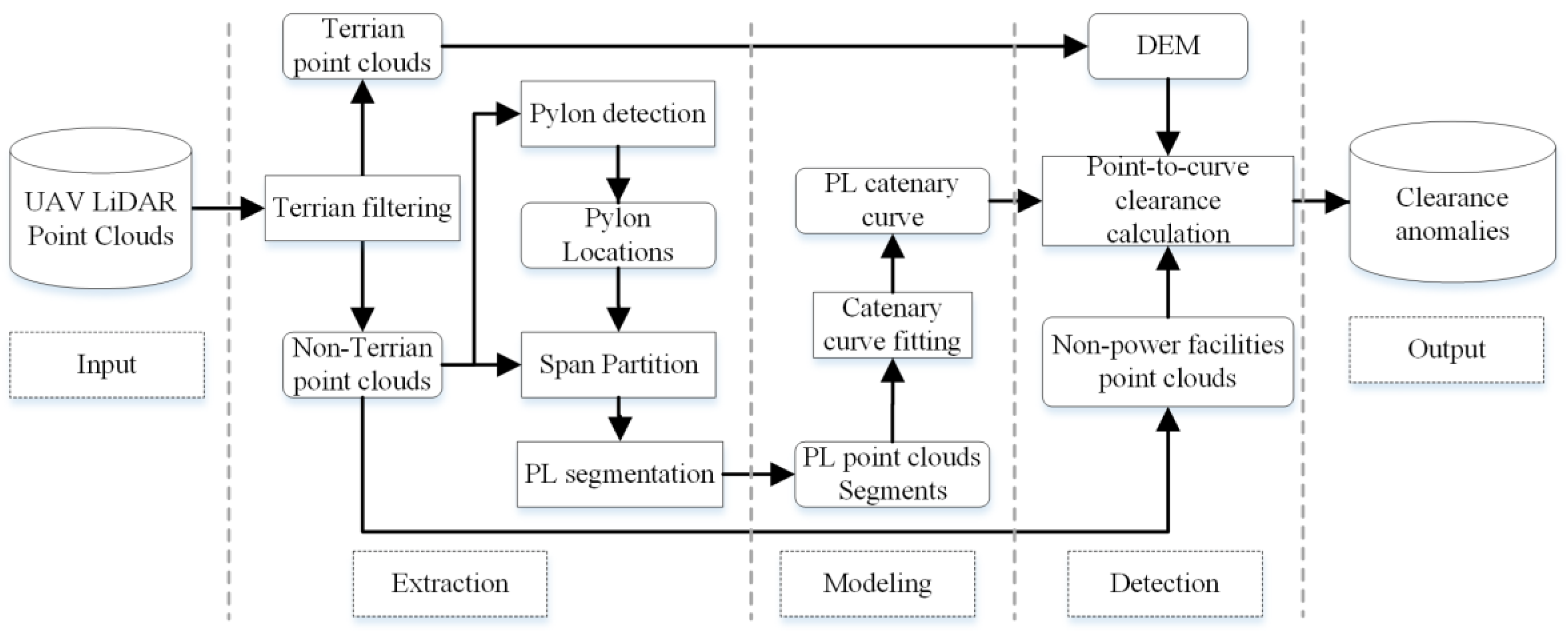
The proposed method comprised three key components, as shown in Figure 1:
- (1)
- Extract the power line point clouds. Partition the point clouds into spans after filtering out the terrain points using two-step adaptive terrain filter and detecting the pylons following a feature map method. The power line point clouds are extracted and further segmented into clusters by combining geometric distribution analysis and conditional Euclidean clustering with linear feature constraints inside the divided spans.
- (2)
- Fit the power line point clouds segments iteratively with 3D catenary curve model using two geometric forms in two 2D dimensions that is represented by a horizontal line and a vertical catenary curve defined by a hyperbolic cosine function to generate continuous mathematical model of the discretely sampled point clouds.
- (3)
- Combine the constructed 3D power line catenary, points of non-power-facility objects and the DEM. The clearance measurements are piecewise solved by nearest search in slices of the non-power-facility objects points/DEM in the span. The locations where the minimum clearance is lower than the safe threshold are considered as clearance anomalies.
2.1. Power Line Point Clouds Extraction
The areas below and within a certain range of the power line are the concern regions of the ROW clearance anomaly detection. Thus, according to the known coarse pylon position and line direction, the UAV collected LiDAR point clouds are trimmed to remove the irrelevant points to acquire the point clouds of the ROW. The isolated noise points (e.g., points on birds) are filtered by eliminating points with less than 10 points in their neighborhoods (2 m radius). The workflow of the power line point clouds extraction is shown in Figure 1 (second column). Firstly, the two-step adaptive terrain filter method [63] is used to filter out the terrain points. Secondly, the pylon point clouds are extracted from the non-terrain point clouds according to the feature map method proposed by Peng et al. [64]. Finally, the ROW point clouds are divided into spans based on the pylon detection results. The power lines point clouds are extracted according to their geometric distribution in local slices of the span point clouds, and are further segmented into clusters by applying conditional Euclidean clustering with linear feature constraints.
The transmission line span refers to the overhead transmission lines area between two pylons, and is the basic component of the power transmission corridors. After the terrain filtering process, the pylon point clouds are iteratively segmented from the raw point clouds according to the density, height difference, and slope feature maps [64]. The precise location and orientation of the pylons are calculated. Then, the ROW point clouds are partitioned into separated spans based on the calculated results. The individual transmission line span is taken as the basic analysis unit for the following power line extraction process.
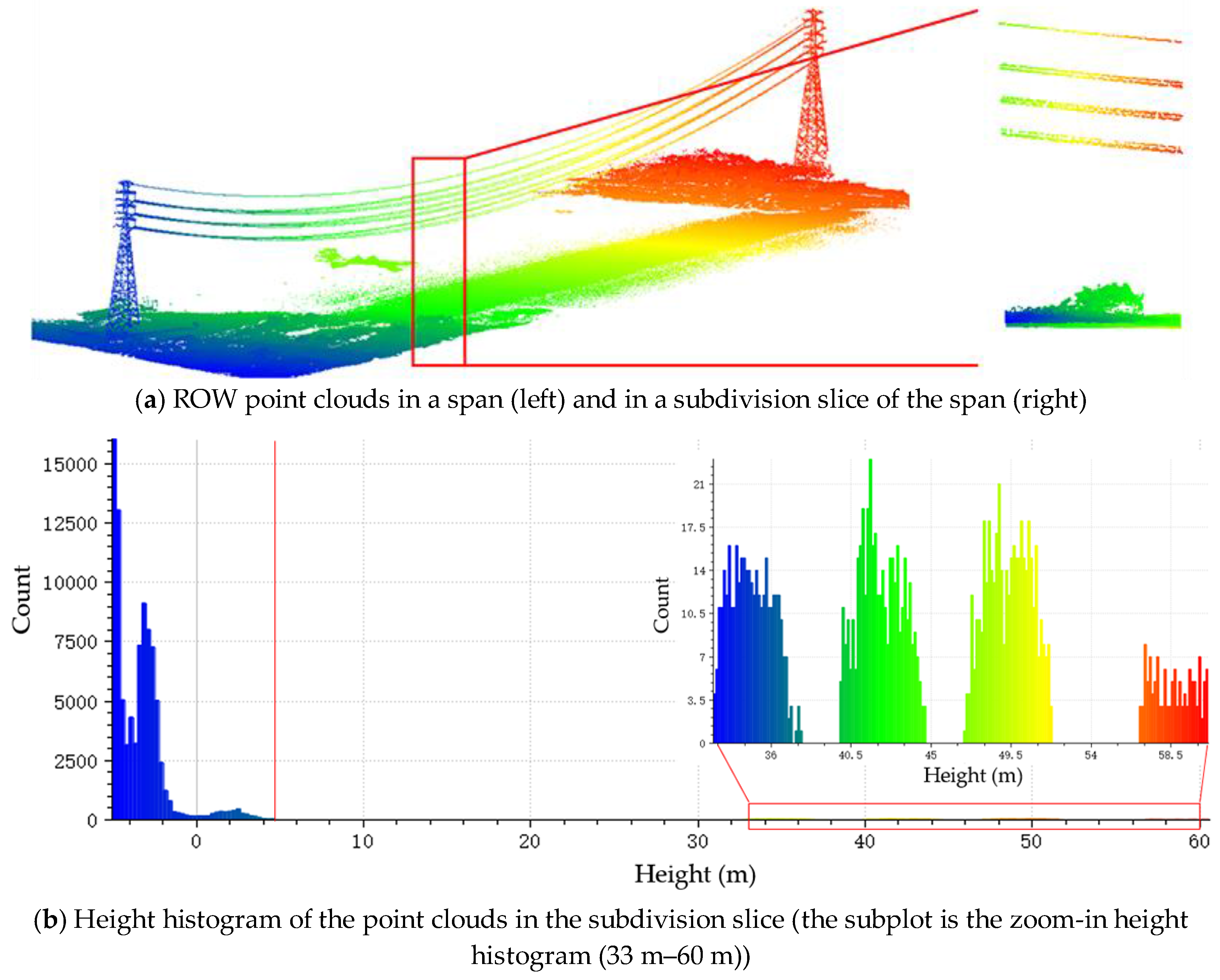
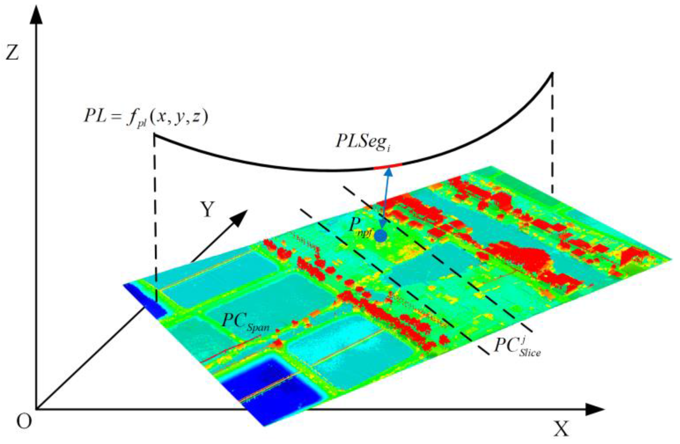
The elevation distribution of the raw points inside the span is usually undulating, especially in the mountainous areas of the HV transmission corridors. The power line and the earth surface cannot be separated by a single classification plane, but an irregular dividing surface. However, the irregular classification surface is hard to solve mathematically. To achieve the classification, a set of classification planes are used in this paper to approximate the irregular surface. Let the point clouds of the transmission line span be . is constructed by a collection of slices of point clouds () divided along the span direction (Figure 2a), as written in Equation (1).
where and are the length of the span and the divided slices of the span ( empirical value: 10 m). is constructed by the point clouds inside the ith slice and is denoted as Equation (2).
is the dividing function that is written as Equation (3).
is the transformation matrix that transforms the direction of the Cartesian coordinate system of the raw point clouds to the parallel direction of the span and its origin to the center point of the span, written as Equation (4).
Let and be the start and end points of the span solved after pylon extraction. The rotation angle is calculated by the direction vector of the span on the XOY plane:
is the translation vector and calculated as . . The terrain fluctuation in a single subdivision slice of the span is relatively small when compared to that of the whole span (Figure 2a). A classification plane (Figure 2b Red line) is estimated to divide the power line points from the other non-terrain points. Height histogram is generated according to the height distribution of the points inside the slice and the peaks are detected. Let be the detected peaks of the height distribution histogram. The two peaks closest to the classification plane are determined as Equation (6).
where is a count function that gives the number of zero value histogram bins in the specified interval. Figure 2a depicts a point cloud slice of the span. The space between the power line points and the non-terrain point is empty, thus the bins correspond to those height spaces that are zero valued (Figure 2b). Equation (6) solves the continuous peak interval with the largest number of zero value bins that contains this empty space. The height of the classification plane () is assigned to the closest zero bin of the low peak bin () in upwards direction, as denoted as Equation (7).
where is the height value of a histogram bin. is a function that produces , if its corresponding histogram bin is zero valued, otherwise the function produces . The classification plane (Figure 2b Red line) divides the points in the slice into two categories. The upper part is taken as the power line points and the lower part is taken as the non-terrain object points.
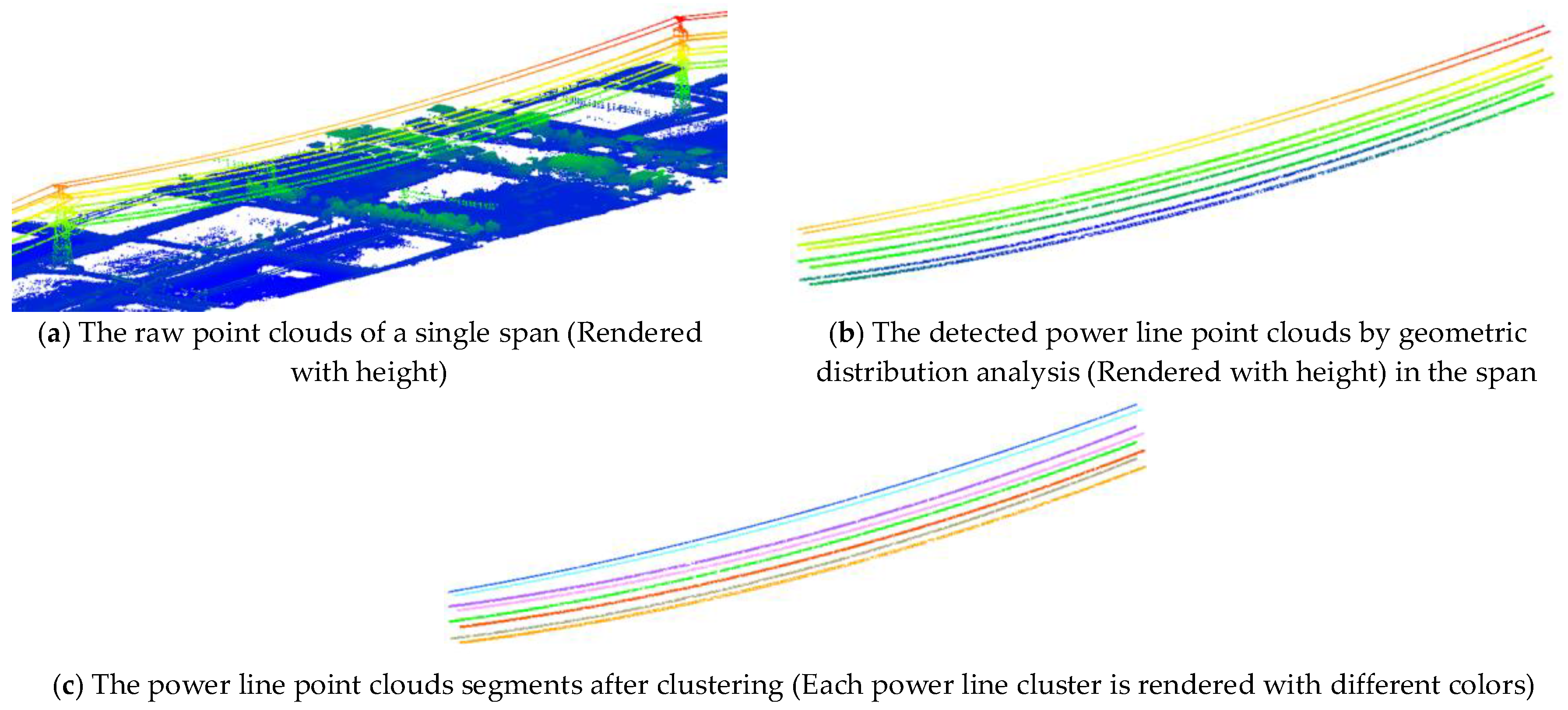
The points of the power line are still not assigned with individual power line label after the dividing process (Figure 3b). To solve this, the conditional Euclidean clustering is adopted with linear feature constraints to segment the classified power line points, resulting in power line points segments for further curve fitting (Figure 3c). Dimensionality feature [65,66] describes the shape of point cloud patch and it has been widely applied in point clouds segmentation and classification [67]. The shape of the power line is a catenary curve with relative low curvature. Segments of the power line curve represents a linear shape that can be measured by dimensionality features. The dimensionality feature of a point on the power line is calculated by its eigenvalue of the local covariance matrix of its neighboring points, defined as Equation (8).
where , are the eigenvalues of the covariance matrix of the neighboring points and are calculated using principal component analysis (PCA). The optimum radius of the neighborhood is determined by adaptive radius computation method that minimizes the entropy function denoted by Equation (9) as proposed by Demantké et al. [66].
The neighborhood radius of each point is increased from to at an incremental rate of . The radius corresponds to the minimal entropy is taken as the optimal neighborhood radius . Once is calculated, the optimal dimensionality feature of a point is calculated according to Equation (8). The neighborhood of the power line points represents a linear structure. In the case of linear point cloud distribution, the principal direction will be the tangent to the curve with , and . With this linear shape constraint and a predefined clustering distance taken as the region growth criteria, the classified power line points are further segmented into power line point segments using Euclidean clustering.
and should be set according to the designed geometry of the inspected HV transmission line. The designed geometry of HV transmission line is available in related power industry standards (e.g., China-GB_50545-2010—code for designing of 110–750 kV overhead transmission line). and in this paper are empirically set to 5 m and 4 m under the circumstance that the inspected HV transmission line is 220 kV. Because the designed minimal distance between the 220 kV conductors is 6 m, they points on different conductors are not grouped into the same cluster or involved in the optimal neighborhood radius search. is empirically set to 1.0 m. is set to 0.2 m according to the point cloud density of the experiment datasets (i.e., 35 points/m2). Smaller is preferred to achieve a better estimate of when the point cloud density is higher, and vice versa. The abovementioned processes are applied to all the spans to extract the power line point segments for further model fitting and clearance measurement.
2.2. Catenary Curve Fitting of the Power Line Point Clouds Segments
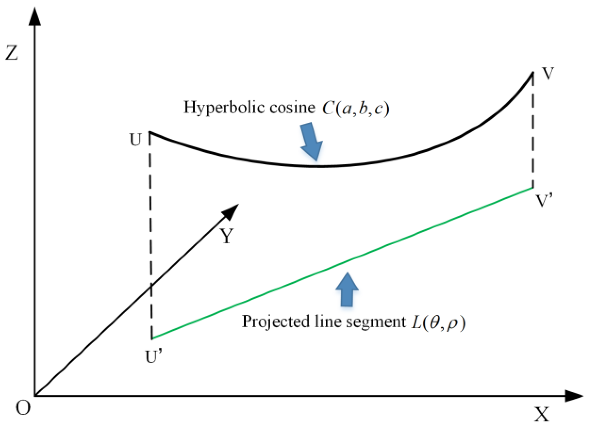
The overhead power line between the pylons is a three-dimensional curve. In ideal condition, it is a homogeneous flexible cable with uniform gravity and equal tension along the line. Currently, there is no standard algorithm for the power line fitting from point clouds because the actual shape of the power line is easily affected by environment changes such as wind, resulting in twisted 3D curves that are difficult to model with a single mathematical model. Existing research showed that the catenary model is ideal and concise for power lines modeling [4,29]. In this paper, the power line is modeled using two geometric forms in two dimensions to construct the 3D catenary curve, as depicted in Figure 4.
The projection of the 3D catenary curve into XOY plane is a line segment. The catenary curve is in the vertical plane (UVU’V’) formed by the projection. The projection of the 3D catenary curve into UVU’V’ plane is modeled as a catenary curve that is defined by a hyperbolic cosine function [27]. Thus, the 3D power line model can be illustrated by a two-dimensional line , in XOY plane and a two-dimensional catenary curve, in UVU’V’ plane, written as Equations (10) and (11).
where X, Y, and Z are coordinates of points in OXYZ reference frame; is the coordinate along the U’V’ axis, in UVU’V’ reference frame which takes the line segment projection as the horizontal axis, UU’ as the vertical axis and U’ as the origin; is the angle between the normal vector of the line segment and the X-axis; is the distance between the line segment and the origin; and (a,b) are parameters for the origin translation. The ratio between the tension and the weight of the hanging flexible wire is denoted by scalar factor c. Let the points in the ith clustered power line segment be . The 2D principal directions in XOY plane of are solved by PCA. The is calculated as the angle between the normal vector of and the X-axis. The is then solved as , according to Equation (10). The ith catenary curve in plane is solved by minimizing the difference between the observed Z value and the fitted Z value of all the points in the ith segment , that is written as Equation (12).
where is the transformation matrix that transforms the coordinate in OXYZ reference frame to in UVU’V’ reference frame. The study by Ceres [68] is used to solve Equation (12). To merge point segments that belong to the same curve, we iteratively add point segments to current fitted curve to find all the point segments belonging to the same power line. Once the of are fitted, points in each of the rest segments (denote as ) in the span are added to to fit a new catenary curve. If the per-point fit error (Equation (12)) is not greater than predefined threshold (empirical value 0.2 m). The added point segments are taken as inliers of the currently fitted power line curve and removed from the need-to-fit point segments set. Otherwise, the added point segments are taken as outliers which means the added points do not belong to the current fitted catenary curve. Above mentioned processes are repeated until all the power line point cloud segments in the span are assigned to catenary curves.
2.3. Clearance Calculation and Anomaly Detection
In essence, the clearance anomaly detection calculates the distance between the fitted 3D power line curves and the non-power-facility objects beneath it in the transmission line corridor to detect the spots where the safe clearance threshold is exceeded. It is complex and inefficient to calculate analytical solution of the distance from a given point to a specific 3D curve [69,70]. To simplify the distance measurements of the points on non-terrain objects to power line catenary curves, we propose a piecewise clearance calculation method based on differential geometry.
The continuous power line catenary curve in its span is sampled into ordered curve segments with unified sampling distance . The distance between the points of non-power-facility objects and (Figure 5) is denoted as Equation (13).
where is the distance calculation function. and are the start and end x coordinate of the . If is small enough, the length of the curve segments decreases and can be approximated by a set of scatter points along the curve, written as . Thus, the point-to-curve distance calculation degenerates to point-to-point distance measurement, as denoted by Equation (14).
Two types of data are used for calculating the distance: the classified non-power-facility objects point clouds (vegetation in our scope) and DEM in the case there are missing point cloud data due to water surface, etc. (Figure 6). To balance the accuracy and the efficiency of the distance calculation in Equation (14), is set to 0.05 m empirically. The point clouds in the span are divided into n slices according to Equations (1)–(5). The individual is used to construct n k-d tree structures together with the . For the ith point on the , , the are calculated following Equations (10) and (11). The distance between the and the DEM in vertical direction is calculated and denoted as -to-DEM distance. The closest point cloud slice of the is found by its projection on XOY plane. Furthermore, the jth (closest slice) k-d tree structure is used to efficiently find the closest point to in point clouds of non-power-facility objects in , result in the clearance measurement. While the jth k-d tree structure does not return a validate point or the calculated distance is bigger than the -to-DEM distance, -to-DEM distance is taken as the clearance measurement.
There are multiple kinds of targets included in the ROW point clouds collected by UAV. As the HV transmission lines are usually located in rural or depopulated areas, the non-power-facility objects in the line corridors consist of major natural vegetation and seldom artificial objects such as buildings or other power lines crossing the transmission line corridor. The safe clearance thresholds are related to the category of the non-power-facility objects. The calculated distances are compared with clearance threshold defined in related regulations. If the minimum distance is greater than the safe distance threshold, it is considered safe, otherwise, it is a clearance anomaly.
3. Experiments and Analysis
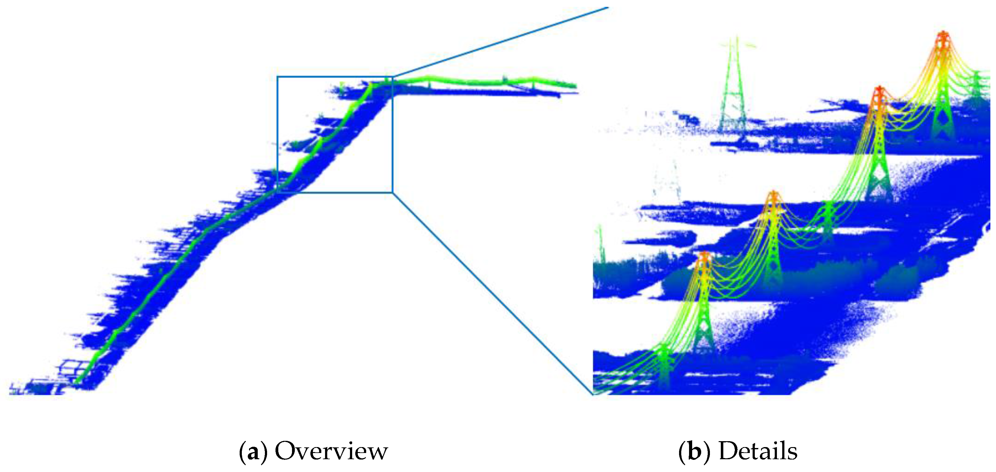
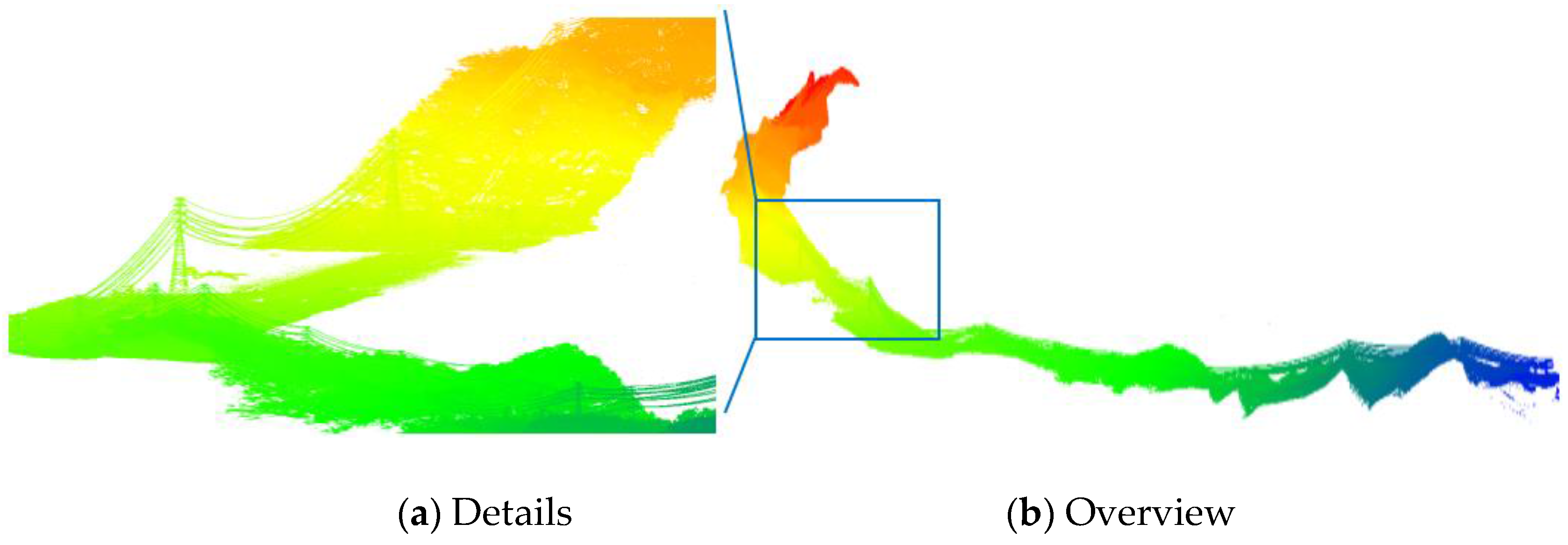
Experiments were performed to validate the effectiveness and accuracy of the proposed diagnostic algorithm for the clearance anomaly detection using two point cloud datasets captured by a large UAV-borne power line inspection robot [18] (Figure 7) equipped with a custom built LiDAR system. The sensor specifications of the equipped LiDAR are listed in Table 1. The post-processed accuracy specifications of the custom built POS are listed in Table 2. Considering the terrain diversity of the ROW, two 220 kV transmission line located in Guangdong Province, China are chosen as the inspection targets with the help of the local power supply bureau. The operation altitude/navigation speed of the UAV are set to 150 m (above the ground) and 7 m/s, respectively. The laser pulse rate of the scanner is set to 300 kHz. The acquisition procedures concerning the autonomous navigations of the UAV, etc. are elaborated by Peng et al. [18,71]. The description of the datasets is shown in Table 3. The ROW 1 is featured with relatively flat terrain in which large areas of farmland areas exists. The length of the ROW 1 inspection section is 9.2 km with a total of 21 pylons. The terrain is mainly plain paddy fields, with about 2 km of cross-river topography and 3 km of gentle hills. ROW 1 dataset includes 99.31 million points and its point cloud density is 35 points per square meter. The terrain of ROW 2 is mountainous and covered with vegetation. ROW 2 inspection section is 6.2 km with a total of 16 pylons. The terrain is an undulating chain of hills. The point cloud density of ROW 2 dataset is 34.3 points per square meter and the total number of points is 53.2 million. The raw LiDAR point cloud data and the local enlarged snapshot of ROWs 1 and 2 are shown in Figure 8 and Figure 9. Because the inspected area is located in a non-residential region, there are no buildings inside the ROWs. Experiment data for ROWs 1 and 2 are collected on calm weather day. The datasets express no wind-bias phenomenon.
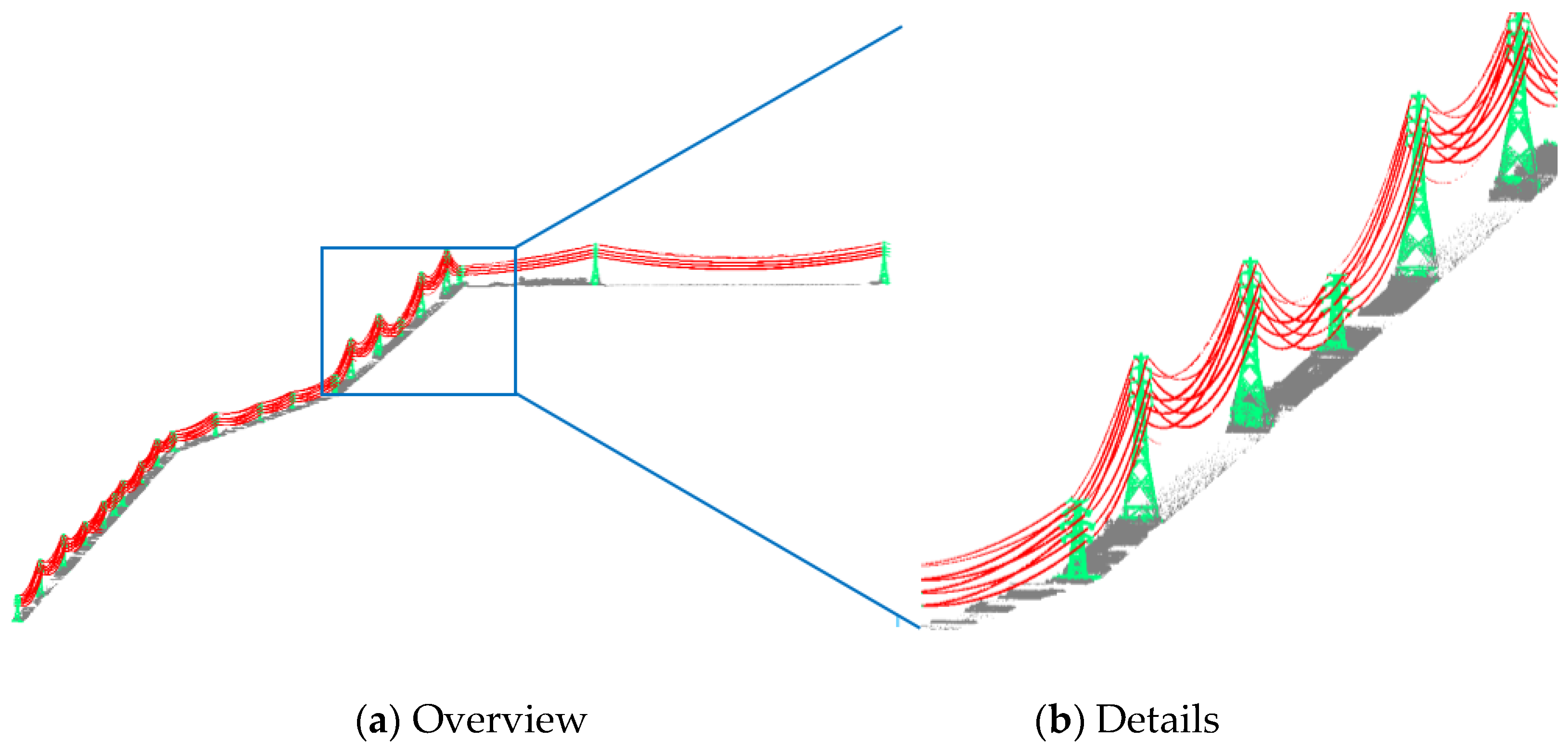
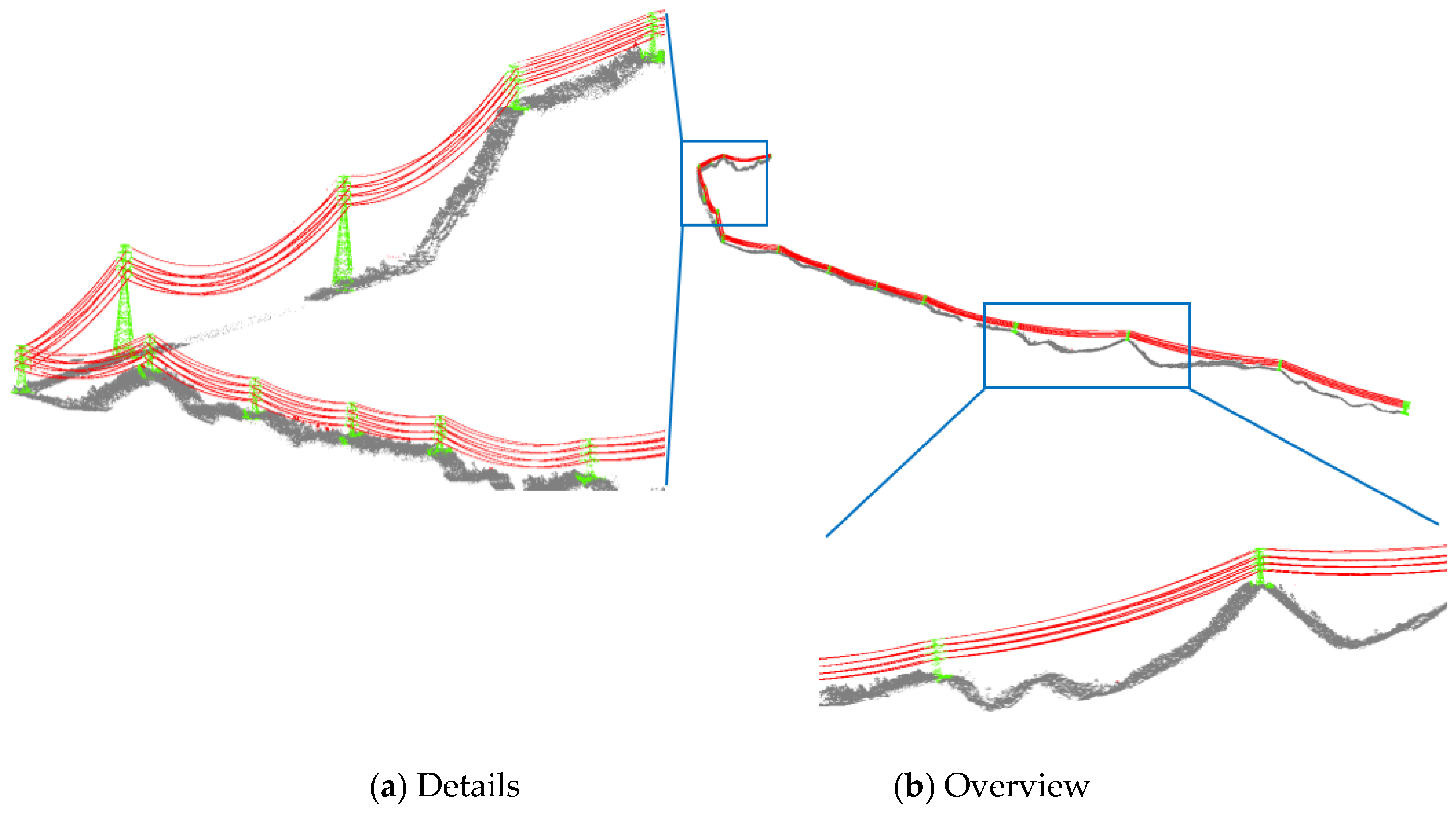
According to the known coarse position and direction of the PL, the LiDAR point cloud collected by our UAV inspection robot is trimmed to obtain concerned point clouds inside the ROW which represent a regular strip pattern. The power line point clouds are extracted and fitted with the proposed method described in Section 2.1 and Section 2.2. Figure 10 and Figure 11 shows the power line extraction results of ROW 1 and 2 datasets, respectively. The extracted power lines, pylons, and the non-power-facility objects (i.e., vegetation in our scope) are rendered in red, green and gray, respectively. There are 160 and 120 conductors and 21 and 16 pylons detected in ROW 1 and ROW 2 datasets, respectively, which is in accordance with the real scene. The power line point clouds are extracted according to their geometric distribution in local span point clouds slices for further clustering (Section 2.1). The slice length is set to 10 m. The should be determined based on the slope characteristic of the ROWs. Small (e.g., 10 m) is preferred for datasets with large slope values because more classification planes will be generated to approximate the irregular dividing surface, resulting in complex terrain adaptability. For flat terrains, could be set to a large value (e.g., 30 m) to accelerate the power line point cloud segmentation process. Despite the efficiency requirement, is recommended to be set to a small value (5 m–15 m) to guarantee a high quality point clouds classification results.
To quantify the performance of the power line point clouds extraction method, the ground truth of the power line point clouds are labeled manually and compared with the automatic detection results. The precision, recall, and F-measure of the power line points are used to evaluate the results:
where TP is true positive, FP is false positive, and FN is false negative, which denote the number of points that are labeled as power line correctly and incorrectly, and falsely labeled as other category, respectively. F is the harmonic mean of the recall and precision. The positional accuracy of the catenary curve fitting described in Section 2.2 is evaluated by measuring the max (PMAX) and root-mean-square error (PRMSE) fitting error. Table 4 shows the overall performance of proposed approach in terms of the abovementioned five criteria for power line extraction and fitting.
In regard to the accuracy of the power line point clouds extraction: (1) the FP points are mainly the points on the insulators and the linear shaped connection hardware that are incorrectly labelled as power line points; and (2) the FN points are the points that are excluded when the linear shape constrained Euclidean clustering are performed. This region growth clustering process may reject some of the true power line points if the dimensionality feature is not linear shaped or the point spaces are larger than the clustering distance threshold. The overall F-Measure is 0.956 on average. The mislabeled power line points are majorly located at the ends of the conductor where are considered less crucial to the clearance anomaly detection. Because the end points of the power line are usually much higher than the sag points. The performance is considered to be better than the power line point clouds extraction algorithm proposed by Kim et al. [45,53] and close to the algorithm proposed by Guan [29] using very dense vehicle-borne LiDAR data, in terms of precision, recall, and F-measure. The average model fitting error PMAX and PRMSE are 0.153 m and 0.078 m, respectively. The model fitting accuracy is related to the mathematical model of the catenary curve mentioned in Section 2.3, the point density and many other factors such as the accuracy of the laser point clouds or windy weather. The achieved PMAX and PRMSE are considered to be fair for clearance anomaly detection application utilizing the experiment datasets.
The clearance between the conductor and non-power-facility objects in the ROW is calculated and the locations exceeding the safe threshold is found, according to the clearance anomaly detection method proposed in Section 2.3. The safe clearance threshold is chosen following the relevant regulation that is the power industry standard of China DL/T 741-2010—“Operation code for overhead transmission line”. Eleven clearance anomalies have been discovered after the detection process, as listed in Table 5. There are two and nine clearance anomalies detected in ROW 1 and ROW 2 datasets, respectively. Ten out of the eleven clearance anomalies (threshold: 4.5 m) are confirmed to be high vegetation through visual inspection. The second clearance anomaly of ROW 1 (threshold: 4 m) is a low voltage transmission line (380 V) crossing the HV 200 kv transmission line corridor.
To quantitatively analyze the clearance anomalies detection results derived from the proposed method, the calculated values are compared with the results derived from manual surveying and another clearance measuring algorithm proposed by Peng et al. [31] (Denoted by Peng’s algorithm). The distances between the power line and the non-power-facility objects in the two ROWs are manually measured in the point clouds and taken as the ground truth of the clearance measurements at the locations where the safe thresholds are exceeded. The comparison results are shown in Table 5 and Table 6. The minimum and maximum error between the clearance obtained from the proposed detection algorithm and the manually measured true value is 0.02 m and 0.14 m, respectively. The average error and the root mean square error is 0.08 m and 0.04 m. The minimum error and maximum error of Peng’s algorithm [31] is 0.04 m and 0.31 m, the average error is 0.17 m, and the root mean square error is 0.09 m. It can be learned from the statistics of the comparison results that the algorithm proposed in this paper outperforms Peng’s algorithm [31], and the difference between the clearance measurements algorithm delivered and the manual surveyed references are within decimeter (average error is 0.08 m). Compared with Peng’s algorithm [31], the improvement of the proposed algorithm achieved in this paper is mainly attributable to the different extraction and fitting method of the power line. The proposed method improves the accuracy of clearance measuring by geometric distribution analysis in local span point clouds slices and replacing segmented centroid fitting in Peng’s algorithm [31] with catenary fitting, thus obtaining more accurate results.
4. Discussion
The experiment results mentioned above have proven the effectiveness and accuracy of the proposed clearance anomaly detection algorithms utilizing UAV-borne LiDAR data. The detected results illustrate that the proposed method can extract anomalies exceeding the minimal clearance thresholds, such as tree encroachments. The differences between the clearance measurements delivered by the proposed algorithm and the manual surveyed references in the point clouds are within decimeter. The UAVs are more wind-sensitive than the manned helicopters or fixed wing planes. To guarantee a safe inspection, the experiment datasets are collected in calm weather condition. The datasets express no wind-bias phenomenon. Windy weather will affect the catenary shape of the conductors, resulting in precision losses of the catenary fitting. Under this circumstance, a wind adaptive power line modeling strategy such as minimum description length approach [14] should be used to fit the power line point clouds segments.
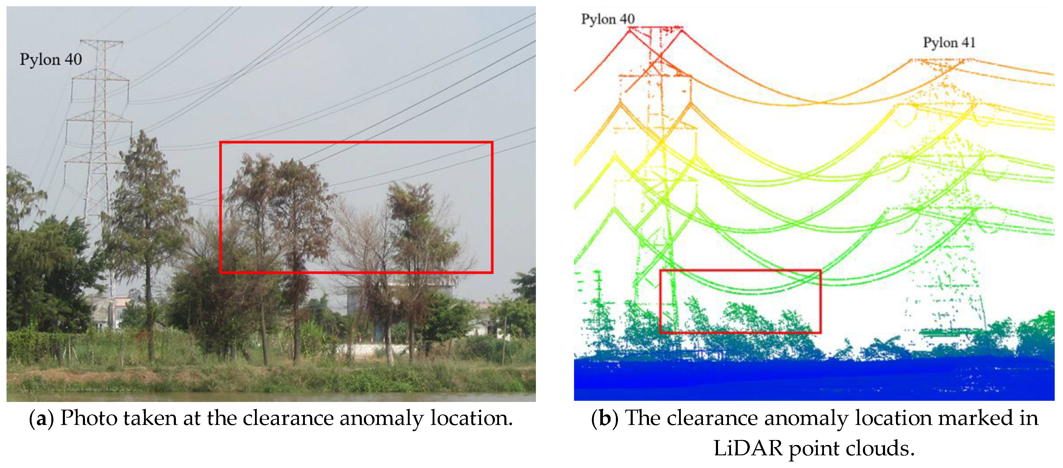
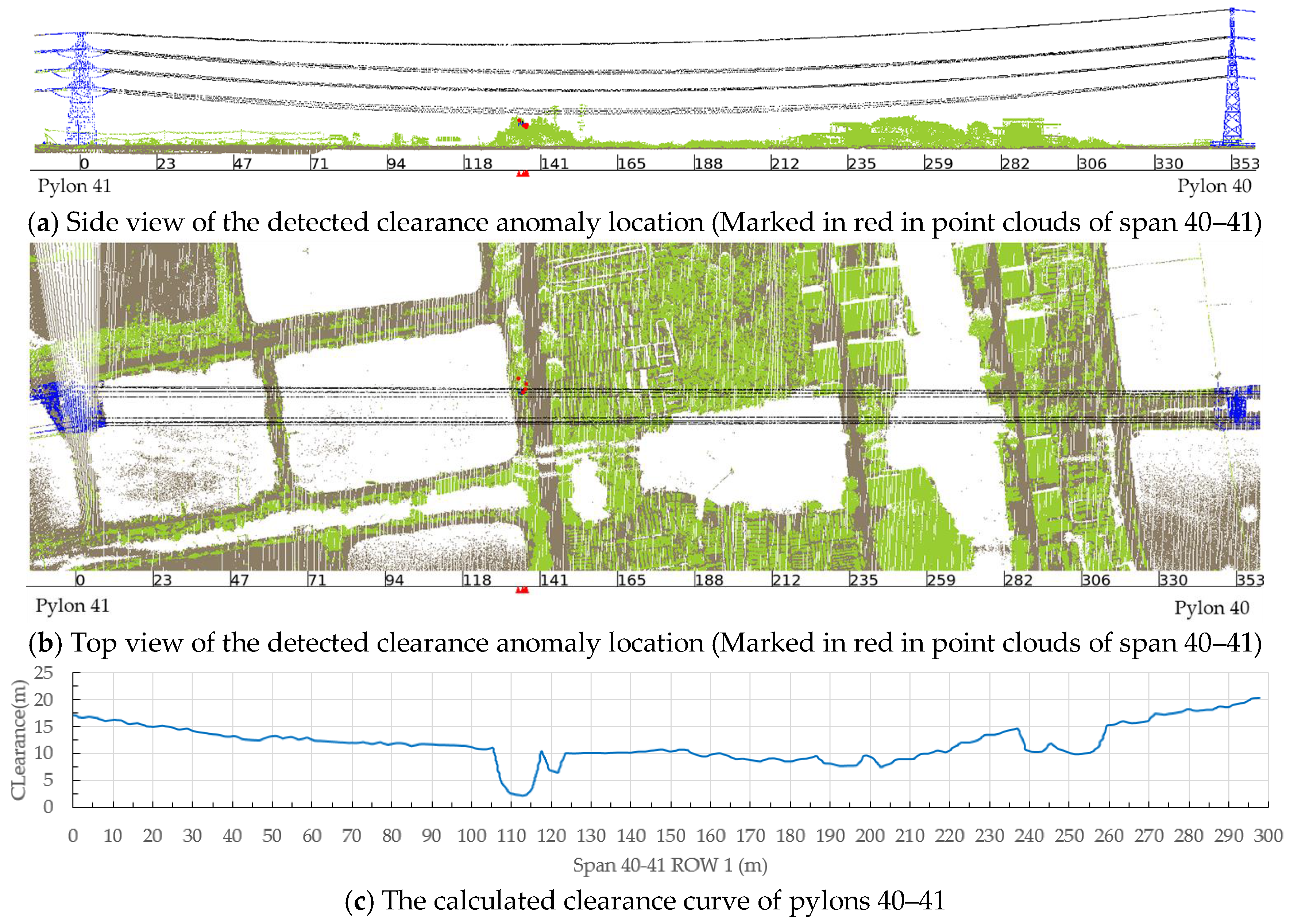
The point density is vitally important in the automatic clearance anomaly detection process. The lack of laser point clouds density will lead to less well sampled point clouds on the non-power-facility objects in the ROW, resulting in loss of precision of the clearance measurement. To investigate the impact of the point clouds density on the clearance calculation, we compared the results derived from the proposed algorithm and the field survey. An easy-to-reach detected clearance anomaly location (Figure 12) was selected for field verification of the clearance anomaly detection results short after the data collection, restricted by the inconvenient transportation caused by the complex terrain of the experimental regions. The surveyed clearance fault locates on the C phase (lowest conductor) of the power lines between pylons 40 and 41 in the ROW 1 dataset. The distance between the power line and the tree encroachment is manually measured by a total station. The clearance anomaly location is shown in the photo taken in the field during the verification process (Figure 12a) and in the LiDAR point clouds (Figure 12b), respectively. The staff of the local power supply bureau uses total station to measure the distance between low point on the C phase of the power lines and the underlying tree canopy, and the result is reported as 2.42 m. The clearance calculated by the proposed algorithm is 2.22 m, resulting in a 0.20 m difference. At this clearance anomaly location, the manual measurement of the clearance in the laser point clouds is 2.31 m that is 0.09 m different from that of the proposed algorithm. The detected clearance anomaly are depicted in Figure 13a,b. The corresponding clearance curve of the span 40–41 is shown in Figure 13c.
In the field verification working condition, many error sources can cause the observed 0.20 m error, including the manual alignment error between the treetop and the low point on the conductor when operating the total station, the deviation caused by wind influencing the actual treetop position, etc. It is worth noting that insufficient LiDAR point cloud density may cause the precision related issues observed. In our experiment, the point density is about 35 points/m2. The lack of point density should be considered as one of the reasons for the measurement deviation. The laser point clouds fail to reconstruct the full geometry of the top of the tree encroachment because of the relatively low point density, which directly leads to the measurement deviation.
Existing studies related to tree height measurements usually took advantage of the low flying altitude of the UAV and repeated scans to achieve a very high point density to guarantee accurate results in the investigated forest plots. Jaakkola et al. [59] built the first UAV LiDAR system for tree measurements. The density of its generated point clouds of the test flights was 100–1500 points/m2. Wallace el al. [60,61] presented estimates of tree location (mean deviation (MD) of less than 0.48 m) and tree height (MD of 0.35 m) achieved using point clouds of up to 300 points/m2 density collected by their customized UAV LiDAR. Recently, UAV laser scanning-based automated tree-level field reference collection has been proven feasible using point clouds with an average density of 800 points/m2 [62]. In addition, the UAV LiDAR system (e.g., RiCOPTER) has the potential to perform comparable to terrestrial laser scanning for estimating forest canopy height utilizing its very high density point clouds (3000–5000 points/m2) [54]. However, those studies mainly focus on the refined investigation of forest plots within relatively small areas (e.g., 500 m2) using low altitude (e.g., 50 m above the ground) UAV LiDAR data.
The ROW inspection applications are different from forest applications. The inspected ROWs are usually long (>5 km) during each flight. Very low flying altitude and repeated scans is considered as inefficient and dangerous (threats to the power facilities). It is not technically sound and applicable to endeavor to collect very high density point clouds (e.g., >1000 points/m2) for detailed tree top modeling in ROW inspection applications. Finding an appropriate point density for ROW inspection is a compromise and balance of the efficiency and the precision. The 35 points/m2 point density of the developed UAV LiDAR system is already much higher than the general point density of the standard manned air-borne LiDAR system (e.g., typical value: 10 points/m2). Compared with the manual measurements in the point clouds, the proposed algorithm achieved an average error of 0.08 m and RMSE of 0.04 m (Table 5 and Table 6), which is considered applicable according to the power industry standard of China DL/T 741-2010—“Operation code for overhead transmission line”. The proposed clearance anomaly detection method only considers the current status of the ROW. Thus, in future work, the dynamic feature of the conductors and the objects in the ROW should be considered. Geometric ecological modeling of individual trees will be carried out to simulate the dynamic change of the forest geometrical shape under different environment conditions to find the potential clearance faults. Environmental adaptive power line modeling methods will be explored to model the changes of the conductors under different weather conditions for better detection of the clearance anomalies.
5. Conclusions
ROW clearance anomaly detection measures the distance between the power lines and the surrounding non-power-facility objects in the corridor such as trees to find the anomalies exceeding the safe distance thresholds defined in the regulations. It is one of the important work contents of the power grid operation and maintenance. In this study, an automatic clearance anomaly detection method utilizing LiDAR point clouds collected by a large-scale UAV power line inspection system was proposed, which employed a novel power line point cloud extraction algorithm combining geometric distributions analysis in span slices and clustering with linear feature constraints in span for further differential geometry based piecewise point-to-catenary clearance calculation. Multiple LiDAR point clouds datasets collected at two 220 KV transmission line corridors featuring different terrain characteristic (flat terrain, gentle and undulating steep hills) by our rotor-wing large-UAV power inspection robot were used to validate the robustness against different terrain, effectiveness and precision of the proposed method in this paper. Qualitative and quantitative analysis of the detection results were made by comparing with manual measurements in the LiDAR point clouds, another algorithm [31] in the same category and on-site field survey. The experimental results show that the proposed method outperforms the algorithm proposed by Peng et al. [31], and can effectively detect the clearance anomalies with a decimeter accuracy using our UAV power line inspection robot in both flat and steep terrain. The overall F-Measure of the power line point clouds extraction is 0.956 on average. The PMAX and PRMSE model fitting error of the conductors are 0.153 m and 0.078 m, respectively. The average error and the RMSE of the final clearance measurement is 0.08 m and 0.04 m. The operation altitude/navigation speed of the UAV are set to 150 m (above the ground) and 7 m/s, respectively. The laser pulse rate of the scanner is set to 300 kHz. The point density of the generated point cloud is about 35 points/m2 in the inspected ROW1-2 environments. The achieved point density (35 points/m2) is higher than the general point density of the standard manned air-borne LiDAR system (e.g., typical value: 10 points/m2). Insufficient LiDAR point cloud density may cause precision losses in the clearance measurement. Choosing an appropriate point density objective before flight for ROW inspection is a compromise and balance of efficiency and precision. The clearance detection method proposed is decimeter-accurate using the LiDAR data collected by our UAV inspection robot with abovementioned operation specifications. Lower flying altitude, higher laser pulse rater and repeated scans are suggested to increase the point density of the acquired point clouds, thus to further improve the accuracy of the clearance measurements. The performance of the proposed clearance anomaly detection method and the UAV LiDAR ROW inspection system meets the requirements of current ROW inspection standard of the power industry in China. According to the preliminary research presented, inspection with UAV LiDAR system has shown great potentials in improving the efficiency, precision, flexibility and the degree of automation of the ROW clearance anomaly detection in the power line risk management. The UAVs are wind-sensitive. Also, windy weather will affect the catenary shape of the conductors, resulting in wind-bias phenomenon that leads to precision losses of the catenary fitting. The windy weather adaptability is the main limitation of our UAV inspection robot and the proposed automatic clearance anomaly detection method. In our future research work, individual trees and conductors will be modeled with dynamic ecological and geometrical models to simulate their dynamic changes under different environment conditions, thus to find the existing and potential clearance faults in all weather conditions.
Acknowledgments
The work presented in this article was substantially supported by National Natural Science Foundation Project of China (No. 41701530 and 41531177), The National Science Fund for Distinguished Young Scholars of China (No. 41725005), China Postdoctoral Science Found (No. 2016M600614), China Southern Power Grid Corporation Science and Technology Project (No. GD-KJXM201509), and LIESMARS Special Research Funding and Key Laboratory of Spatial Data Mining & Information Sharing of Ministry of Education, Fuzhou University (No. 2018LSDMIS06).
Author Contributions
Chi Chen designed and implemented the proposed method and the experiments, analyze the experiments results, wrote and revised the paper. Bisheng Yang contributed to the analysis of the experiments results, revising the methodology and the paper. Shuang Song contributed to the discussion, coding, analysis of the experiments results and revision of the paper. Xiangyang Peng contributed to solve the power transmission related issues, chose the experiment location and setups and helped with the field verification. Ronggang Huang helped with the discussion and revision of the paper.
Conflicts of Interest
The authors declare no conflict of interest.
References
- Strmiska, R.G. Five Important Power Line Component anomalies. In Thermosense XXII, Orlando, FL, 24–28 April 2000; International Society for Optics and Photonics: Bellingham, WA, USA, 2000; pp. 85–91. [Google Scholar]
- Neal, M. Aerial laser surveying: Data enables Arizona public service to locate and eliminate clearance violations and facilitate long-range planning. Transm. Distrib. World 2009, 61, 5–9. [Google Scholar]
- Mirallès, F.; Pouliot, N.; Montambault, S. State-of-the-art review of computer vision for the management of power transmission lines. In Proceedings of the 2014 3rd International Conference on Applied Robotics for the Power Industry (CARPI), Foz do Iguassu, Brazil, 14–16 October 2014; IEEE: Piscataway, NJ, USA, 2014; pp. 1–6. [Google Scholar]
- Jwa, Y.; Sohn, G. A piecewise catenary curve model growing for 3D power line reconstruction. Photogramm. Eng. Remote Sens. 2015, 78, 1227–1240. [Google Scholar] [CrossRef]
- Matikainen, L.; Lehtomäki, M.; Ahokas, E.; Hyyppä, J.; Karjalainen, M.; Jaakkola, A.; Kukko, A.; Heinonen, T. Remote sensing methods for power line corridor surveys. ISPRS J. Photogramm. Remote Sens. 2016, 119, 10–31. [Google Scholar] [CrossRef]
- Aggarwal, R.; Johns, A.; Jayasinghe, J.; Su, W. An overview of the condition monitoring of overhead lines. Electr. Power Syst. Res. 2000, 53, 15–22. [Google Scholar] [CrossRef]
- Katrasnik, J.; Pernus, F.; Likar, B. A survey of mobile robots for distribution power line inspection. IEEE Trans. Power Deliv. 2010, 25, 485–493. [Google Scholar] [CrossRef]
- Wanik, D.W.; Parent, J.R.; Anagnostou, E.N.; Hartman, B.M. Using vegetation management and lidar-derived tree height data to improve outage predictions for electric utilities. Electr. Power Syst. Res. 2017, 146, 236–245. [Google Scholar] [CrossRef]
- Sohn, G.; Ituen, I. The way forward: Advances in maintaining right-of-way of transmission lines. Geomatica 2010, 64, 451–462. [Google Scholar]
- Wolf, G. Lidar: Illuminating hazardous vegetation. Transm. Distrib. World 2010, 62, 13–18. [Google Scholar]
- Mills, S.J.; Castro, M.P.G.; Li, Z.; Cai, J.; Hayward, R.; Mejias, L.; Walker, R.A. Evaluation of aerial remote sensing techniques for vegetation management in power-line corridors. IEEE Tran. Geosci. Remote Sens. 2010, 48, 3379–3390. [Google Scholar] [CrossRef] [Green Version]
- Ahmad, J.; Malik, A.S.; Xia, L. Vegetation monitoring for high-voltage transmission line corridors using satellite stereo images. In Proceedings of the 2011 National Postgraduate Conference (NPC), Kuala Lumpur, Malaysia, 19–20 September 2011; IEEE: Piscataway, NJ, USA, 2011; pp. 1–5. [Google Scholar]
- Ahmad, J.; Malik, A.S.; Xia, L.; Ashikin, N. Vegetation encroachment monitoring for transmission lines right-of-ways: A survey. Electr. Power Syst. Res. 2013, 95, 339–352. [Google Scholar] [CrossRef]
- Jaw, Y.; Sohn, G. Wind adaptive modeling of transmission lines using minimum description length. ISPRS J. Photogramm. Remote Sens. 2017, 125, 193–206. [Google Scholar] [CrossRef]
- Springer, G. Trimming Your Way to a More Reliable Future. Transm. Distrib. World 2010, 62, 38–41. [Google Scholar]
- Ahmad, J.; Malik, A.S.; Abdullah, M.F.; Kamel, N.; Xia, L. A novel method for vegetation encroachment monitoring of transmission lines using a single 2D camera. Pattern Anal. Appl. 2015, 18, 419–440. [Google Scholar] [CrossRef]
- Liu, H.; Chen, W.; Gao, X.-H. Analysis of vegetation-related failures on transmission lines from the viewpoint of blackouts. Power Syst. Technol. 2007, 31, 67–69. [Google Scholar]
- Peng, X.; Chen, C.; Rao, Z.; Yang, B.; Mai, X.; Wang, K. Safety inspection and intelligent diagnosis of transmission line based on unmanned helicopter of multi sensor data acquisition. High Volt. Eng. 2015, 41, 159–166. [Google Scholar]
- Zhang, J.; Huang, G.; Liu, J. SAR remote sensing monitoring of the Yushu earthquake disaster situation and the information service system. J. Remote Sens. 2010, 14, 1038–1052. [Google Scholar]
- Eriksson, L.E.; Fransson, J.E.; Soja, M.J.; Santoro, M. Backscatter signatures of wind-thrown forest in satellite SAR images. In Proceedings of the 2012 IEEE International Geoscience and Remote Sensing Symposium (IGARSS), Munich, Germany, 22–27 July 2012; IEEE: Piscataway, NJ, USA, 2012; pp. 6435–6438. [Google Scholar]
- Kobayashi, Y.; Karady, G.G.; Heydt, G.T.; Olsen, R.G. The utilization of satellite images to identify trees endangering transmission lines. IEEE Trans. Power Deliv. 2009, 24, 1703–1709. [Google Scholar] [CrossRef]
- Sun, C.; Jones, R.; Talbot, H.; Wu, X.; Cheong, K.; Beare, R.; Buckley, M.; Berman, M. Measuring the distance of vegetation from powerlines using stereo vision. ISPRS J. Photogramm. Remote Sens. 2006, 60, 269–283. [Google Scholar] [CrossRef]
- Stockton, G.R.; Tache, A. Advances in applications for aerial infrared thermography. Proc. SPIE 2006, 6205. [Google Scholar] [CrossRef]
- Wronkowicz, A. Automatic fusion of visible and infrared images taken from different perspectives for diagnostics of power lines. Quant. InfraRed Thermogr. J. 2016, 13, 155–169. [Google Scholar] [CrossRef]
- Guo, B.; Li, Q.; Huang, X.; Wang, C. An improved method for power-line reconstruction from point cloud data. Remote Sens. 2016, 8, 36. [Google Scholar] [CrossRef]
- Zhu, L.; Hyyppä, J. Fully-automated power line extraction from airborne laser scanning point clouds in forest areas. Remote Sens. 2014, 6, 11267–11282. [Google Scholar] [CrossRef]
- McLaughlin, R.A. Extracting transmission lines from airborne LIDAR data. IEEE Geosci. Remote Sens. Lett. 2006, 3, 222–226. [Google Scholar] [CrossRef]
- Chen, C.; Mai, X.; Song, S.; Peng, X.; Xu, W.; Wang, K. Automatic power lines extraction method from airborne LiDAR point cloud. Geomat. Inf. Sci. Wuhan Univ. 2015, 40, 1600–1605. [Google Scholar]
- Guan, H.; Yu, Y.; Li, J.; Ji, Z.; Zhang, Q. Extraction of power-transmission lines from vehicle-borne lidar data. Int. J. Remote Sens. 2016, 37, 229–247. [Google Scholar] [CrossRef]
- Ax, M.; Thamke, S.; Kuhnert, L.; Kuhnert, K.D. UAV based laser measurement for vegetation control at high-voltage transmission lines. Adv. Mater. Res. 2013, 614–615, 1147–1152. [Google Scholar] [CrossRef]
- Peng, X.; Chen, C.; Xu, X.; Xu, W. Transmission lines corridor safety distance diagnosis based on airborne laser scanning point cloud. Power Syst. Technol. 2014, 38, 3254–3259. [Google Scholar]
- Tong, W.-G.; Li, B.-S.; Yuan, J.-S.; Zhao, S.-T. Transmission line extraction and recognition from natural complex background. In Proceedings of the 2009 International Conference on Machine Learning and Cybernetics, Hebei, China, 12–15 July 2009; IEEE: Piscataway, NJ, USA, 2009; pp. 2473–2477. [Google Scholar]
- Wu, Q.; An, J. Extraction of power lines from aerial images based on Hough transform. Proc. SPIE Int. Soc. Opt. Eng. 2010, 7862. [Google Scholar] [CrossRef]
- Zhang, X.; An, J.; Chen, F. A method of insulator fault detection from airborne images. In Proceedings of the 2010 Second WRI Global Congress on Intelligent Systems (GCIS), Wuhan, China, 16–17 December 2010; IEEE: Piscataway, NJ, USA, 2010; pp. 200–203. [Google Scholar]
- Yan, G.; Li, C.; Zhou, G.; Zhang, W.; Li, X. Automatic extraction of power lines from aerial images. IEEE Geosci. Remote Sens. Lett. 2007, 4, 387–391. [Google Scholar] [CrossRef]
- Yang, T.W.; Yin, H.; Ruan, Q.Q.; Da Han, J.; Qi, J.T.; Yong, Q.; Wang, Z.T.; Sun, Z.Q. Overhead power line detection from UAV video images. In Proceedings of the 2012 19th International Conference Mechatronics and Machine Vision in Practice (M2VIP), Auckland, New Zealand, 28–30 November 2012; IEEE: Piscataway, NJ, USA, 2012; pp. 74–79. [Google Scholar]
- Hofer, M.; Wendel, A.; Bischof, H. Line-based 3D reconstruction of wiry objects. In Proceedings of the 18th Computer Vision Winter Workshop, Hernstein, Austria, 4–6 February 2013; pp. 78–85. [Google Scholar]
- Jiang, S.; Jiang, W.; Huang, W.; Yang, L. UAV-Based Oblique Photogrammetry for Outdoor Data Acquisition and Offsite Visual Inspection of Transmission Line. Remote Sens. 2017, 9, 278. [Google Scholar] [CrossRef]
- Zhang, Y.; Yuan, X.; Li, W.; Chen, S. Automatic Power Line Inspection Using UAV Images. Remote Sens. 2017, 9, 824. [Google Scholar] [CrossRef]
- Mu, C.; Yan, Q.; Feng, Y.; Cai, J.; Yu, J. Overview of powerlines extraction and surveillance using remote sensing technology. In Proceedings of the Sixth International Symposium on Multispectral Image Processing and Pattern Recognition, Yichang, China, 30 October–1 November 2009; International Society for Optics and Photonics: Bellingham, WA, USA, 2009. 74981M. [Google Scholar]
- Ko, C.; Remmel, T.K.; Sohn, G. Mapping tree genera using discrete LiDAR and geometric tree metrics. Bosque 2012, 33, 313–319. [Google Scholar] [CrossRef]
- Pfeifer, N.; Mandlburger, G.; Otepka, J.; Karel, W. OPALS—A framework for Airborne Laser Scanning data analysis. Comput. Environ. Urban Syst. 2014, 45, 125–136. [Google Scholar] [CrossRef]
- Chen, C.; Yang, B. Dynamic occlusion detection and inpainting of in situ captured terrestrial laser scanning point clouds sequence. ISPRS J. Photogramm. Remote Sens. 2016, 119, 90–107. [Google Scholar] [CrossRef]
- Clode, S.; Rottensteiner, F. Classification of trees and powerlines from medium resolution airborne laserscanner data in urban environments. In Proceedings of the APRS Workshop on Digital Image Computing (WDIC), Brisbane, Australia, 21 February 2005; pp. 191–196. [Google Scholar]
- Kim, H.B.; Sohn, G. Point-based classification of power line corridor scene using random forests. Photogramm. Eng. Remote Sens. 2013, 79, 821–833. [Google Scholar] [CrossRef]
- Guo, B.; Huang, X.; Zhang, F.; Sohn, G. Classification of airborne laser scanning data using JointBoost. ISPRS J. Photogramm. Remote Sens. 2015, 100, 71–83. [Google Scholar] [CrossRef]
- Axelsson, P. Processing of laser scanner data—Algorithms and applications. ISPRS J. Photogramm. Remote Sens. 1999, 54, 138–147. [Google Scholar] [CrossRef]
- Vale, A.; Mota, J.G. LIDAR data segmentation for track clearance anomaly detection on over-head power lines. In Proceedings of the IFAC Workshop Technology Transfer in Developing Countries: Automation in Infrastructure Creation (DECOM2007), TT, Ýzmir, Turquia, 17–18 May 2007. [Google Scholar]
- Liang, J.; Zhang, J.; Deng, K.; Liu, Z.; Shi, Q. A new power-line extraction method based on airborne LiDAR point cloud data. In Proceedings of the 2011 International Symposium on Image and Data Fusion (ISIDF), Tengchong, China, 9–11 August 2011; IEEE: Piscataway, NJ, USA, 2011; pp. 1–4. [Google Scholar]
- Melzer, T.; Briese, C. Extraction and Modeling of Power Lines from ALS Point Clouds. In Proceedings of the 28th Workshop of the Austrian Association for Pattern Recognition (OAGM), Hagenberg, Austria, 17–18 June 2004; pp. 47–54. [Google Scholar]
- Ritter, M.; Benger, W. Reconstructing power cables from lidar data using eigenvector streamlines of the point distribution tensor field. J. WSGG 2012, 20, 223–230. [Google Scholar]
- Cheng, L.; Tong, L.; Wang, Y.; Li, M. Extraction of urban power lines from vehicle-borne LiDAR data. Remote Sens. 2014, 6, 3302–3320. [Google Scholar] [CrossRef]
- Sohn, G.; Jwa, Y.; Kim, H.B. Automatic powerline scene classification and reconstruction using airborne lidar data. ISPRS Ann. Photogramm. Remote Sens. Spat. Inf. Sci. 2012, I-3, 167–172. [Google Scholar] [CrossRef]
- Brede, B.; Lau, A.; Bartholomeus, H.; Kooistra, L. Comparing RIEGL RiCOPTER UAV LiDAR Derived Canopy Height and DBH with Terrestrial LiDAR. Sensors 2017, 17, 2371. [Google Scholar] [CrossRef] [PubMed]
- Johnson, P.B.; Danis, M. Unmanned Aerial Vehicle as the Platform for Lightweight Laser Sensing to Produce Sub-Meter Accuracy Terrain Maps for Less Than $5/km2; CUSJ Spring Research Symposiums; Mechanical Engineering Department Columbia University: New York, NY, USA, 2006; p. 48. [Google Scholar]
- Nagai, M.; Chen, T.; Shibasaki, R.; Kumagai, H.; Ahmed, A. UAV-borne 3-D mapping system by multisensor integration. IEEE Trans. Geosci. Remote Sens. 2009, 47, 701–708. [Google Scholar] [CrossRef]
- Yang, B.; Chen, C. Automatic registration of UAV-borne sequent images and LiDAR data. ISPRS J. Photogramm. Remote Sens. 2015, 101, 262–274. [Google Scholar] [CrossRef]
- Lin, Y.; Hyyppa, J.; Jaakkola, A. Mini-UAV-borne LIDAR for fine-scale mapping. IEEE Geosci. Remote Sens. Lett. 2011, 8, 426–430. [Google Scholar] [CrossRef]
- Jaakkola, A.; Hyyppä, J.; Kukko, A.; Yu, X.; Kaartinen, H.; Lehtomäki, M.; Lin, Y. A low-cost multi-sensoral mobile mapping system and its feasibility for tree measurements. ISPRS J. Photogramm. Remote Sens. 2010, 65, 514–522. [Google Scholar] [CrossRef]
- Wallace, L.; Lucieer, A.; Watson, C.; Turner, D. Development of a UAV-LiDAR system with application to forest inventory. Remote Sens. 2012, 4, 1519–1543. [Google Scholar] [CrossRef]
- Wallace, L.; Musk, R.; Lucieer, A. An Assessment of the Repeatability of Automatic Forest Inventory Metrics Derived From UAV-Borne Laser Scanning Data. IEEE Trans. Geosci. Remote Sens. 2014, 52, 7160–7169. [Google Scholar] [CrossRef]
- Jaakkola, A.; Hyyppä, J.; Yu, X.; Kukko, A.; Kaartinen, H.; Liang, X.; Hyyppä, H.; Wang, Y. Autonomous Collection of Forest Field Reference—The Outlook and a First Step with UAV Laser Scanning. Remote Sens. 2017, 9, 785. [Google Scholar] [CrossRef]
- Yang, B.; Huang, R.; Dong, Z.; Zang, Y.; Li, J. Two-step adaptive extraction method for ground points and breaklines from lidar point clouds. ISPRS J. Photogramm. Remote Sens. 2016, 119, 373–389. [Google Scholar] [CrossRef]
- Peng, X.; Song, S.; Qian, J.; Chen, C.; Wang, K.; Yang, Y.; Zheng, X. Research on Automatic PositioningAlgorithm of Power Transmission Towers based on UAV LiDAR. Power Syst. Technol. 2017, 41, 3670–3677. [Google Scholar]
- Lalonde, J.F.; Vandapel, N.; Huber, D.F.; Hebert, M. Natural terrain classification using three-dimensional ladar data for ground robot mobility. J. Field Robot. 2006, 23, 839–861. [Google Scholar] [CrossRef]
- Demantké, J.; Mallet, C.; David, N.; Vallet, B. Dimensionality Based Scale Selection in 3d LIDAR Point Clouds. ISPRS Int. Arch. Photogramm. Remote Sens. Spat. Inf. Sci. 2012, 3812, 97–102. [Google Scholar] [CrossRef]
- Yang, B.; Dong, Z. A shape-based segmentation method for mobile laser scanning point clouds. ISPRS J. Photogramm. Remote Sens. 2013, 81, 19–30. [Google Scholar] [CrossRef]
- Agarwal, S.; Mierle, K. Ceres Solver. Available online: http://ceres-solver.org (accessed on 23 March 2017).
- Redding, N.J. Implicit polynomials, orthogonal distance regression, and the closest point on a curve. IEEE Trans. Pattern Anal. Mach. Intell. 2000, 22, 191–199. [Google Scholar] [CrossRef]
- Silver, E.A.; Bischak, D.P.; Silveira, G.J.C.D. An efficient method for calculating the minimum distance from an operating point to a specific (hyperbolic) efficient frontier. IMA J. Manag. Math. 2008, 20, 251–261. [Google Scholar] [CrossRef]
- Xie, X.; Peng, X.; Liu, Z.; Mai, X.; Zuo, Z.; Wang, K. Unmanned helicopter route planning and optimization for power line inspection. Sci. Surv. Mapp. 2015, 40, 87–91. [Google Scholar]
Figure 1.
Schematic diagram of the proposed workflow.

Figure 2.
Subdivision slice based geometric distribution analysis of the point clouds in a span.

Figure 3.
Power line point clouds extraction.

Figure 4.
3D perspective view of the power line model geometry.

Figure 5.
Piecewise clearance calculation of the power line and the non-power-facility objects.

Figure 6.
Painting the the missing laser point cloud data with DEM.

Figure 7.
Rotor-wing large-UAV power inspection robot.

Figure 8.
Raw ROW 1 point clouds (rendered with height).

Figure 9.
Raw ROW 2 point clouds (rendered with height).

Figure 10.
Power line extraction results of ROW 1.

Figure 11.
Power line extraction results of ROW 2.

Figure 12.
Field verification of the clearance anomaly detection results.

Figure 13.
The detected clearance anomaly between pylons 40 and 41 in ROW 1.


Table 1.
LiDAR specifications.
| Sensor | Description |
|---|---|
| Laser scanner | Riegl VZ400 scanner |
| POS | Custom built model |
| IMU | Custom built model |
| GPS | NovAtel ProPak6 |
Table 2.
Post-processed accuracy specifications of the custom built POS.
| Item | Description |
|---|---|
| Position (m) | 0.05 (Horizontal), 0.08 (Vertical) |
| Velocity (m/s) | 0.005 |
| Roll and Pitch (degree) | 0.005 |
| True Heading (degree) | 0.008 |
POSPac MMS: https://www.applanix.com/products/pospac-mms.htm.
Table 3.
Experiment dataset description.
| Dataset 1 | Dataset 2 | |
|---|---|---|
| Name | ROW 1 | ROW 2 |
| Voltage type [kV] | 220 | 220 |
| Length [km] | 9.2 | 6.2 |
| Point density (pts/m2) | 35 | 34.3 |
| Number of points (Million) | 99.31 | 53.20 |
| Number of conductors | 160 | 120 |
| Number of pylons | 21 | 16 |
| Feature of occluding objects | Flat terrain, Gentle hills | Undulating steep hills |
Table 4.
Assessment of the power line point clouds extraction and fitting results.
| ROW 1 | ROW 2 | Average | |
|---|---|---|---|
| Precision | 0.963 | 0.967 | 0.965 |
| Recall | 0.955 | 0.940 | 0.948 |
| F-Measure | 0.959 | 0.953 | 0.956 |
| PMAX (m) | 0.167 | 0.138 | 0.153 |
| PRMSE (m) | 0.074 | 0.060 | 0.078 |
Table 5.
Clearance anomalies detection results.
| Line-No | Location | Type | Clearance Measurements (m) | Error (m) | |||
|---|---|---|---|---|---|---|---|
| Proposed | [31] | Ground Truth | Proposed | [31] | |||
| ROW 1-1 | 40 to 41 | tree encroachment | 2.22 | 2.05 | 2.31 | 0.09 | 0.26 |
| ROW 1-2 | 43 to 44 | 380 V power line crossing | 3.75 | 3.53 | 3.73 | 0.02 | 0.19 |
| ROW 2-1 | 38 to 39 | tree encroachment | 3.29 | 3.46 | 3.37 | 0.08 | 0.09 |
| ROW 2-2 | 40 to 41 | tree encroachment | 4.45 | 4.27 | 4.4 | 0.05 | 0.12 |
| ROW 2-3 | 41 to 42 | tree encroachment | 2.37 | 2.43 | 2.47 | 0.10 | 0.04 |
| ROW 2-4 | 41 to 42 | tree encroachment | 4.09 | 3.93 | 3.98 | 0.11 | 0.05 |
| ROW 2-5 | 42 to 43 | tree encroachment | 3.92 | 4.15 | 4.04 | 0.12 | 0.11 |
| ROW 2-6 | 42 to 43 | tree encroachment | 4.31 | 4.48 | 4.21 | 0.1 | 0.27 |
| ROW 2-7 | 43 to 44 | tree encroachment | 3.91 | 3.75 | 4.05 | 0.14 | 0.31 |
| ROW 2-8 | 43 to 44 | tree encroachment | 4.41 | 4.24 | 4.48 | 0.07 | 0.24 |
| ROW 2-9 | 44 to 45 | tree encroachment | 3.90 | 4.07 | 3.92 | 0.02 | 0.16 |
Table 6.
Statistics of the clearance calculation errors.
| Max Error (m) | Min Error (m) | Average Error (m) | RMSE (m) | |
|---|---|---|---|---|
| Proposed method | 0.14 | 0.02 | 0.08 | 0.04 |
| Method in [31] | 0.31 | 0.04 | 0.17 | 0.09 |
© 2018 by the authors. Licensee MDPI, Basel, Switzerland. This article is an open access article distributed under the terms and conditions of the Creative Commons Attribution (CC BY) license (http://creativecommons.org/licenses/by/4.0/).
Share and Cite
MDPI and ACS Style
Chen, C.; Yang, B.; Song, S.; Peng, X.; Huang, R. Automatic Clearance Anomaly Detection for Transmission Line Corridors Utilizing UAV-Borne LIDAR Data. Remote Sens. 2018, 10, 613. https://doi.org/10.3390/rs10040613
AMA Style
Chen C, Yang B, Song S, Peng X, Huang R. Automatic Clearance Anomaly Detection for Transmission Line Corridors Utilizing UAV-Borne LIDAR Data. Remote Sensing. 2018; 10(4):613. https://doi.org/10.3390/rs10040613
Chicago/Turabian StyleChen, Chi, Bisheng Yang, Shuang Song, Xiangyang Peng, and Ronggang Huang. 2018. "Automatic Clearance Anomaly Detection for Transmission Line Corridors Utilizing UAV-Borne LIDAR Data" Remote Sensing 10, no. 4: 613. https://doi.org/10.3390/rs10040613
Note that from the first issue of 2016, this journal uses article numbers instead of page numbers. See further details here.