A Methodology for Multi-Camera Surface-Shape Estimation of Deformable Unknown Objects


Department of Mechanical and Industrial engineering, University of Toronto, 5 King’s College Road, Toronto, ON M5S3G8, Canada
*
Author to whom correspondence should be addressed.
Robotics 2018, 7(4), 69; https://doi.org/10.3390/robotics7040069
Submission received: 8 October 2018
/
Revised: 4 November 2018
/
Accepted: 8 November 2018
/
Published: 11 November 2018
Abstract
:A novel methodology is proposed herein to estimate the three-dimensional (3D) surface shape of unknown, markerless deforming objects through a modular multi-camera vision system. The methodology is a generalized formal approach to shape estimation for a priori unknown objects. Accurate shape estimation is accomplished through a robust, adaptive particle filtering process. The estimation process yields a set of surface meshes representing the expected deformation of the target object. The methodology is based on the use of a multi-camera system, with a variable number of cameras, and range of object motions. The numerous simulations and experiments presented herein demonstrate the proposed methodology’s ability to accurately estimate the surface deformation of unknown objects, as well as its robustness to object loss under self-occlusion, and varying motion dynamics.
1. Introduction
Numerous multi-camera shape recovery methods were previously developed for the three-dimensional (3D) modeling of physical objects (e.g., References [1,2,3,4,5]). Passive methods, in contrast to active methods, do not depend on feedback from visible and infrared radiation [6,7,8,9,10,11,12]. They are typically, grouped into static shape recovery, motion capture without deformation estimation, and motion capture with deformation estimation methods. Most such motion capture methods do not perform deformation estimation and solely rely on tracking through detection, due to factors such as constrained workspaces and off-line data processing. Some motion-capture methods, however, benefitted from deformation estimation for target windowing [6], surveillance [2,3,13,14,15,16], and interception tasks [17,18,19], although none offer a generalized approach for a priori unknown objects.
Static, passive shape-recovery methods focus on generating a single, fixed model of the target object. The structure-from-motion (SFM) technique [20] generally estimates static geometry from uncalibrated cameras when provided with a large dataset of images [21,22,23]. Stereo-triangulation depends on known camera calibration parameters for accurate triangulation. High-density stereo matching methods attempt to maximize the surface sampling density of target objects through patch-matching and resampling approaches [4,9,24,25]. The visual hull method carves a volumetric object through silhouette back-projection, and is capable of yielding accurate models given a large number of viewpoints [26,27,28,29]. Passive fusion methods further improve the accuracy of shape recovery by combining the visual hull approach with multi-view stereo [30,31,32,33]. All these static capture methods operate off-line and without an object model, as their objective is to generate a single instance of the model. In contrast, motion-capture methods recover shape over a set of demand instants where a known object model is used to improve capture accuracy.
Typical motion capture methods utilize an articulated object model (i.e., a skeleton model) that is fit to the recovered 3D data [34,35,36,37,38]. The deformation of articulated objects is defined as the change in pose and orientation of the articulated links in the object. The accuracy of these methods is quantified by the angular joint error between the recovered model and ground truth. Markered motion capture methods yield higher-resolution shape recovery compared to articulated-object based methods, but depend on engineered surface features [3,39]. Several markerless motion-capture methods depend on off-line user-assisted processing for model generation [40,41,42]. High-resolution motion-capture methods fit a known mesh model to the capture data to improve accuracy [10,43,44]. Similarly, the known object model and material properties can be used to further improve the shape recovery [45]. The visual hull technique can create a movie-strip motion capture sequence of objects [8,46,47,48] or estimate the 3D background by removing the dynamic objects in the scene [49]. All these methods require some combination of off-line processing, a priori known models, and constrained workspaces to produce a collection of models at each demand instant resulting in a movie-strip representation. Deformation estimation, however, is absent.
Multi-camera deformation-estimation methods commonly implement either a Kalman filter (KF) [50,51,52,53], particle filter [54], or particle swarm optimization (PSO) [55] to track an object in a motion-capture sequence. Articulated-motion deformation prediction methods rely on a skeleton model of the target object. KFs were successfully implemented to estimate joint deformation for consecutive demand instants [2,13]. PSO-base methods were also shown to be successful in deformation estimation for articulated objects [56,57]. Mesh models combined with a KF tracking process produce greater surface accuracy for deformation estimation [3,14]. Patch-based methods track independent surface patches through an extended Kalman filter (EKF) [58], and a particle filter [59], producing deformation estimations of each patch. Many active-vision methods depend on deformation estimation, yet they develop ad-hoc solutions for a priori known objects, thus limiting the application to the selected target object [2,3,13,14]. It is, thus, evident that no formal method currently exists for multi-camera deformation estimation of a priori unknown objects.
Herein, a modular, multi-camera method is proposed for the surface-deformation estimation of a priori unknown, markerless objects. The method firstly selects all viable stereo-camera pairs and, then, for each demand instant, captures synchronized images, detects two-dimensional (2D) image features, matches features in stereo-camera pairs, and removes outliers. The selection of the 2D feature detector and outlier filtering is modular. The method triangulates the 2D matched features, removes 3D outliers, and processes the triangulated features through an adaptive particle filtering framework to produce a deformation estimation. The particle filtering and projection tasks are modular, allowing alternative tracking techniques with varying motion models. The novelty of the proposed method lies in is the ability to cope with a priori unknown, markerless objects to produce accurate deformation estimates, compared to previous methodologies that require the objects’ models. A distinction must be made between the proposed methodology, and existing monocular deformation estimation techniques in literature. Specifically, state-of-the-art methods were developed and are currently under development for the monocular tracking and deformation estimation of surfaces. These methods recover, on-line, the current surface deformation up to scale. Specifically, many of these methods do not have a goal of scaled deformation recovery, which would only be possible in multi-camera (not monocular) systems. In contrast, the proposed methodology relies on the use of a multi-camera system to extracted the scaled deformation of the target surface, and then integrates an adaptive particle filtering technique to predicted the expected deformation necessary for reactive systems.
2. Problem Formulation
The accurate surface deformation prediction of an a priori unknown object is the problem at hand. The object is defined as any combination of solids and or surfaces with uniformly distributed surface texture. The recovery of the object’s shape occurs at discrete points in time, t, designated as demand instants. The object is quantified by a collection of surface coordinate measurements for each demand instant, without regard for specific structures such as volumes or surfaces.
The deformation of the object is defined as the motion of its surface coordinates between two demand instants. The deformation results in non-rigid motion of the object. Thus, the objective is to develop a methodology to accurately predict the deformation of the object’s surface at the next demand instant, t + Δt, where Δt is the change in time, given C number of cameras, without an a priori model of the object.
The problem can be further broken down into several independent challenges.
Set-Up:
The work herein is constrained to passive range-data recovery. Active projection or laser scanners are not considered due to their dependence on a light-controlled environment. Successful detection of the object must produce accurate range data through triangulation of matched 2D features. The object must be located within the effective sensing range (ESR) of all cameras in the workspace.
Shape Recovery:
The system must extract object features from C images, correspond them for each camera pair, and determine which features pertain to the target object, and which do not. The challenge herein is the identification and segmentation of target features through extensive filtering techniques. Since the object model is not available for reference, an inherent error exists at every demand instant. Therefore, the shape-recovery method must account for such errors. Furthermore, without a distinct association between the object’s surface and extracted features, a robust tracking mechanism is necessary.
Shape Representation:
The shape representation of the target object must accurately represent the target object. The implementation of either a point cloud, mesh, or voxel-based object representation will determine the size and types of data that must be stored in the system, and how they may affect prediction. The shape representation of the object must be concise and robust for variable surface complexity.
Tracking:
The tracking process must account for the variable number of detected surface features. Each detected feature in 2D and 3D must be properly identified and recorded. Correct identification of features in 2D and 3D is essential for accurate triangulation and temporal tracking, and would result in the maximally dense shape prediction. The system must handle a large number of features in both 2D and 3D.
Prediction:
Shape-deformation prediction must be made from a functional representation of the deformation dynamics. The motion model chosen must be able to robustly track a range of motions that may occur in an object’s deformation, such as accelerations and cyclic motion. An error-compensation mechanism is necessary to ensure each prediction results in an overall reduction of prediction error relative to the motion dynamics. Furthermore, compensation may be required for handling motion outside the chosen model. The prediction method must handle a large varying number of features for which prediction is necessary.
3. Proposed Method
A novel, modular methodology is proposed herein for the surface deformation prediction of an a priori unknown object through a multi-camera system. The flow diagram of the proposed methodology is presented in Figure 1. The first step of the method is the selection of camera pairs for stereo triangulation. Once the pairs are selected, the following tasks are carried out for each demand instant: (1) image capture from all cameras, (2) feature detection, (3) 2D matching and filtering, (4) triangulation and 3D filtering, and (5) tracking and prediction. The modular tasks, (2) to (5), enable robust implementation of the methodology for specific applications. The following sections describe, in detail, each task and the proposed architecture, the reasoning of each modular component for general application, and alternative architectures for modular components.
3.1. Camera-Pair Selection
The proposed methodology allows for a variable number of cameras in the workspace without a priori designation of stereo pairs. This task selects all viable stereo-camera configurations for C number of cameras based on their baseline separation, di, and angular separation θi.
Firstly, all possible camera pairs are stored into a camera-pair index list, Kmax [2 × kmax], with the total number of pairs, kmax, determined by
Then, each ith pair in Kmax is tested to ensure that (i) both cameras are oriented in a similar direction, (ii) the optical axis separation angle θi is within a user-defined limit θmax, and (iii) the baseline distance is within a user-defined limit dmax.
The orientation of the ith camera pair is tested by checking whether the dot product of the optical axes is positive (directional orientation), and by calculating the angular separation of the optical axes. Thus, the angle of separation of the cameras of a pair can be directly calculated to solve for both conditions as
where po(cL) is the vector of the optical axis of the left camera, and po(cR) is the optical axis vector of the right camera of the ith camera pair tested from Kmax.
The user-defined limits for camera separation, dmax, and θmax must be set by the selection feature-detection algorithm. For example, dense photometric shape recovery methods [4,9,24,25,60,61] would require narrow baselines and low separation angles to maximize photometric consistency in a stereo pair. Unique key-based feature methods, such as scale-invariant feature transform (SIFT) [62,63], affine-SIFT (ASIFT) [64], speeded-up robust features (SURF) [65], or others [66], allow for larger baseline widths and angular separations. In this paper, the limits were set to 350 mm and 45° based on findings by Lowe [63] for unique key-based feature methods. The viable camera pairs were stored into an index list K [2 × kv], where kv is the total number of viable pairs. It is noted that, for the purpose of this work, SIFT features were chosen for simulations and experiments. Other approaches, such as photometric stereo, could also be implemented instead. However, it should be noted that photometric stereo methods require highly controlled lighting environments.
3.2. Image Capture and Feature Detection
The image-capture task ensures synchronized image acquisition from all cameras. Synchronization yields consistent photometric conditions for all cameras and ensures the shape recovered is non-deformed due to temporal blurring from unsynchronized images.
The main challenge in shape recovery is choosing a method that would best yield the maximally accurate shape of the object, given any limitations or assumptions of the system. Available methods include depth maps, structure-from-motion [21,22,23], stereo-triangulation, and visual hulls. In the context of our problem, the chosen method must, thus, yield the most accurate predicted deformation of the object.
Deformation prediction requires an estimate of the motion, i.e., the 3D points must be trackable. Therefore, depth maps and the visual hull technique cannot be utilized due to their lack of tracking abilities. The SFM technique requires the motion of either the cameras or the object in order to recover shape, which results in a delay in motion estimation. Furthermore, SFM is typically applied to cameras with unknown calibration parameters, and yields lower quality shape than would stereo-triangulation.
Dense stereo methods [4,9] rely on patch matching in narrow baseline-stereo configurations, and do not produce stable trackable features. Thus, the only viable method for deformation prediction that remains is feature-based stereo-triangulation. Stereo-triangulation with unique-key features allows for tracking and higher-accuracy shape recovery with known camera parameters, and does not depend on the complete visibility of the target object.
The feature detection task locates all 2D image features in each camera’s image at the current demand instant. SIFT features were chosen herein due to their robust tracking and implementation stability [66,67]. However, one can note that our modular methodology allows for any unique key-based method to be implemented in place of SIFT features. For example, ASIFT feature detection was shown to produce greater matching stability than would SIFT, although its implementation is currently limited in image size. Similarly, other methods were shown to operate faster than SIFT at the cost of matching stability. It is noted that SIFT features are stable up to 45° camera separation [63]. Therefore, fast object motion and deformation between demand instants can result in lost features. This can be combated through the addition of newly identified features for every demand instant. Similarly, the hardware platform must be built per application such that the demand instant processing time is minimized, it is achievable by the camera hardware, and it correlates, to a degree, with the maximum motion per demand instant expected from the object. In the case of an unknown object, this becomes a hardware optimization problem. It is possible that the hardware may not match the deformation speed of the target object, at which point recovery would not be possible.
The features detected were then stored into a 2D database to offload random-access memory (RAM) requirements. Each feature was stored with its designated feature descriptor, pixel location, orientation, and the camera with which it was detected.
3.3. 2D Matching and Filtering
The 2D matching and filtering task consists of matching the detected features between pairs of cameras for each ith pair in K, and removing incorrect matches prior to triangulation. At first, all the previously detected features for the given cameras in the ith pair were loaded from the database. The matching process is dictated by the chosen feature detector. Typically, matching consists of locating pairs of 2D features whose keys are most similar though a dot-product operation [63]. The main difference for various feature-descriptors is the size of the key-identifier for the detected features; for example, SIFT features use a 128 8-bit integer key for each feature, while SURF uses a 64 8-bit key. Once the features for the ith camera pair are matched, the incorrect matches must be removed through a filtering operation.
The filtering process allows for modularity in the 2D match filter implementation, i.e., the filter may be modified, replaced, or combined with another filter to remove outliers produced by the 2D matching process. The overall filter developed herein comprises two serial filters: the epipolar filter and the nearest-neighbor filter.
The epipolar filter consists of sorting the matched pair listings and checking for the following four conditions: (i) unique left to right match, (ii) multiple left features to single right feature matches, (iii) single left feature to multiple right feature matches, and (iv) repeated matches of the same left to right matches. These conditions arise when the feature detector locates more than one feature in the same pixel coordinates (usually at different orientations), or was unable to produce a single best match (cases ii and iii). All redundant matches in case iv are removed, as they are the same coordinate matches. Then, for each remaining matched pixel–coordinate pairs, the epipolar distance is calculated in pixels by measuring the perpendicular distance from the feature coordinate in the left image to the projected epipolar line of the corresponding feature from the right image. Herein, the maximum epipolar distance, dPmax, was set to 5% of the square root of the image area in pixels—this ensures the metric is scalable with larger or smaller images. All matches that do not fit the 5% criterion are removed.
The nearest-neighbor filter checks for the consistency of matched 2D features based on the location of the nearest neighbor matches. The filter loops over each remaining matched features in the left image, locates the n-nearest neighbors of a feature, and creates a matrix of the vectors from the jth 2D feature to the neighbors in the left, and corresponding right images, VL [2 × n], and VR [2 × n], respectively. The lengths of all vectors are calculated, and stored into vectors dL, dR, [n × 1], which are then normalized by the sum of all vector lengths, and are stored in vectors d*L, and d*R. The vector angles are calculated as
which yields an angle from the x-axis to each vector connecting the jth feature to its n-nearest neighbors. The angle vectors are then normalized by the sum of all angles and stored into vectors and . Thereafter, the means and standard deviations of the normalized length and angle vectors are calculated, , , , , , , , and . The final step of the filter is the calculation of errors for each left and right mean and standard deviation:
Above, any feature with a single error over 10% is removed, as it is most likely an incorrect match. The filters and their respective rejection criteria ensure the removal of most incorrect 2D matches that do not lie along the epipolar lines, and most incorrect matches that lie on the epipolar lines but are located in the incorrect image region.
The implemented serial filters are a robust approach to filtering and removing incorrect 2D matches from key-based features. The modularity of the methodology allows for alternative filter implementations, and configurations. For example, a random sampling consensus (RANSAC) filter may be implemented in place of the epipolar or nearest-neighbor filter, or added as a parallel filter, as it is commonly applied for stereo-matching operations in image stitching, and model fitting [68,69]. Alternatively, the optimized random sampling algorithm (ORSA) may be applied in place of both filters to estimate the fundamental matrix and remove matches through the estimated epipolar geometry [64,70,71]. The main difference between the proposed method and methods such as RANCAS or the ORSA is that ours filters stereo matches using the known calibration data. RANSAC and ORSA, on the other hand, are robust estimators for determining the fundamental matrix for stereo-camera pairs. In contrast, the proposed method relies on triangulation of a known calibration, thus removing the need for estimation. The modularity of the method allows the user to choose task-specific implementations of the filtering, which were not considered in previous methods.
3.4. Triangulation and 3D Filtering
The 2D matched, filtered features for each ith camera-pair in K are triangulated through ray projection and intersection. This yields kv-sets of 3D coordinates corresponding to each stereo-camera pair. Triangulation may result in errors of the 3D coordinates, e.g., if the 2D filter was not able to remove all outliers, some may remain and appear following triangulation. Therefore, a modular 3D filtering process is proposed herein. The proposed methodology requires that all cameras in the system must be calibrated for complete triangulation. All cameras used in stereo pairs must be calibrated as such.
The 3D filter developed for the task is an ESR filter. The ESR filter removes all triangulated points outside of a stereo sensing range. The filter can operate in two modes—manual or automated. The former allows users to input the 3D range limits for each camera. Thus, any triangulated features outside this range for the ith camera pair would be removed. The latter mode calculates the depth of field of each camera of the ith pair, and takes the maximum and minimum limits from both cameras as the range plus a user-defined padding percentage, κ, which adds κ times the range of the ESR on both the near and far limits.
The ESR filter removes triangulated background artefacts and outliers too close to the cameras. The output of the triangulation and 3D filtering yields a matrix of sampled surface coordinates, X, and an indexed matching list for each camera pair in K that corresponds to all final, matched, and triangulated 2D features. The indexed 3D features are stored in a separate database to reduce the RAM load of the data used in the methodology. Off-RAM storage is a suggested improvement for functionality. Many features may be lost over time; thus, there is no need to retain them in the RAM. The ESR filter was found to be sufficient for 3D filtering following the extensive 2D match filtering.
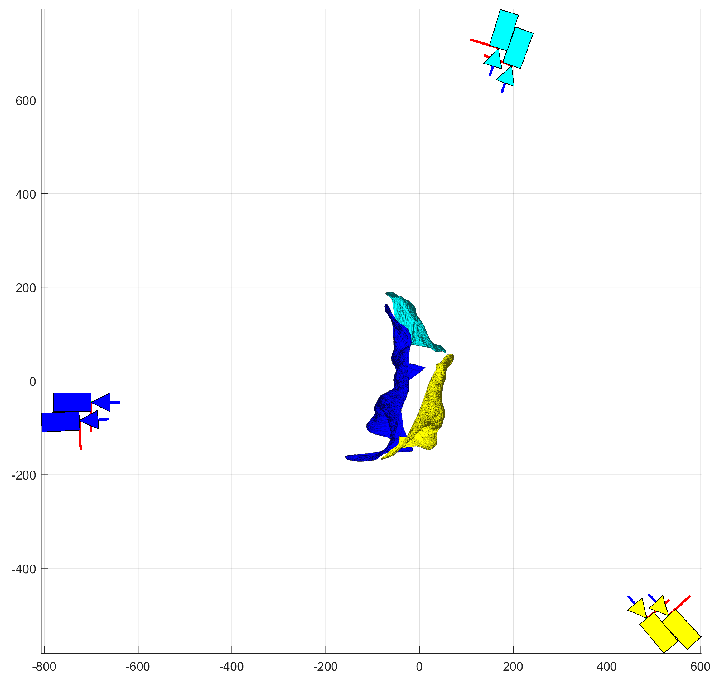
Triangulation and 3D filtering produces kT-sets of point clouds, XTR(k), for each kth stereo-camera pair. Each point cloud is then used to create a triangular surface patch, T(k), of the target object through a Delaunay triangulation. T(k) is herein defined as the triangulation map, wherein triangulation is the graphical subdivision of a planar object into triangles. The map is a size [npolys × 3] index matrix whose rows index the three points from XTR(k) that make up a given surface patch polygon. The surface patch is obtained by firstly projecting the point cloud into each camera’s image plane as a set of 2D pixel coordinates. One set of 2D coordinates is then triangulated using Delaunay triangulation. The triangulation map is then applied to the second set of 2D coordinates and checked for inconsistencies, such as incorrect edges. Incorrect edges are a symptom of incorrectly triangulated 2D features. The incorrect edges are removed by removing the 3D points in XTR(k) that connect to the most incorrect edges. The result is a set of fully filtered point cloud matrices XTR(k) and their associated surface patches, T(k), as shown in Figure 2.
3.5. Tracking
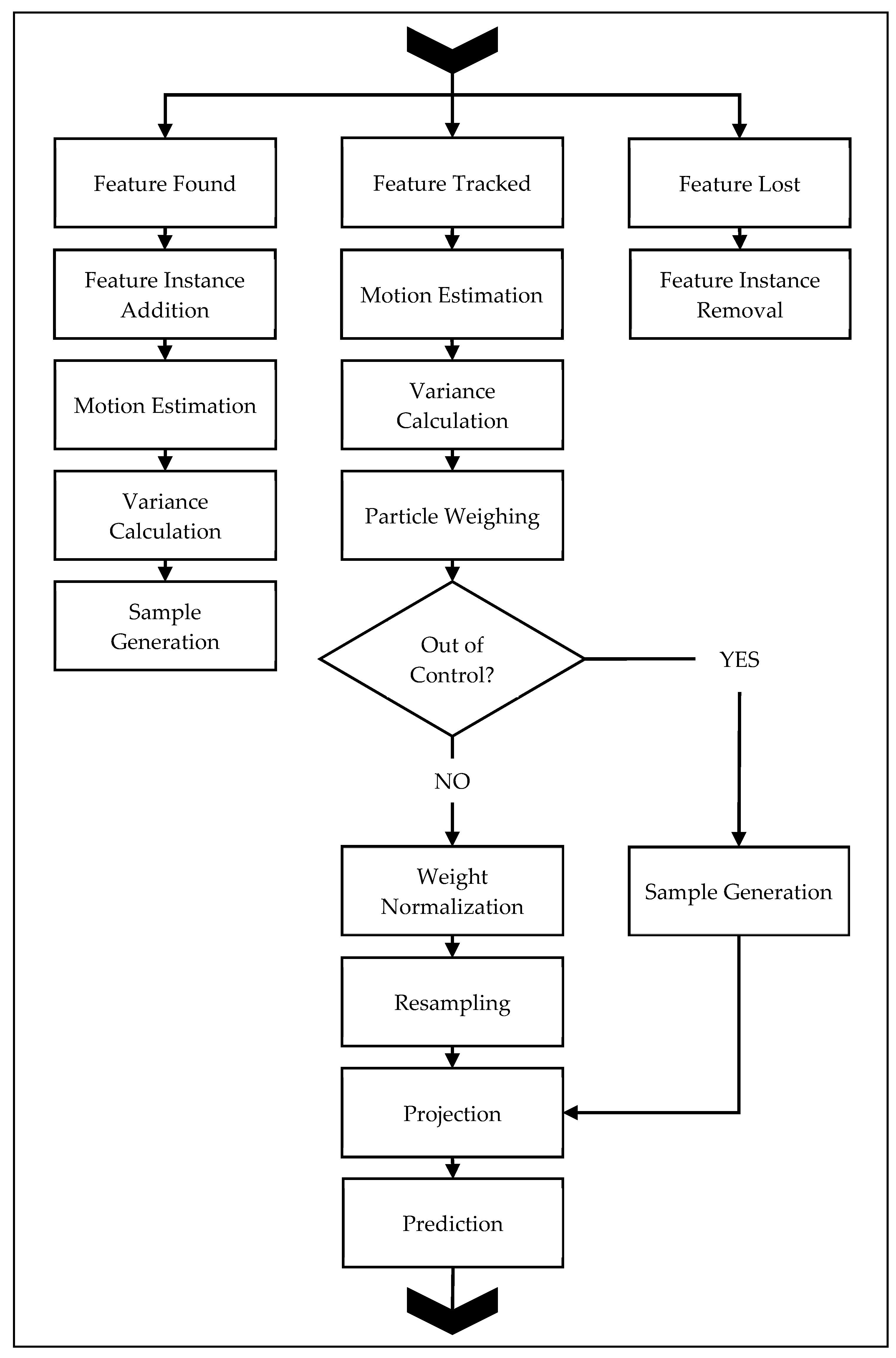
The tracking process implements 3D tracking-through-detection with a user-defined motion model. An unknown object implies an unknown motion model, which may be simple or complex. In order to set a standard complexity for the motion model, a constant-acceleration model was chosen for the tracking and prediction process. The benefit of the constant-acceleration model is its applicability to a range of target motions with limited data requirement, i.e., only three data samples are necessary for prediction. Alternative motion models are discussed at the end of the section. The complete filtering algorithm is presented in Figure 3, and consists of three major streams: feature found—the handling of new triangulated points, feature tracked—the handling of points that were located across multiple consecutive demand instants, and featurelLost—the handling of points that were previously located but were not located at the current demand instant.
The on-line adaptive particle filter loads the measurement data from the 3D database for the current and previous demand instants. Each 3D point from the previous demand instant is checked against the current set of 3D points based on the unique key-identifier assigned to them in triangulation to determine whether the point was tracked across demand instants. Three outcomes are possible: the point could have been tracked across demand instants, the point could have been lost, or the point is new.
Automatic initialization identifies all newly triangulated points, and allocates space for the necessary particles for tracking, and a state-space measurement history of the last five demand instants. This process works for tracking starting from Demand Instant 0, as all triangulated points will be labeled as new in comparison with other methods that require an a priori demand-instant measurement [3,14].
The feature found stream applies to all points detected in three or less consecutive demand instants. If the feature is only been detected in less than three consecutive instants, its state-space measurement is updated. Features triangulated in three consecutive demand instants have their motion estimated through a first- and second-order backward differencing operation.
where Δt is the change in time between demand instants, X(t) is the 3D positional measurement of the given point, Ẋ is the estimated velocity, and Ẍ is the estimated acceleration. The constant-acceleration model requires nine total states: three positions, three velocities, and three accelerations.
The total number of particles, q, is user-defined. The number of particles used determines the accuracy of the prediction at the cost of computational power [54]. The number of particles may be varied on-line based on the calculation of the total effective number of particles [54,72]. Herein, the number of particles was kept static throughout all demand instants to avoid dynamic memory reallocation tasks. Therefore, each particle filtering instance initialized is composed of a [9 × q] particle matrix. The particles are drawn from a normal distribution for each tracked point.
where xj* is the nine-dimensional state-vector of the jth tracked point, and is its associated variance. The measurement variance, , is set equal to the particle variance, to ensure the partiality weighing step also adapts on-line with varying deformation dynamics.
The particle variances are calculated as
which are updated with every measurement of a tracked point. The on-line updating of the variances ensures the particles remain within close proximity to the measurement. The initial set of particles is then generated given the motion model and the particle variance.
Points that are tracked for more than three consecutive demand instants are labeled as tracked and are processed through the feature tracked stream. As a new positional measurement becomes available at the current demand instant, the state-space measurement for a given point is calculated by Equations (8) and (9), and stored in the state-space measurement history. Thereafter, for each jth point, the set of projected particles Qj+ is loaded, and each nine-dimensional particle is weighed against the current state-space estimate xj*.
where Wj is the weight matrix of all particles for the jth point. The weights are then normalized.
The normalized weight matrix Wj* is of size [9 × q]. The summed term is checked for a zero-condition which occurs if the projection is too far off from the measured location. All states with a zero-sum condition bypass the resampling step, and new particles are generated from the most recent measurement. All remaining states with non-zero sums, i.e., states with accurate projections, are resampled through a sequential importance process [54]. The regenerated states and resampled states are combined into an updated Qj matrix.
3.6. Prediction
The prediction process relies on the user-defined motion model to correctly project the particles. The projection produces an estimate for all tracked particles’ poses for the consecutive demand instant. The prediction process occurs only in the tracked stream and follows the projection step. The projection step requires the updated particle matrix Qj, which is then projected to determine the expected state-space of the jth point at the next demand instant.
where Qj+ is the matrix of projected particles for the jth point, H is the [9 × 9] constant-acceleration state transition matrix, and U is the [9 × q] uncertainty matrix based on the particle projection variance (Equation (11)). The particle matrices are then averaged to produce a single state-space estimate of the predicted point.
The projected state-space points are stored into a predicted pose matrix X+. For each subset of tracked points from X+ detected by the ith camera pair, a surface mesh is applied. Thus, the resulting output of the methodology is a set of n meshes that represent the predicted deformation of the object. Figure 2 illustrates the predicted deformation of a dinosaur from three stereo-camera pairs where each colored surface patch correlates to a particular point-cloud prediction of the corresponding stereo pair.
Points that were previously detected and are lost at the current demand instant are labeled as lost, and are processed through the feature lost stream. The particle matrices and state-space measurement vectors associated with these points are removed from memory, but their unique key-identifiers remain, along with the associated 2D feature keys. Lost points that are detected anew in later demand instants are processed through the feature found stream.
The tracking and prediction task allows for modularity in the filtering methodology chosen, including particle filters, KFs [50], EKFs [73], unscented KFs [74], and PSO [55,57]. The particle filter was chosen due to its robustness to non-Gaussian noise [54,75], and its common-place implementation in tracking methodologies [76,77]. A KF may not necessarily work well since camera noise is non-Gaussian [78] and, thus, tracking may fail. EKFs and unscented KFs may be better suited than regular KFs for tracking as they do not explicitly depend on Gaussian process noise. PSO should function similarly to particle filtering methods, but would require an optimization step that filtering does not.
The motion model may be user-selected as well for specific tasks, if necessary. The constant-acceleration motion model may be replaced with another simpler or more complex model. A constant-velocity model would decrease the state-space size required and the number of initial tracking demand instants with lower accuracy prediction. A Fourier series model may be used for objects that would undergo cyclic motion [58,79]. One can note that the motion model selected would dictate the total number of demand instants required before an accurate prediction could be made. For example, a constant-velocity model only requires two demand instants, while a constant-acceleration model requires three. The constant-acceleration model was chosen herein as a generalized approach for tracking due to its robustness to capturing human motion and certain non-linear motions.
4. Simulations
Extensive simulations were carried out using the Blender™ software [80] for object animation and camera representation. The VLFeat™ [81] library was used for image processing. MatLab™ was used to code the complete methodology. Six example simulations are presented herein to demonstrate the proposed methodology. Each simulation utilized a fixed stereo-camera pair.
All simulated camera models used a 32 × 18 mm Advanced Photo System type-C (APS-C) style sensor, with an image resolution of 1920 × 1080 pixels, and a focal length of 18 mm. Uniformly distributed color pixel noise was added to all images to simulate image noise. Furthermore, all triangulated data incorporated noise to simulate real-world errors in camera placement. The simulations used singular, textured object surfaces that deformed over a set of demand instants.
Three error metrics were used to analyze the performance of the methodology. The triangulation errors, et, were calculated as the Euclidean distance between a triangulated point and the nearest ground-truth surface. The prediction errors, ep, were calculated as the Euclidean distance between a predicted point and the nearest ground-truth surface. The relative prediction errors, ef, were calculated as the Euclidean distance between a predicted point locations and its actual triangulation location, for all tracked points. All three errors were normalized by the square root of the object’s surface area. The normalization ensures the error metrics are invariant to the size of the target object, and relative pose of the cameras.
Triangulation errors were calculated as follows:
where zt(j) is the shortest distance between the jth triangulated point in X to the surface of the true object model, m is the total number of triangulated points at the given demand instant, and S is the surface area of the true object model.
Prediction errors were calculated as follows:
where zp is the shortest distance between the jth predicted point in X+ to the surface of the true object model, and m is the total number of predicted points.
The relative prediction errors were calculated as follows:
4.1. Simulation 1
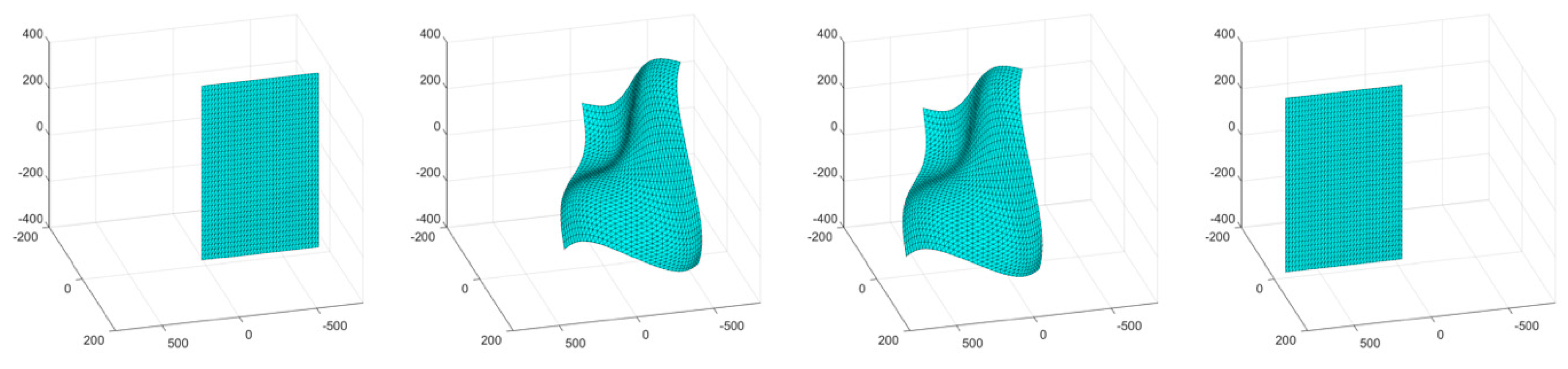
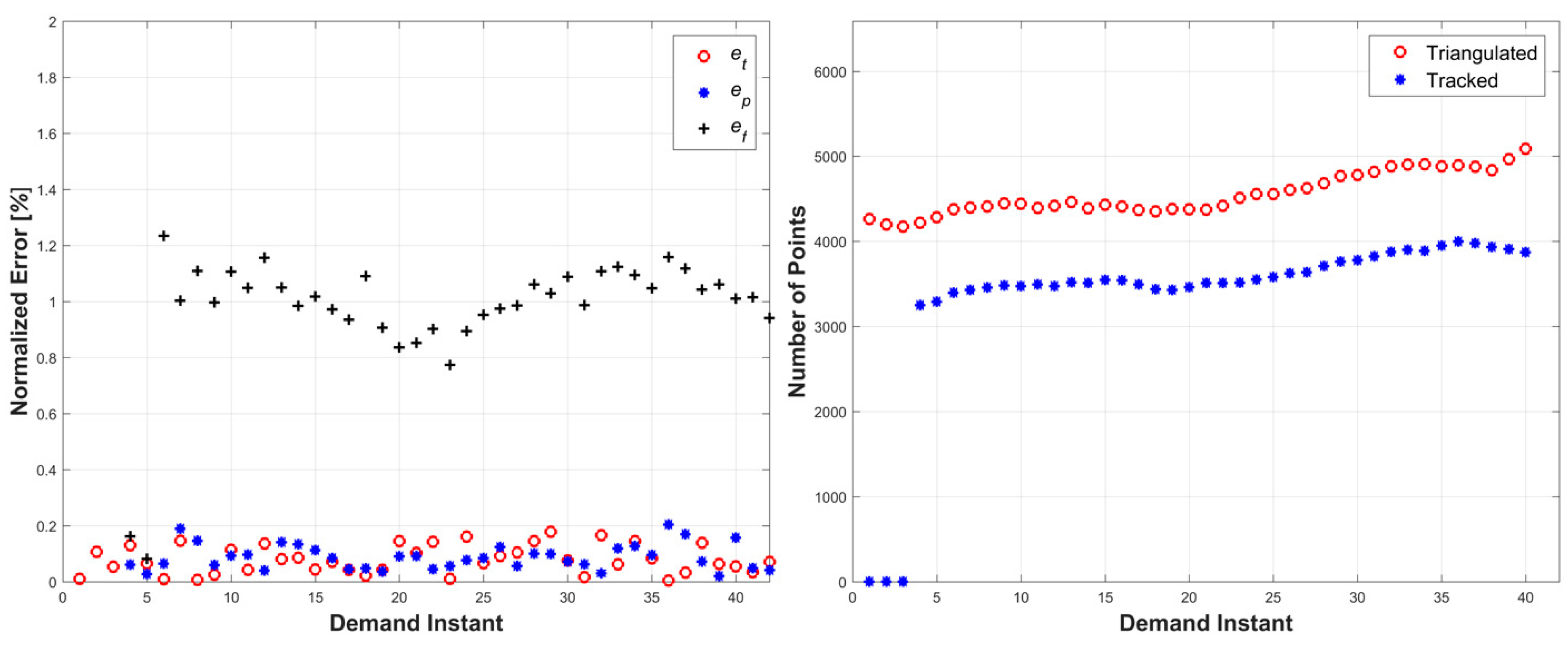
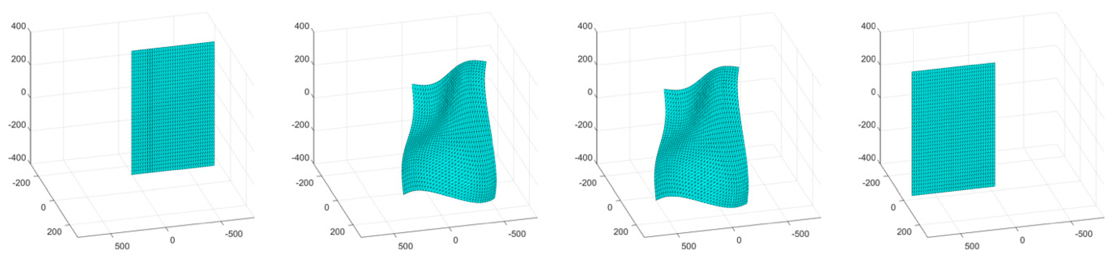
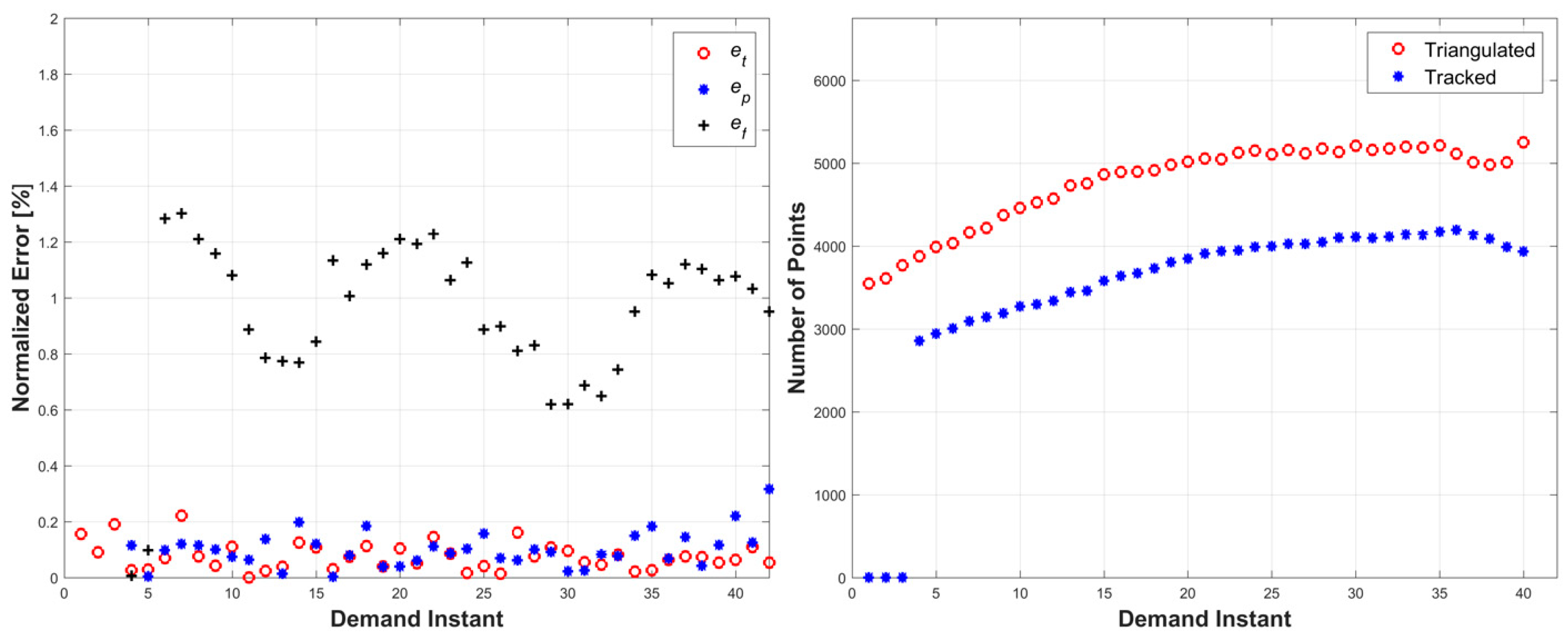
The first simulation consisted of an object surface undergoing a wave-like stretching deformation with a linear translation. A four-frame movie-strip of the object is presented in Figure 4. This simulation tested the methodology’s ability to handle a more complex form of surface deformation with global motion. The errors remained under 1.3% for all three error metrics, and the total number of tracked and triangulated points remained fairly stable with a slight increase (Figure 5). The slight increase in error from the third simulation is attributed to the compounded motion experienced by every tracked and triangulated point. Specifically, in the previous simulation, the tracked points only moved in the wave motion, while, in this example, they also moved perpendicularly to the wave motion, thus increasing the relative prediction errors.
4.2. Simulation 2
The second simulation consisted of an object surface undergoing a wave-like stretching with linear translations in two directions. A four-frame movie-strip of the object is presented in Figure 6. This simulation tested the methodology’s ability to handle a more complex form of surface deformation with increased global motion. The errors remained under 1.4% for all three error metrics, and the total number of tracked and triangulated points gradually increased as the object moved closer to the cameras (Figure 7). The cyclic error pattern for the relative prediction errors, ef, is attributed to the acceleration profile of the motion where the lowest error values correspond to zero acceleration of the object.
4.3. Simulation 3
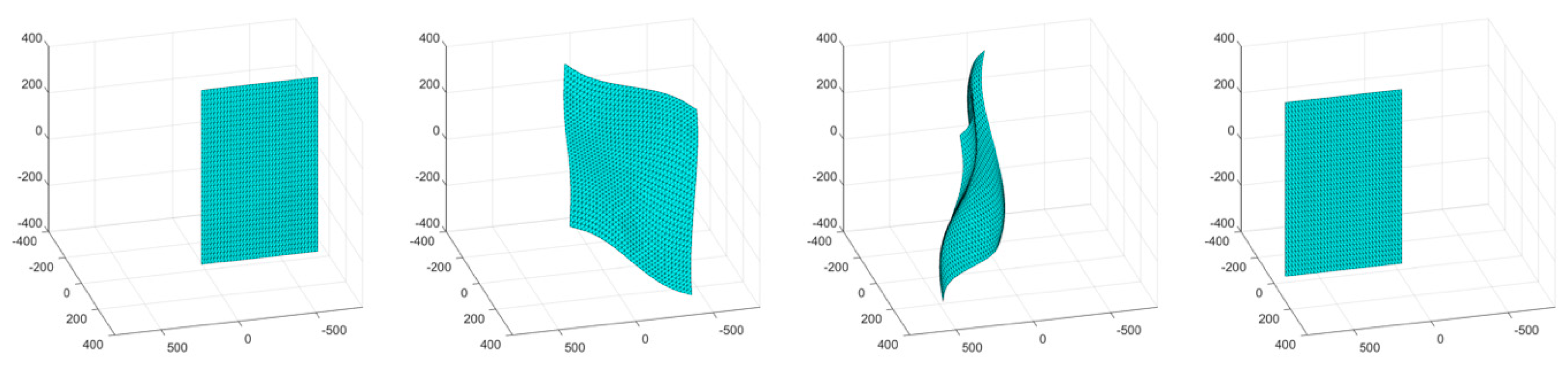
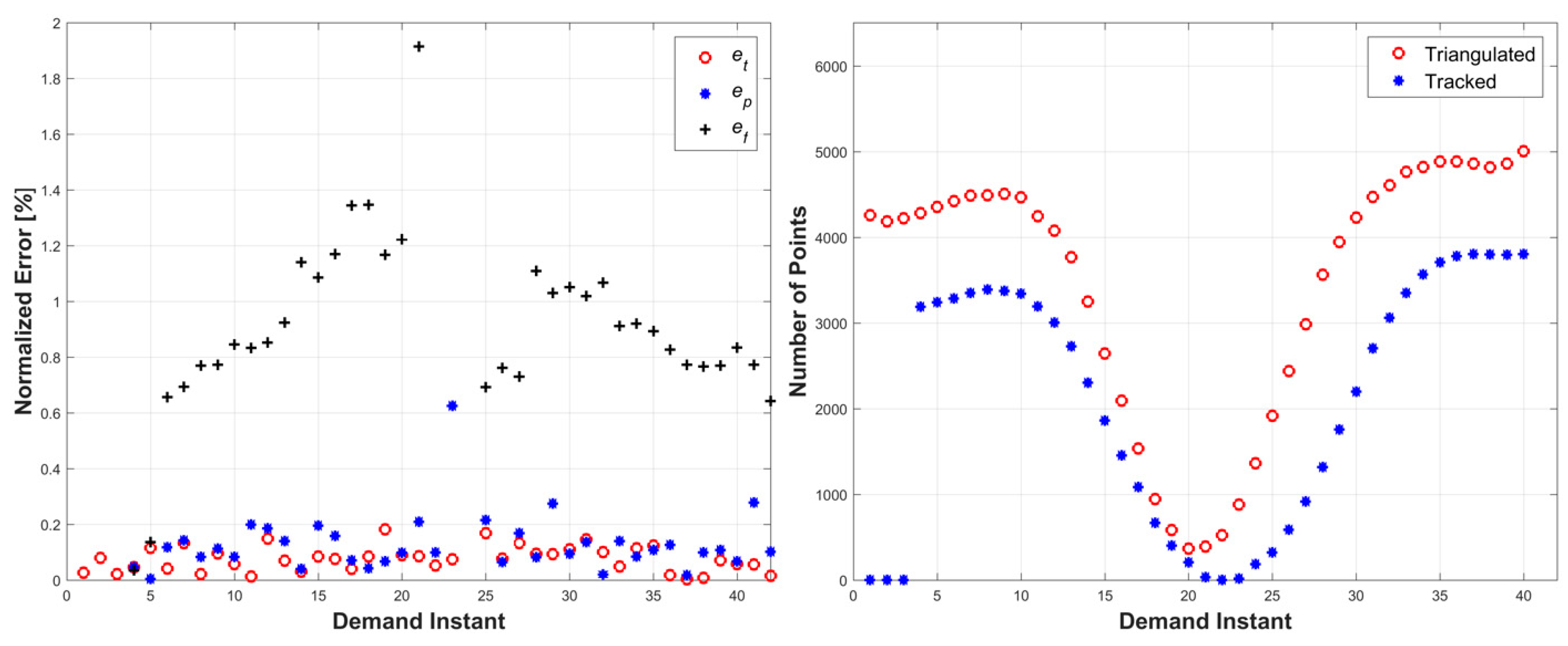
The third simulation consisted of a surface object undergoing a wave-like stretching with a linear translation and a rotation by 180°. A four-frame movie-strip of the object is presented in Figure 8. This simulation tested the methodology’s ability to handle complex surface deformation with complete loss of visibility. The errors remained under 2% for all three error metrics, with an increasing trend as the object rotated to a parallel orientation with respect to the cameras, at which point none of the triangulated points could be tracked (due to loss of tracking data) (Figure 9). The number of tracked and triangulated points reflected the error behavior. Specifically, as the object became parallel to the cameras, the number of triangulated points decreased to almost zero, while all of the tracked points were lost.
5. Experiments
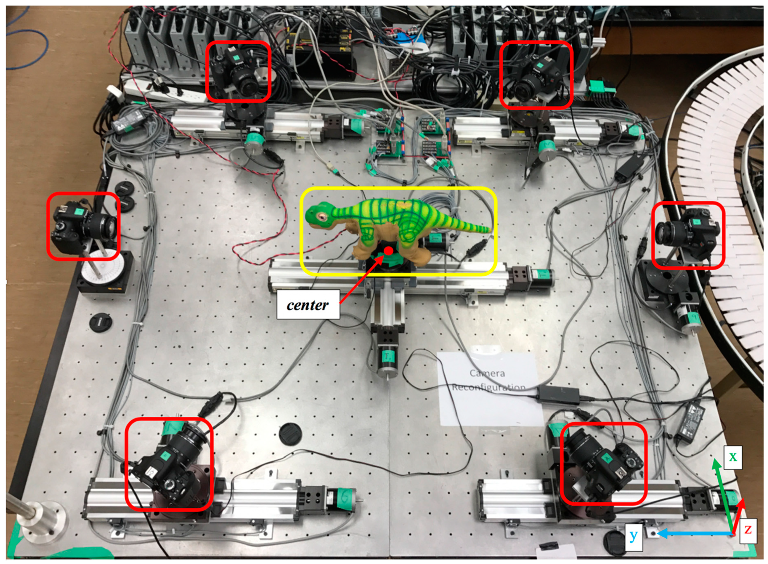
Experiments were conducted using a robotic deformable object, namely the PleoRB robot, as the target object. The experimental platform was composed of six calibrated Canon digital single-lens reflex (DSLR) Rebel T3i cameras, and one Intel i7 personal computer (PC) with 24 GB of RAM. The general layout of the experimental set-up is presented in Figure 10 with the mobile cameras and the robot (deformable object) highlighted. As shown in the figure, all six cameras were placed on moving stages to attain any desired reconfiguration. Two cameras were placed on one-degree-of-freedom rotational stages, whereas the other four cameras were placed on two-degree-of-freedom stages—rotational and translational. During the experiments presented in this paper, only three two-degree-of-freedom cameras were utilized.
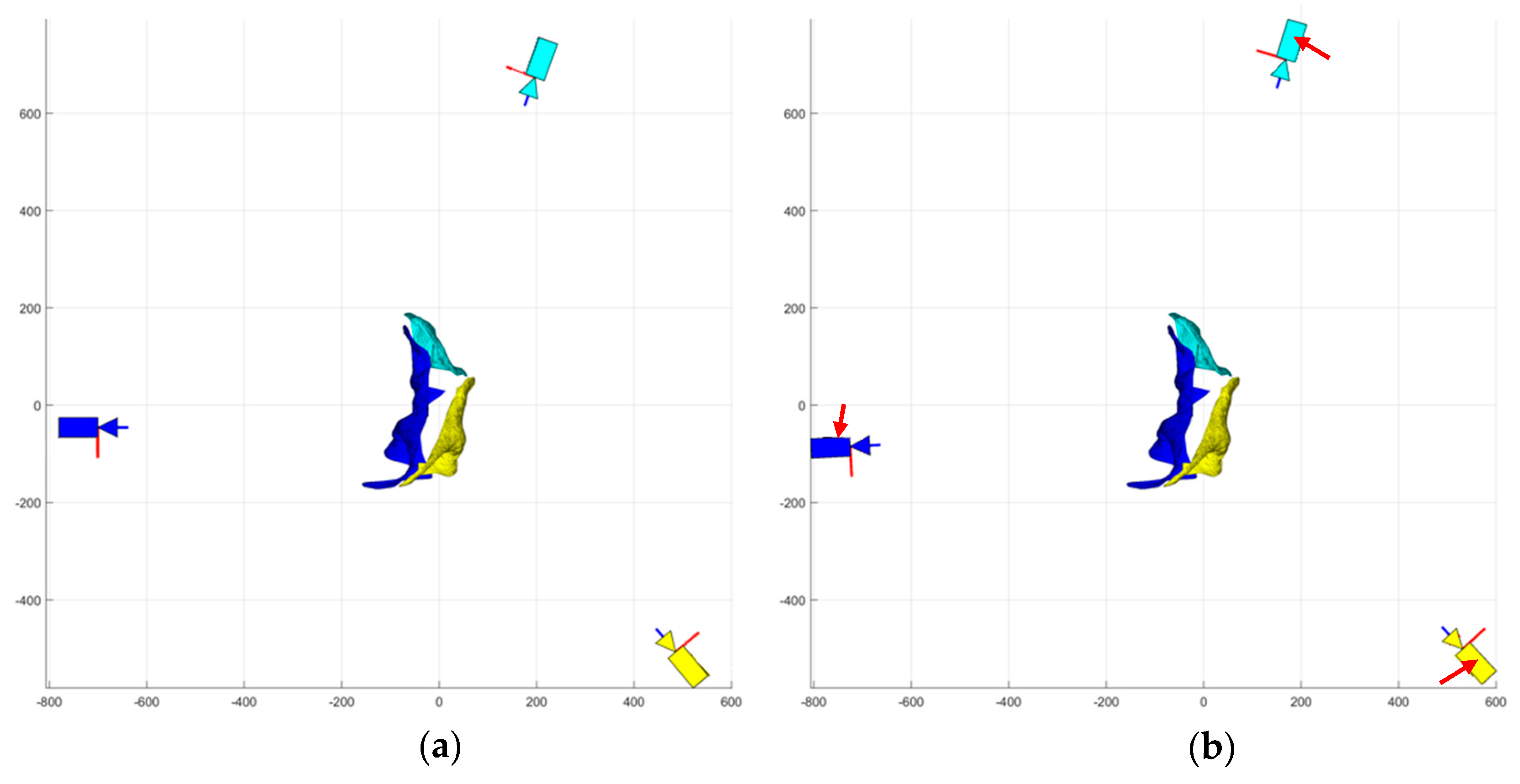
As noted above, the initial experimental configuration presented in Figure 10 could not provide the desired static stereo-camera placement. Therefore, in order to achieve the desired configuration, as in Figure 2, the experiments had to be conducted quasi-dynamically. Specifically, for a given demand instant, once the robot was moved and deformed into its desired surface, three two-degree of freedom cameras were moved into their first stereo-pair position (circular pattern, 120° separation) and captured their respective images (Figure 11a). Next, the cameras were moved on an arc of 100 mm to their second stereo-camera positions and captured their respective second images (Figure 11b). The robot was then deformed into its next pose of the sequence and the quasi-dynamic capture process was repeated. Thus, each object’s deformation required the reconfiguration of three of the four cameras to simulate stereo pairs.
The cameras were calibrated at fixed optical parameters, namely focal length, aperture, shutter speed, and image gain. The camera settings were chosen to maximize image sharpness and ensure correct depth of field. The average distance between the robot and each camera was 775 mm. The cameras were all electronically controlled through Universal Serial Bus (USB) using Canon’s camera control software development kit (SDK): EDSDK.
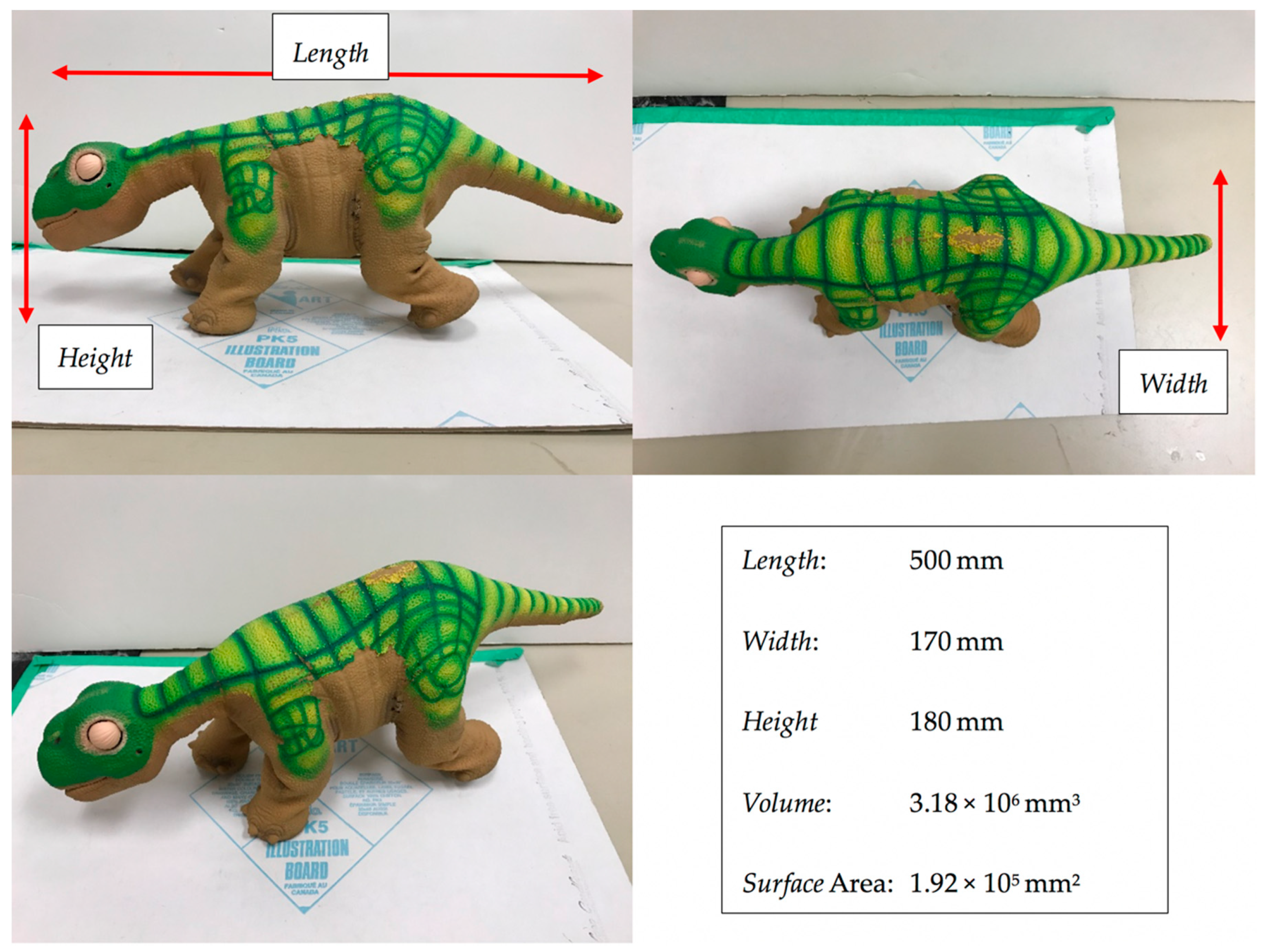
The target object, PleoRB robot, was chosen due to its surface texture and high degree-of-freedom (DOF) configuration (Figure 12). The robot was composed of 15 servo motors actuating the mechanical armatures with a patterned texture rubber skin. The PleoRB robot was controlled through serial USB. A custom program was developed to individually set each servo motor’s position, ensuring repeatability. The volume and surface area of the robot were calculated manually by measuring each limb individually and approximating limbs with geometric objects such as cylinders, cones, and rectangles.
5.1. Background Segmentation
Background segmentation was outside of the scope of this work; however, it is a necessary aspect of the system for correct deformation estimation. The development of generic target segmentation algorithms is a field of computer vision in and of itself, with several notable examples available in References [82,83,84,85].
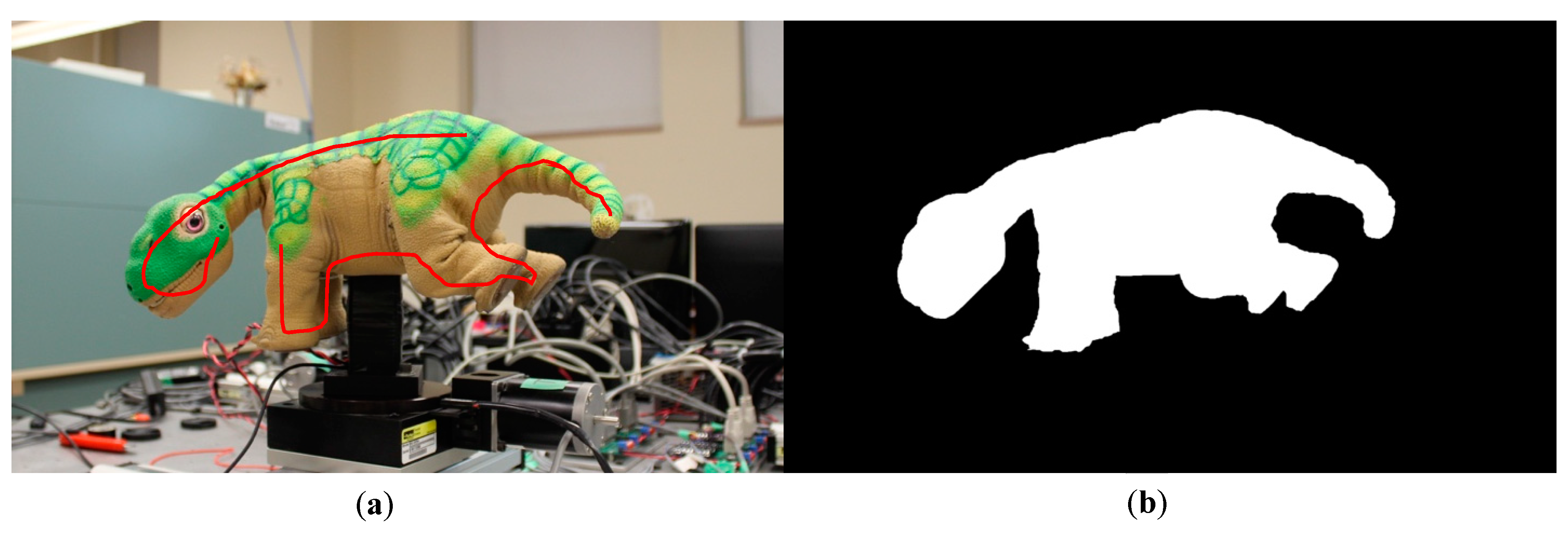
In order to overcome the problem of target segmentation, a run-time implementation of Grabcut was integrated into the process to segment the target object from the noisy background [86]. The Grabcut method implements a graph-cut energy-minimization problem solved via maximum flow through a graph. The Grabcut process consists of the user providing a set of guide points on the input image that are near the target’s boundary. The algorithm then solves for the image boundary that optimizes the max-flow min-cut problem. The output of the algorithm is a binary image mask that labels the pixels as background or target (Figure 13).
5.2. Results
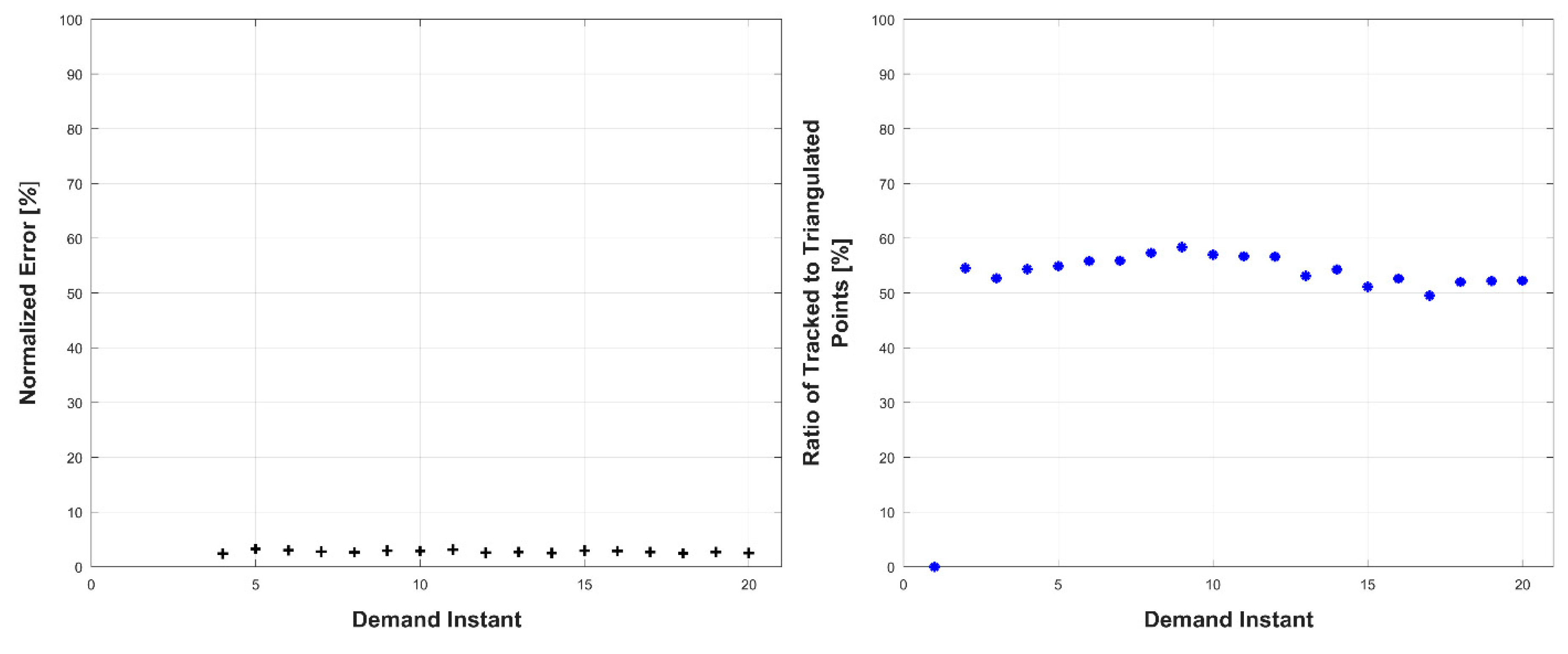
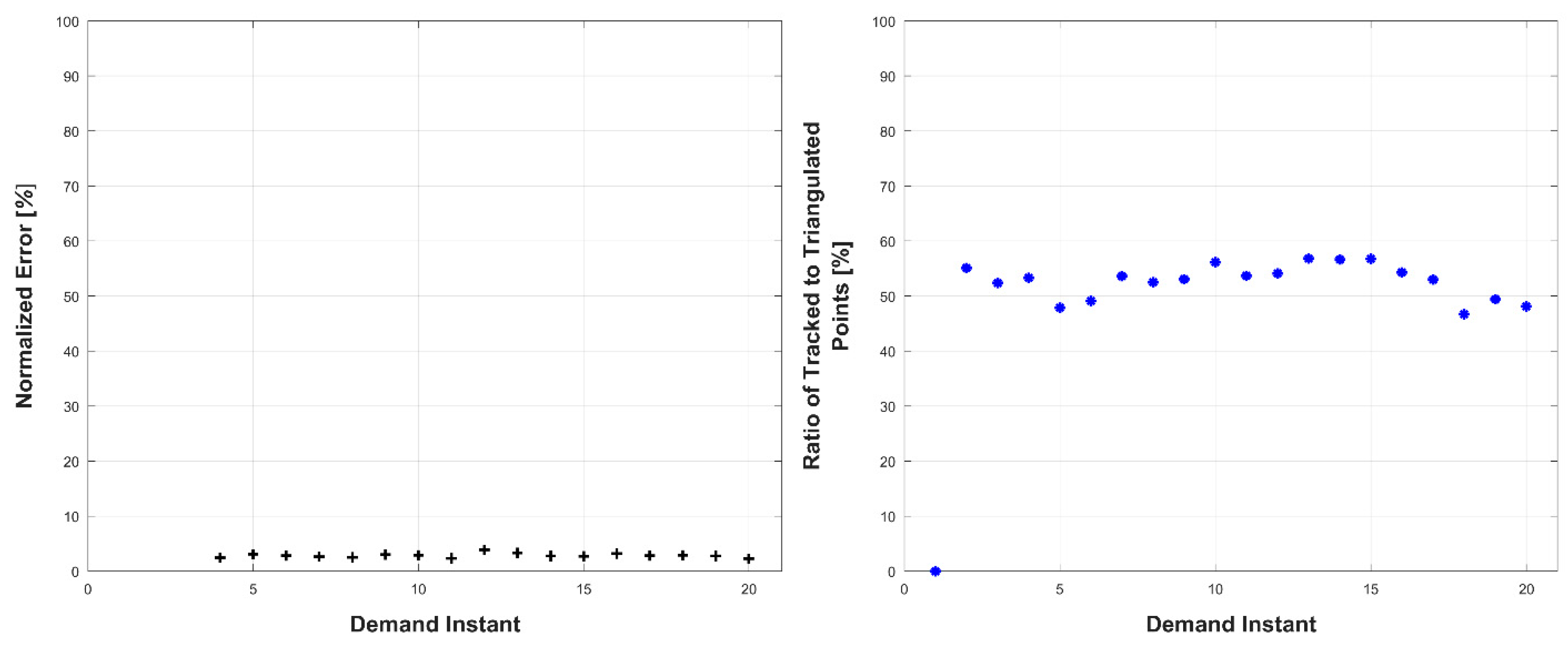
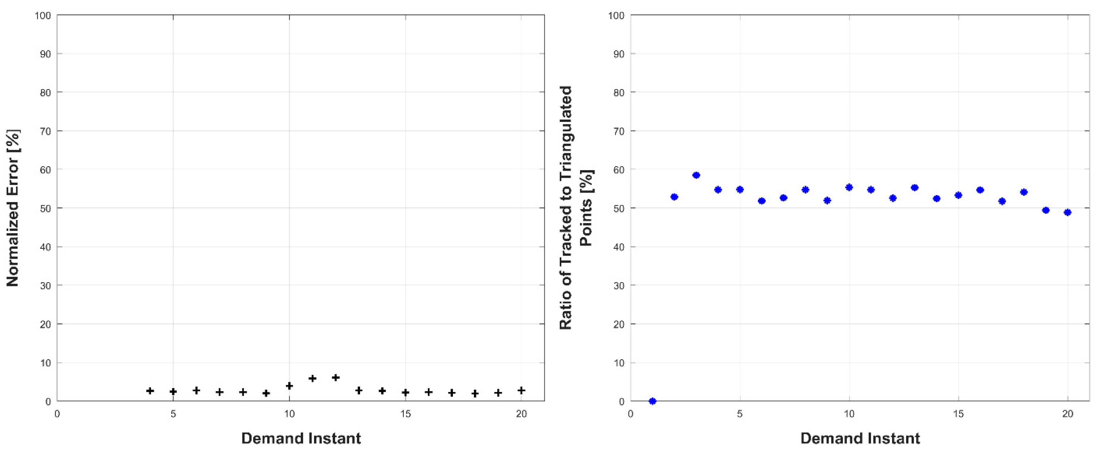
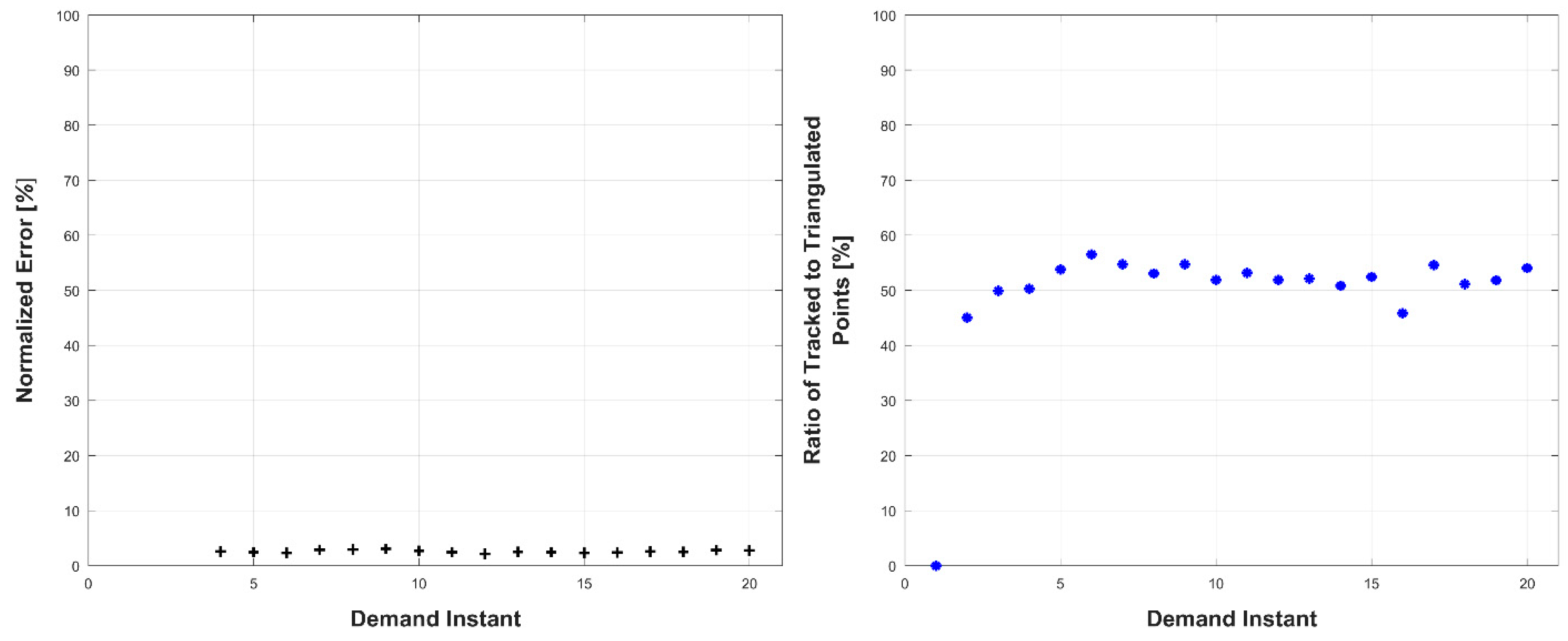
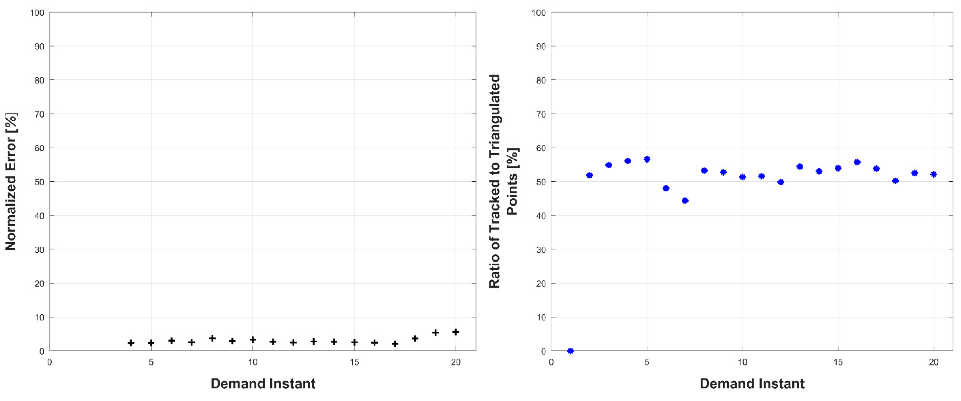
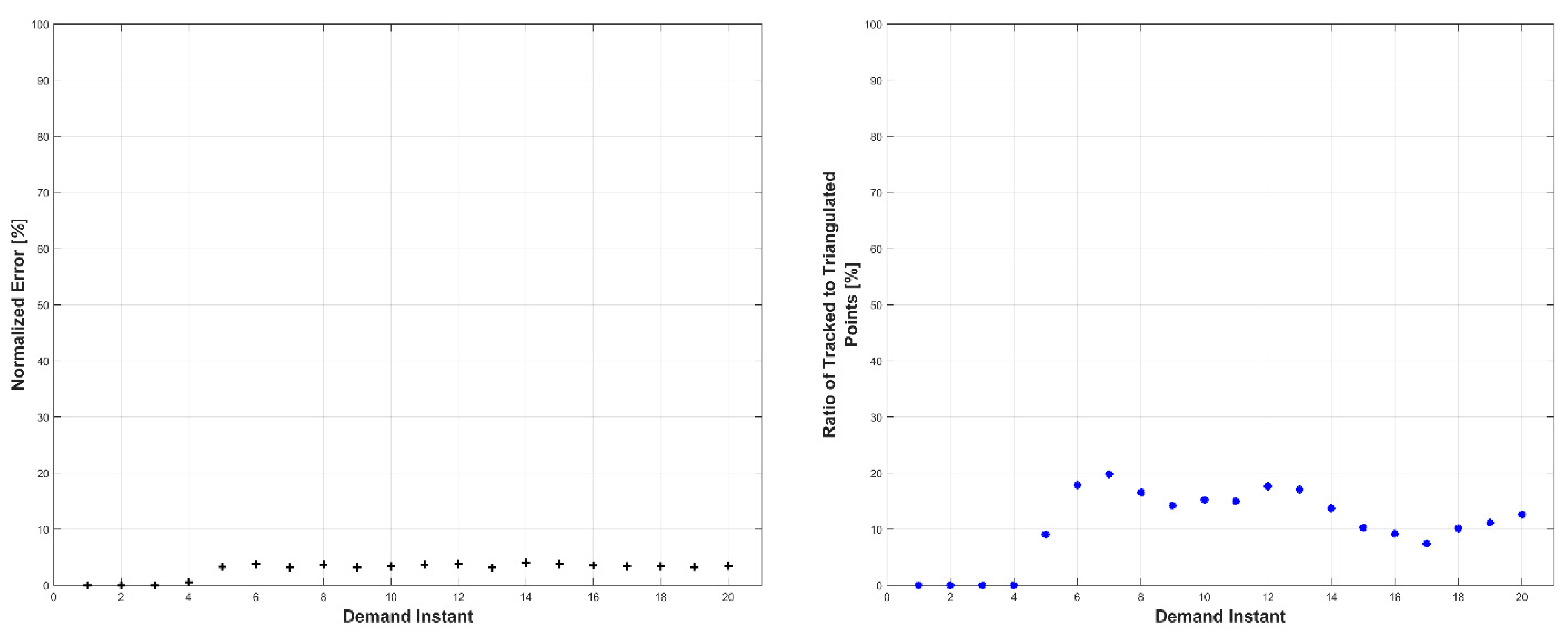
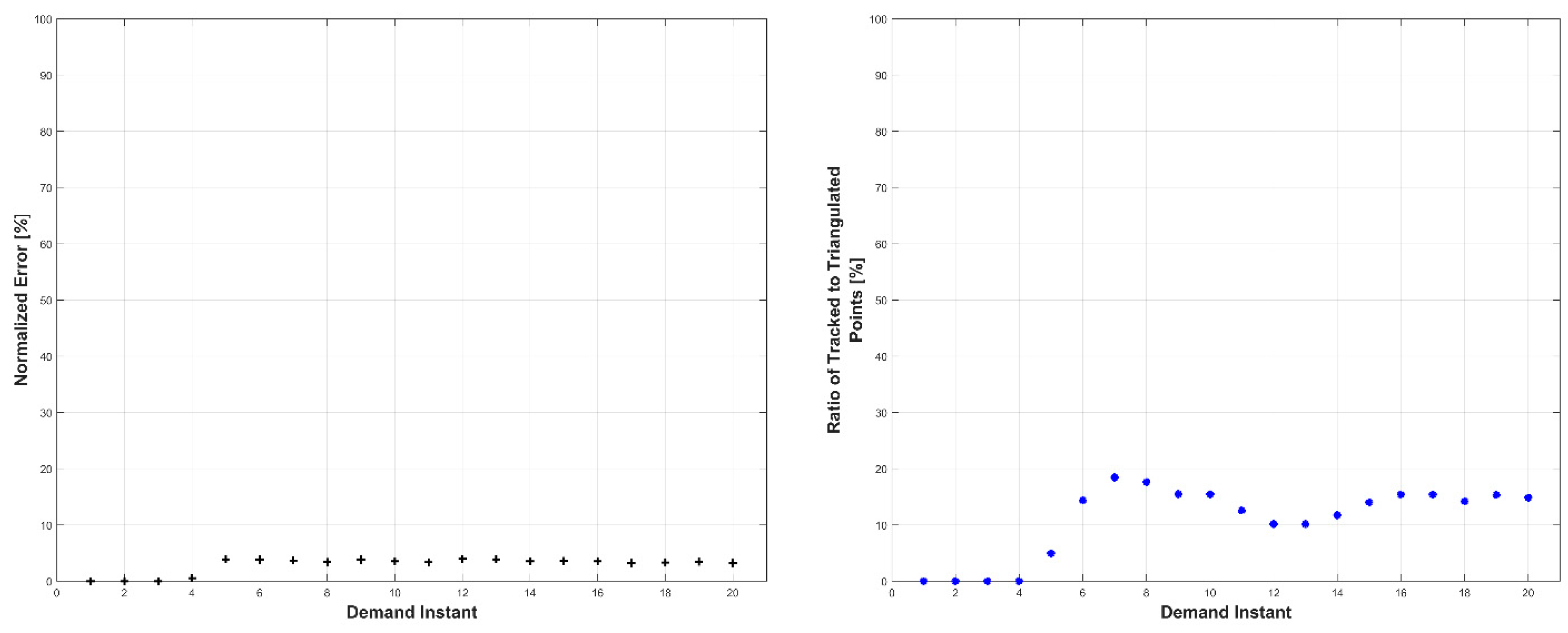
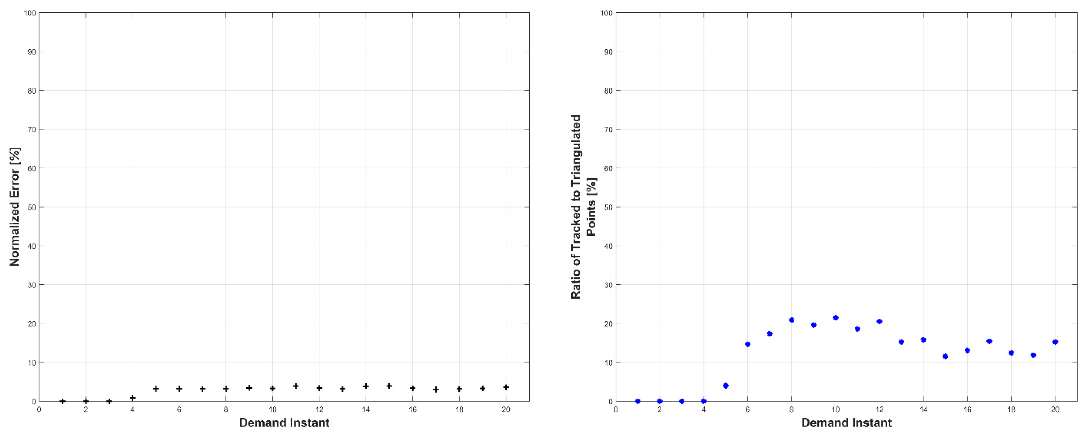
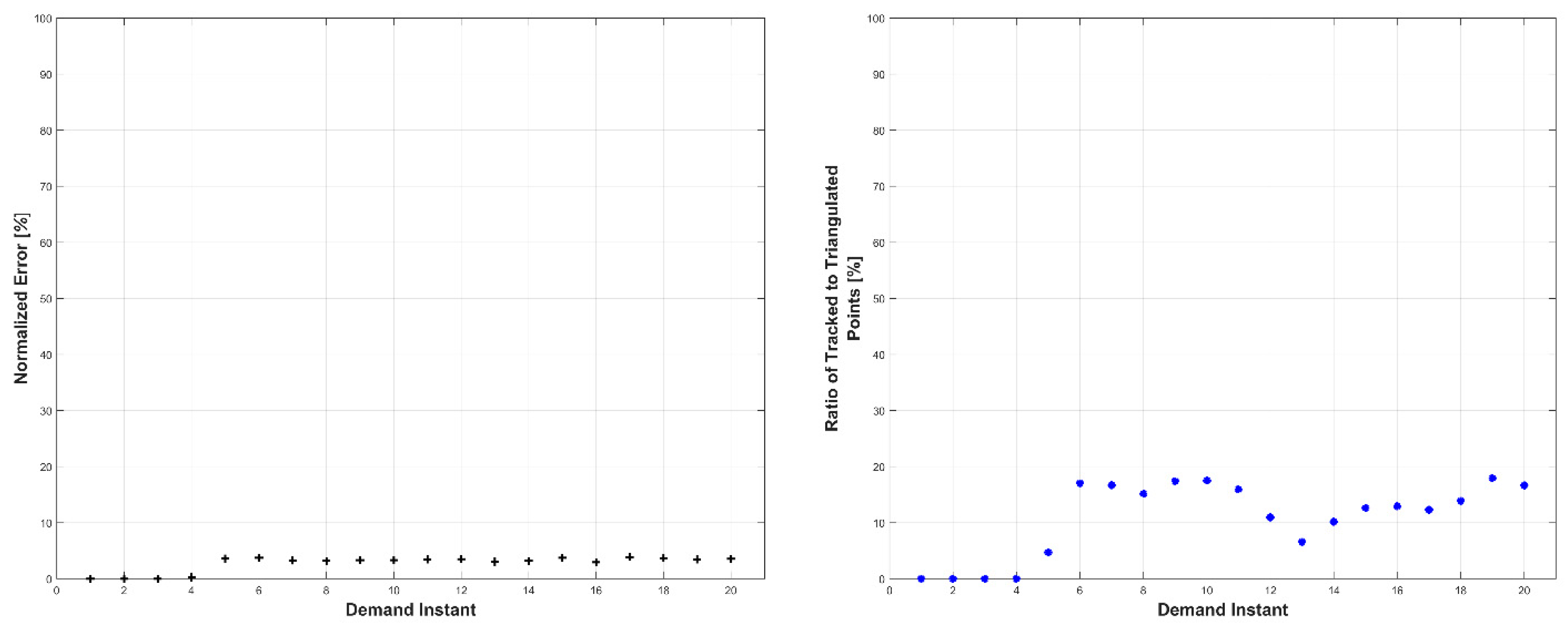
Experiments were conducted in two sets: occluded and unoccluded. The cameras were placed into three stereo pairs separated by 120° about the center of the robot. The robot deformed over a set of 20 demand instants. The unoccluded set of experiments consisted of five robot deformations without dynamic obstacles. The occluded set of experiments consisted of the same five deformations, but with a dynamic obstacle moving through the workspace partially occluding one pair of cameras.
The results, presented below in Figure 14, Figure 15, Figure 16, Figure 17, Figure 18, Figure 19, Figure 20, Figure 21, Figure 22 and Figure 23, indicate the performance of the deformation estimation methodology when applied to a real-world scenario. In the case of both the occluded and unoccluded experiments, the methodology was capable of predicting the expected deformation of surface patches with less than 4% error. The major difference between the occluded and unoccluded results is the ratio of tracked to triangulated point at each demand instant. Specifically, in the unoccluded case, all three camera pairs triangulate and track a large portion of the target object resulting in an even ratio of tracked to triangulated points. Conversely, in the occluded case, the obstacle results in a large loss of triangulated and tracked points visible by one of the camera pairs; thus, the ratio of tracked to triangulated points is reduced. Movie-strip representations of the predicted surface deformations for one experiment from each occluded and unoccluded set are provided in Appendix A for reference. Similarly, a movie-strip view of the predicted surface patch deformations alongside the camera views are provided for all unoccluded experiments in Appendix B.
The average processing times per demand instant for each experiment are presented in Table 1. It is noted that the image processing of each stereo pair was parallelized in software. All code was written in MatLab without specific optimization.
Unoccluded Experiments
Occluded Experiments
6. Conclusions
This paper presents a novel, modular, multi-camera method for deformation estimation of unknown, markerless 3D objects. We showed that the modular methodology is capable of accurate surface-deformation estimation of the target object under varying motions. The proposed method presents an approach for deformed shape estimation up to scale. Camera calibration could upgrade certain existing state-of-the-art methods with scale information; however, generally, there is no single method that could become comparable with a camera-calibration upgrade. Specifically, model-based methods would have an advantage of the model for optimized fitting, while monocular methods would require an update with a secondary camera, and the introduction of scaled triangulation, which would become the proposed method. Therefore, it is not possible to explicitly compare the proposed method with the existing state of the art without upgrading the latter to achieve the same objective as the proposed method.
The methodology uses an initial stereo-camera selection process. It is noted that, for the purposes of the simulations and experiments presented in this paper, the cameras were manually positioned, resulting in a trivial stereo-pair selection. Then, for each demand instant, images were captured for all cameras and a set of SIFT features were located in each image. The SIFT features were matched between each camera pair, and filtered to remove outliers. Stereo triangulation yielded a set of 3D points which were further filtered to remove outliers. The 3D points were tracked and projected through an adaptive particle filtering framework. Adaptive filtering allows for a varying number of tracked 3D points, and modifies tracking parameters on-line to ensure maximal accuracy in prediction. A constant-acceleration motion model ensures accurate tracking for large variations in tracked objects. The numerous simulations and experiments presented herein were used to validate the methodology. The results demonstrate the methodology’s robustness to varying types of motion, and its ability to estimate deformation even under large tracking losses in both completely controlled environments and real-world environments.
Author Contributions
Conceptualization, E.N. Data curation, E.N. Formal analysis, E.N. Funding acquisition, B.B. Investigation, E.N. Methodology, E.N. Project administration, B.B. Resources, B.B. Software, E.N. Supervision, B.B. Validation, E.N. Visualization, E.N. Writing—original draft, E.N. Writing—review and editing, B.B.
Acknowledgments
The authors would like to acknowledge the support received, in part, by the Natural Sciences and Engineering Research Council of Canada (NSERC).
Conflicts of Interest
The authors declare no conflicts of interest.
Nomenclature
| Total number of cameras. | |
| State transition matrix, [9 × 9]. | |
| Matrix of stereo camera pairs, [2 × kv]. | |
| Matrix of camera combination pairs, [2 × kmax]. | |
| Set of particles, [9 × q]. | |
| Set of projected particles, [9 × q]. | |
| True surface area for the object model. | |
| Triangulation of all individual surface patches. | |
| Uncertainty matrix for tracking and prediction, [9 × n]. | |
| Vectors between given SIFT feature and its nearest neighbors in the left image, [2 × n]. | |
| Vectors between given SIFT feature and its nearest neighbors in the right image, [2 × n]. | |
| Weight matrix for all particles of the jth tracked point, [9 × q]. | |
| Normalized weight matrix for all particles of the jth tracked point, [9 × q]. | |
| Matrix of all triangulated points’ poses, [3 × n]. | |
| Matrix of triangulated points’ poses for a single stereo-camera pair, [3 × n]. | |
| Matrix of all tracked, triangulated points’ estimated velocities, [3 × n]. | |
| Matrix of all tracked, triangulated points’ estimated accelerations, [3 × n]. | |
| Predicted pose of all tracked, triangulated points, [3 × n]. | |
| Baseline separation between ith camera pair. | |
| Maximum baseline separation for a camera pair. | |
| Maximum epipolar distance. | |
| Euclidean lengths of each vector in VL, [n × 1]. | |
| Euclidean lengths of each vector in VR, [n × 1]. | |
| Normalized dL vector, [n × 1]. | |
| Normalized dR vector, [n × 1]. | |
| Normalized Euclidean distance error between triangulated points’ poses and the true object’s surface. | |
| Normalized Euclidean distance error between predicted points’ poses and the true object’s surface. | |
| Normalized Euclidean distance error between predicted points’ poses and the triangulated points’ poses. | |
| Total number of stereo-camera pairs. | |
| Total number of camera pairs possible. | |
| Optical axis vector for the cth camera, [3 × 1]. | |
| Total number of particles. | |
| Demand instant. | |
| Space-state vector of the jth tracked, triangulated point, [9 × 1]. | |
| Projected space-state estimate of the jth tracked, triangulated point, [9 × 1]. | |
| Euclidean distance between the jth tracked, triangulated point to the nearest true object surface coordinate. | |
| Euclidean distance between the jth predicted, tracked, triangulated point to the nearest true object surface coordinate. | |
| Change in time between demand instants. | |
| Angular separation between the jth camera pair. | |
| Maximum angular separation for a camera pair. | |
| Total number of cameras. | |
| State transition matrix, [9 × 9]. | |
| Matrix of stereo camera pairs, [2 × kv]. | |
| Matrix of camera combination pairs, [2 × kmax]. | |
| Set of particles, [9 × q]. | |
| Set of projected particles, [9 × q]. | |
| True surface area for the object model. | |
| Triangulation of all individual surface patches. | |
| Uncertainty matrix for tracking and prediction, [9 × n]. | |
| Vectors between given SIFT feature and its nearest neighbors in the left image, [2 × n]. | |
| Vectors between given SIFT feature and its nearest neighbors in the right image, [2 × n]. | |
| Weight matrix for all particles of the jth tracked point, [9 × q]. |
Appendix A
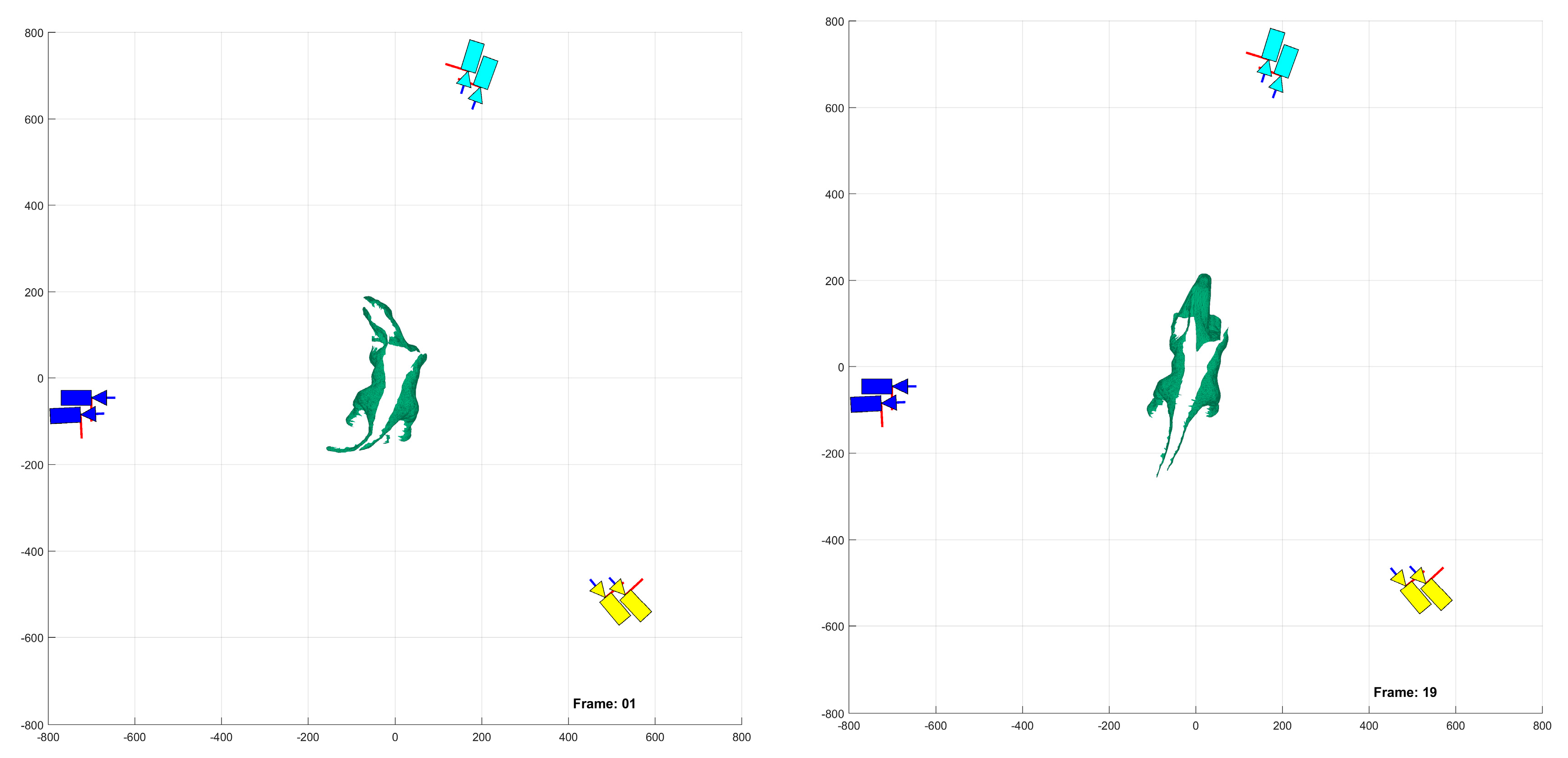
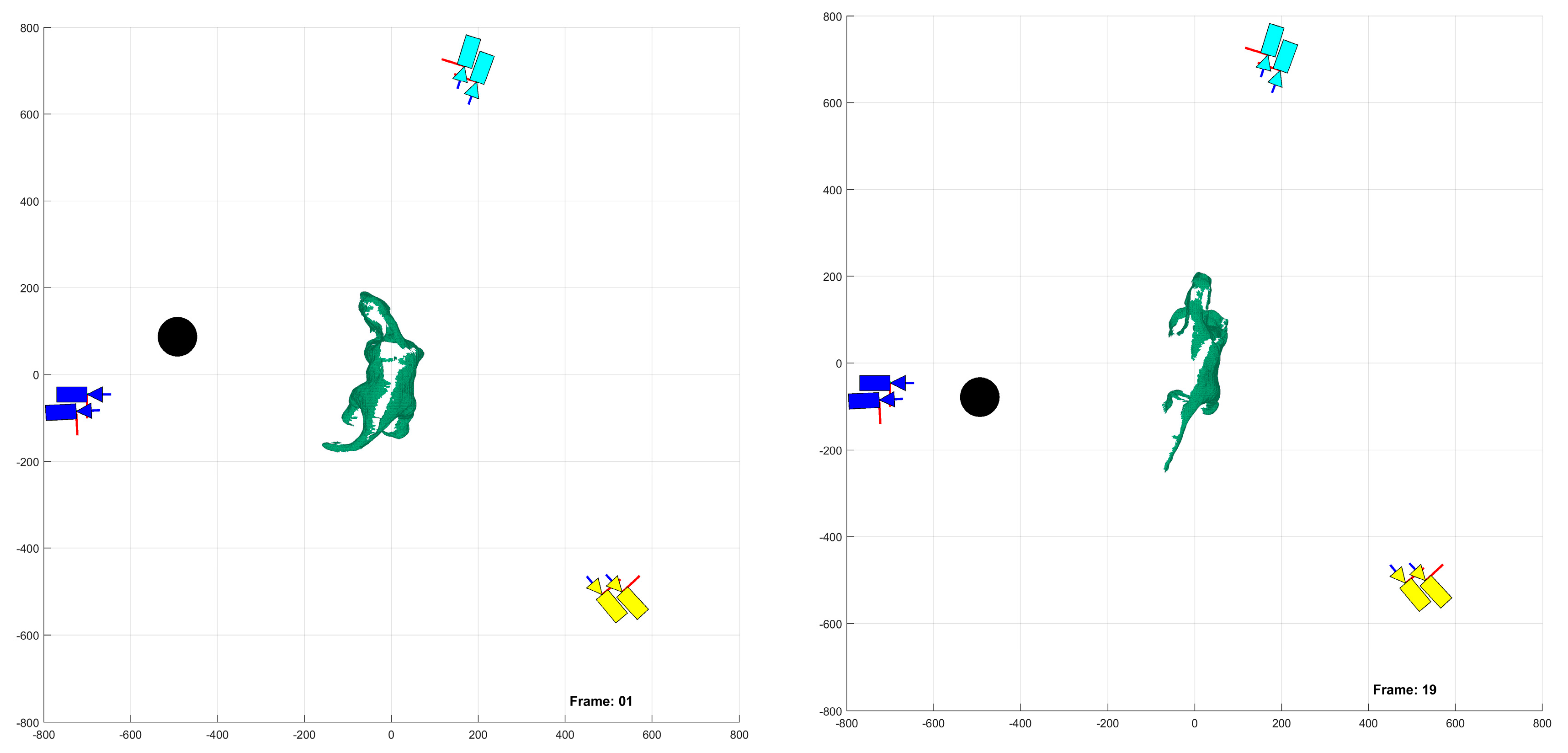
The following figures provide a bird’s-eye view of the experimental platform and predicted target object deformation as captured by all three camera pairs. The first set in Figure A1 corresponds to the first and last demand instants of an unoccluded experiment, while the second set in Figure A2 corresponds to the first and last demand instants of an occluded experiment.
Figure A1.
Unoccluded experiment demand instants 1 and 19, units in [mm].

Figure A2.
Occluded experiment demand instants 1 and 19, units in [mm].

Appendix B
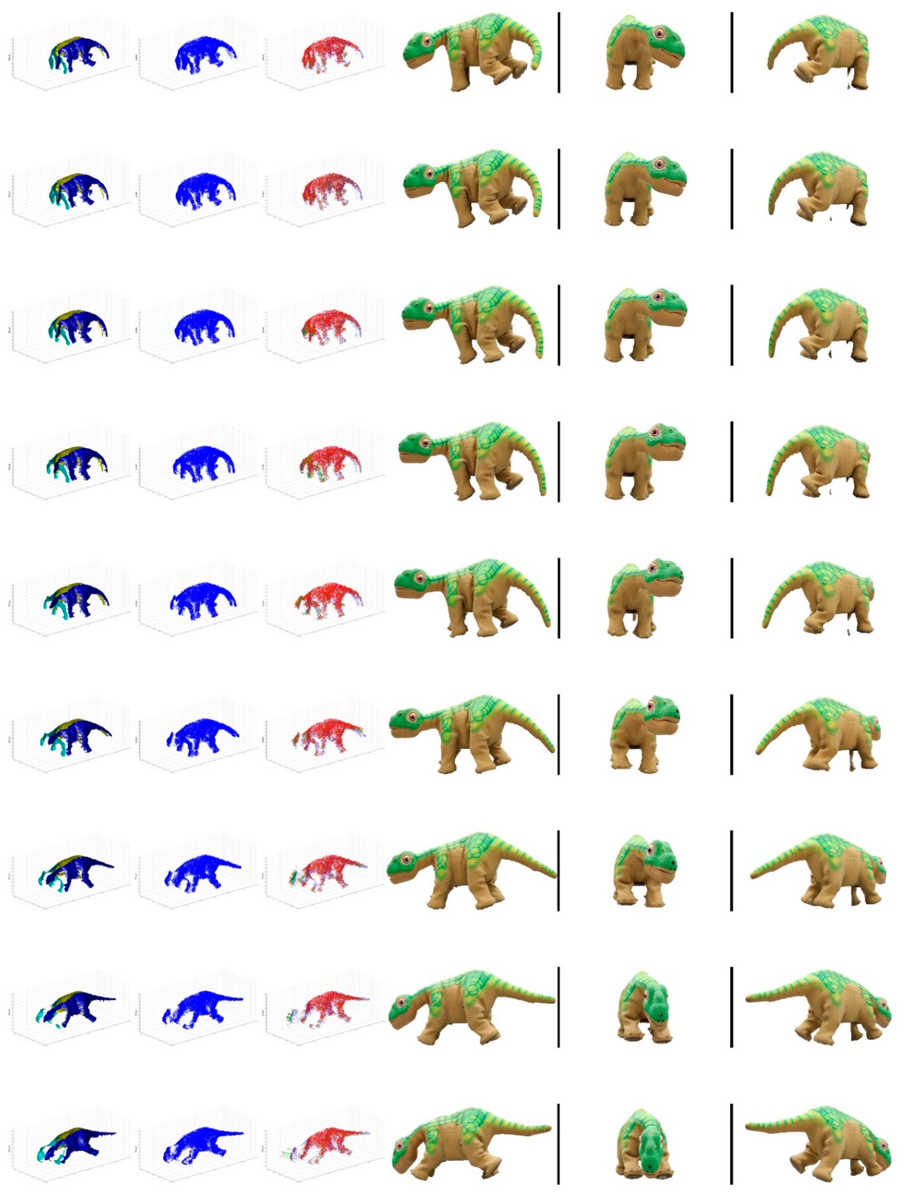
The following figure illustrates a movie-strip representation of the captured data from the experiments. The left-most column represents the predicted deformation of surface patches, the second column represents the recovered point cloud at the demand instant, and the third column represents the tracking to prediction offsets, while the last three columns represent the viewpoint from one camera from each stereo pair.
Figure A3.
Unoccluded Experiment 1 movie-strip.

References
- Olague, G.; Mohr, R. Optimal camera placement for accurate reconstruction. Pattern Recognit. 2002, 35, 927–944. [Google Scholar] [CrossRef] [Green Version]
- MacKay, M.D.; Fenton, R.G.; Benhabib, B. Multi-camera active surveillance of an articulated human form—An implementation strategy. Comput. Vis. Image Underst. 2011, 115, 1395–1413. [Google Scholar] [CrossRef]
- Schacter, D.S.; Donnici, M.; Nuger, E.; MacKay, M.D.; Benhabib, B. A multi-camera active-vision system for deformable-object-motion capture. J. Intell. Robot. Syst. 2014, 75, 413–441. [Google Scholar] [CrossRef]
- Furukawa, Y.; Ponce, J. Accurate, dense, and robust multiview stereopsis. IEEE Trans. Pattern Anal. Mach. Intell. 2010, 32, 1362–1376. [Google Scholar] [CrossRef] [PubMed]
- Koch, A.; Dipanda, A. Direct 3D Information Determination in an Uncalibrated Stereovision System by Using Evolutionary Algorithms. Intell. Comput. Vis. Image Process. Innov. Appl. Des. Innov. Appl. Des. 2013, 101. [Google Scholar] [CrossRef]
- Forsyth, D.A.; Ponce, J. Computer Vision: A Modern Approach, 2nd ed.; Pearson: London, UK, 2012. [Google Scholar]
- Blais, F. Review of 20 years of range sensor development. J. Electron. Imaging 2004, 13, 231–240. [Google Scholar] [CrossRef]
- Slembrouck, M.; Niño-Castañeda, J.; Allebosch, G.; van Cauwelaert, D.; Veelaert, P.; Philips, W. High performance multi-camera tracking using shapes-from-silhouettes and occlusion removal. In Proceedings of the 9th International Conference on Distributed Smart Camera, Seville, Spain, 8–11 September 2015; pp. 44–49. [Google Scholar]
- Goesele, M.; Curless, B.; Seitz, S.M. Multi-view stereo revisited. In Proceedings of the IEEE Computer Society Conference on Computer Vision and Pattern Recognition, New York, NY, USA, 17–22 June 2006; Volume 2, pp. 2402–2409. [Google Scholar]
- de Aguiar, E.; Stoll, C.; Theobalt, C.; Ahmed, N.; Seidel, H.-P.; Thrun, S. Performance Capture from Sparse Multi-View Video. ACM Trans. Graph. 2008, 27, 98–108. [Google Scholar] [CrossRef]
- McNeil, J.G.; Lattimer, B.Y. Real-Time Classification of Water Spray and Leaks for Robotic Firefighting. Int. J. Comput. Vis. Image Process. 2015, 5, 1–26. [Google Scholar] [CrossRef]
- Lee, K.-R.; Nguyen, T. Realistic surface geometry reconstruction using a hand-held RGB-D camera. Mach. Vis. Appl. 2016, 27, 377–385. [Google Scholar] [CrossRef]
- MacKay, M.D.; Fenton, R.G.; Benhabib, B. Time-varying-geometry object surveillance using a multi-camera active-vision system. Int. J. Smart Sens. Intell. Syst. 2008, 1, 679–704. [Google Scholar] [CrossRef]
- Schacter, D.S. Multi-Camera Active-Vision System Reconfiguration for Deformable Object Motion Capture; University of Toronto: Toronto, ON, Canada, 2014. [Google Scholar]
- Gupta, J.P.; Singh, N.; Dixit, P.; Semwal, V.B.; Dubey, S.R. Human activity recognition using gait pattern. Int. J. Comput. Vis. Image Process. 2013, 3, 31–53. [Google Scholar] [CrossRef]
- Kulikova, M.; Jermyn, I.; Descombes, X.; Zhizhina, E.; Zerubia, J. A marked point process model including strong prior shape information applied to multiple object extraction from images. Intell. Comput. Vis. Image Process. Innov. Appl. Des. Innov. Appl. Des. 2013, 71. [Google Scholar] [CrossRef]
- Naish, M.D.; Croft, E.A.; Benhabib, B. Simulation-based sensing-system configuration for dynamic dispatching. In Proceedings of the IEEE International Conference on Systems, Man and Cybernetics, Tucson, AZ, USA, 7–10 October 2001; Volume 5, pp. 2964–2969. [Google Scholar]
- Zhang, Z.; Xu, D.; Yu, J. Research and Latest Development of Ping-Pong Robot Player. In Proceedings of the 7th World Congress on Intelligent Control. and Automation, Chongqing, China, 25–27 June 2008; pp. 4881–4886. [Google Scholar]
- Barteit, D.; Frank, H.; Kupzog, F. Accurate Prediction of Interception Positions for Catching Thrown Objects in Production Systems. In Proceedings of the 6th IEEE International Conference on Industrial Informatics, Daejeon, Korea, 13–16 July 2008; pp. 893–898. [Google Scholar]
- Tomasi, C.; Kanade, T. Shape and motion from image streams: A factorization method. Proc. Natl. Acad. Sci. USA 1993, 90, 9795–9802. [Google Scholar] [CrossRef] [PubMed]
- Pollefeys, M.; Vergauwen, M.; Cornelis, K.; Tops, J.; Verbiest, F.; van Gool, L. Structure and motion from image sequences. In Proceedings of the Conference on Optical 3D Measurement Techniques, Zurich, Switzerland, 22–25 September 2001; pp. 251–258. [Google Scholar]
- Lhuillier, M.; Quan, L. A quasi-dense approach to surface reconstruction from uncalibrated images. IEEE Trans. Pattern Anal. Mach. Intell. 2005, 27, 418–433. [Google Scholar] [CrossRef] [PubMed] [Green Version]
- Snavely, N.; Seitz, S.M.; Szeliski, R. Photo tourism: Exploring photo collections in 3D. ACM Trans. Graph. 2006, 25, 835–846. [Google Scholar] [CrossRef]
- Jin, H.; Soatto, S.; Yezzi, A.J. Multi-view stereo reconstruction of dense shape and complex appearance. Int. J. Comput. Vis. 2005, 63, 175–189. [Google Scholar] [CrossRef]
- Jancosek, M.; Pajdla, T. Multi-view reconstruction preserving weakly-supported surfaces. In Proceedings of the IEEE Conference on Computer Vision and Pattern Recognition, Colorado Springs, CO, USA, 20–25 June 2011; pp. 3121–3128. [Google Scholar]
- Furukawa, Y.; Ponce, J. Carved visual hulls for image-based modeling. In Proceedings of the European Conference on Computer Vision, Graz, Austria, 7–13 May 2006; pp. 564–577. [Google Scholar]
- Li, Q.; Xu, S.; Xia, D.; Li, D. A novel 3D convex surface reconstruction method based on visual hull. Pattern Recognit. Comput. Vis. 2011, 8004, 800412. [Google Scholar]
- Roshnara Nasrin, P.P.; Jabbar, S. Efficient 3D visual hull reconstruction based on marching cube algorithm. In Proceedings of the International Conference on Innovations in Information, Embedded and Communication Systems (ICIIECS), Coimbatore, India, 19–20 March 2015; pp. 1–6. [Google Scholar]
- Laurentini, A. Visual hull concept for silhouette-based image understanding. IEEE Trans. Pattern Anal. Mach. Intell. 1994, 16, 150–162. [Google Scholar] [CrossRef]
- Esteban, C.H.; Schmitt, F. Silhouette and stereo fusion for 3d object modeling. Comput. Vis. Image Underst. 2004, 96, 367–392. [Google Scholar] [CrossRef]
- Terauchi, T.; Oue, Y.; Fujimura, K. A flexible 3D modeling system based on combining shape-from-silhouette with light-sectioning algorithm. In Proceedings of the International Conference on 3-D Digital Imaging and Modeling, San Diego, CA, USA, 20–25 June 2005; pp. 196–203. [Google Scholar]
- Yemez, Y.; Wetherilt, C.J. A volumetric fusion technique for surface reconstruction from silhouettes and range data. Comput. Vis. Image Underst. 2007, 105, 30–41. [Google Scholar] [CrossRef]
- Cremers, D.; Kolev, K. Multiview stereo and silhouette consistency via convex functionals over convex domains. IEEE Trans. Pattern Anal. Mach. Intell. 2011, 33, 1161–1174. [Google Scholar] [CrossRef] [PubMed]
- Guan, L.; Franco, J.-S.; Pollefeys, M. Multi-Object Shape Estimation and Tracking from Silhouette Cues. In Proceedings of the IEEE Conference on Computer Vision and Pattern Recognition, Anchorage, AK, USA, 23–28 June 2008; pp. 1–8. [Google Scholar]
- Sedai, S.; Bennamoun, M.; Huynh, D.Q. A Gaussian Process Guided Particle Filter For Tracking 3D Human Pose In Video. IEEE Trans. Image Process. 2013, 22, 4286–4300. [Google Scholar] [CrossRef] [PubMed]
- Lallemand, J.; Szczot, M.; Ilic, S. Human Pose Estimation in Stereo Images. In Proceedings of the 8th International Conference on Articulated Motion and Deformable Objects, Palma de Mallorca, Spain, 16–18 July 2014; pp. 10–19. [Google Scholar]
- Charles, J.; Pfister, T.; Everingham, M.; Zisserman, A. Automatic and Efficient Human Pose Estimation for Sign Language Videos. Int. J. Comput. Vis. 2014, 110, 70–90. [Google Scholar] [CrossRef]
- López-Quintero, M.I.; Marin-Jiménez, M.J.; Muñoz-Salinas, R.; Madrid-Cuevas, F.J.; Medina-Carnicer, R. Stereo Pictorial Structure for 2D articulated human pose estimation. Mach. Vis. Appl. 2016, 27, 157–174. [Google Scholar] [CrossRef]
- Biasi, N.; Setti, F. Garment-based motion capture (GaMoCap): High-density capture of human shape in motion. Mach. Vis. Appl. 2015, 26, 955–973. [Google Scholar] [CrossRef]
- Hasler, N.; Rosenhahn, B.; Thormählen, T.; Wand, M.; Gall, J.; Seidel, H.P. Markerless motion capture with unsynchronized moving cameras. In Proceedings of the IEEE Conference on Computer Vision and Pattern Recognition (CVPR), Miami, FL, USA, 20–25 June 2009; pp. 224–231. [Google Scholar]
- Bradley, D.; Popa, T.; Sheffer, A.; Heidrich, W.; Boubekeur, T. Markerless garment capture. ACM Trans. Graph. 2008, 27, 1–9. [Google Scholar] [CrossRef]
- Bradley, D.; Heidrich, W.; Popa, T.; Sheffer, A. High Resolution Passive Facial Performance Capture. ACM Trans. Graph. 2010, 29, 41–50. [Google Scholar] [CrossRef]
- Corazza, S.; Mündermann, L.; Gambaretto, E.; Ferrigno, G.; Andriacchi, T.P. Markerless motion capture through visual hull, articulated ICP and subject specific model generation. Int. J. Comput. Vis. 2010, 87, 156–169. [Google Scholar] [CrossRef]
- Corazza, S.; Muendermann, L.; Chaudhari, A.M.; Demattio, T.; Cobelli, C.; Andriacchi, T.P. A markerless motion capture system to study musculoskeletal biomechanics: Visual hull and simulated annealing approach. Ann. Biomed. Eng. 2006, 34, 1019–1029. [Google Scholar] [CrossRef] [PubMed]
- Schulman, J.; Lee, A.; Ho, J.; Abbeel, P. Tracking Deformable Objects with Point Clouds. In Proceedings of the IEEE International Conference on Robotics and Automation, Karlsruhe, Germany, 6–10 May 2013; pp. 1130–1137. [Google Scholar]
- Petit, B.; Lesage, J.D. Multicamera real-time 3D modeling for telepresence and remote collaboration. Int. J. Digit. Multimed. Broadcast. 2010, 2010. [Google Scholar] [CrossRef]
- Matsuyama, T.; Wu, X.; Takai, T.; Nobuhara, S. Real-time 3D shape reconstruction, dynamic 3D mesh deformation, and high delity visualization for 3D video. Comput. Vis. Image Underst. 2004, 96, 393–434. [Google Scholar] [CrossRef]
- Hapák, J.; Jankó, Z.; Chetverikov, D. Real-Time 4D Reconstruction of Human Motion. In Proceedings of the 7th International Conference on Articulated Motion and Deformable Objects, Mallorca, Spain, 11–13 July 2012; pp. 250–259. [Google Scholar]
- Tsekourakis, I.; Mordohai, P. Consistent 3D Background Model Estimation from Multi-viewpoint Videos. In Proceedings of the International Conference on 3D Vision (3DV), Lyon, France, 19–22 October 2015; pp. 144–152. [Google Scholar]
- Kalman, R.E. A New Approach to Linear Filtering and Prediction Problems 1. ASME Trans. J. Basic Eng. 1960, 82, 35–45. [Google Scholar] [CrossRef]
- Naish, M.D.; Croft, E.A.; Benhabib, B. Coordinated dispatching of proximity sensors for the surveillance of manoeuvring targets. Robot. Comput. Integr. Manuf. 2003, 19, 283–299. [Google Scholar] [CrossRef]
- Bakhtari, A.; Naish, M.D.; Eskandari, M.; Croft, E.A.; Benhabib, B. Active-vision-based multisensor surveillance-an implementation. IEEE Trans. Syst. Man Cybern. Part C Appl. Rev. 2006, 36, 668–680. [Google Scholar] [CrossRef]
- Bakhtari, A.; MacKay, M.D.; Benhabib, B. Active-vision for the autonomous surveillance of dynamic, multi-object environments. J. Intell. Robot. Syst. 2009, 54, 567–593. [Google Scholar] [CrossRef]
- Ristic, B.; Arulampalam, S.; Gordon, N. A tutorial on particle filters. In Beyond the Kalman Filter: Particle Filter for Tracking Applications; Artech House: Boston, MA, USA, 2004; pp. 35–62. [Google Scholar]
- Eberhart, R.C.; Kennedy, J. A new optimizer using particle swarm theory. In Proceedings of the Sixth International Symposium on Micro Machine and Human, Nagoya, Japan, 4–6 October 1995; Volume 1, pp. 39–43. [Google Scholar]
- Zhang, X. A swarm intelligence based searching strategy for articulated 3D human body tracking. In Proceedings of the IEEE Conference on Computer Vision and Pattern Recognition, San Francisco, CA, USA, 13–18 June 2010; pp. 45–50. [Google Scholar]
- Kwolek, B.; Krzeszowski, T.; Gagalowicz, A.; Wojciechowski, K.; Josinski, H. Real-time multi-view human motion tracking using particle swarm optimization with resampling. In Proceedings of the International Conference on Articulated Motion and Deformable Objects (AMDO), Mallorca, Spain, 11–13 July 2012; pp. 92–101. [Google Scholar]
- Richa, R.; Bó, A.P.L.; Poignet, P. Towards Robust 3D Visual Tracking for Motion Compensation in Beating Heart Surgery. Med. Image Anal. 2011, 15, 302–315. [Google Scholar] [CrossRef] [PubMed]
- Popham, T. Tracking 3D Surfaces Using Multiple Cameras: A Probabilistic Approach; University of Warwick: Coventry, UK, 2010. [Google Scholar]
- Furukawa, Y.; Ponce, J. Dense 3D motion capture for human faces. In Proceedings of the IEEE Conference on Computer Vision and Pattern Recognition, Miami, FL, USA, 10–25 June 2009; pp. 1674–1681. [Google Scholar]
- Hernández-Rodriguez, F.; Castelán, M. A photometric sampling method for facial shape recovery. Mach. Vis. Appl. 2016, 27, 483–497. [Google Scholar] [CrossRef]
- Lowe, D.G. Object Recognition from Local Scale-Invariant Features. In Proceedings of the 7th IEEE International Conference on Computer Vision, Kerkyra, Greece, 20–27 September 1999; Volume 2, pp. 1150–1157. [Google Scholar]
- Lowe, D.G. Distinctive image features from scale-invariant keypoints. Int. J. Comput. Vis. 2004, 60, 91–110. [Google Scholar] [CrossRef]
- Yu, G.; Morel, J.-M. ASIFT: An Algorithm for Fully Affine Invariant Comparison. Image Process. Line 2011, 1, 11–38. [Google Scholar] [CrossRef]
- Bay, H.; Ess, A.; Tuytelaars, T.; van Gool, L. Speeded up robust features (SURF). Comput. Vis. Image Underst. 2008, 110, 346–359. [Google Scholar] [CrossRef]
- Doshi, A.; Starck, J.; Hilton, A. An Empirical Study of Non-Rigid Surface Feature Matching of Human from 3D Video. J. Virtual Real. Broadcast. 2010, 7, 1860–2037. [Google Scholar]
- Khan, N.; McCane, B.; Mills, S. Better than SIFT? Mach. Vis. Appl. 2015, 26, 819–836. [Google Scholar] [CrossRef]
- Brown, M.; Lowe, D.G. Automatic panoramic image stitching using invariant features. Int. J. Comput. Vis. 2007, 74, 59–73. [Google Scholar] [CrossRef]
- Du, X.; Tan, K.K. Vision-based approach towards lane line detection and vehicle localization. Mach. Vis. Appl. 2016, 27, 175–191. [Google Scholar] [CrossRef]
- Altuntas, C. Pair-wise automatic registration of three-dimensional laser scanning data from historical building by created two-dimensional images. Opt. Eng. 2014, 53, 53108. [Google Scholar] [CrossRef]
- Moisan, L.; Stival, B. A probabilistic criterion to detect rigid point matches between two images and estimate the fundamental matrix. Int. J. Comput. Vis. 2004, 57, 201–218. [Google Scholar] [CrossRef]
- Owczarek, M.; Baranski, P.; Strumillo, P. Pedestrian tracking in video sequences: A particle filtering approach. In Proceedings of the Federated Conference on Computer Science and Information Systems, Lodz, Poland, 13–16 September 2015; pp. 875–881. [Google Scholar]
- Welch, G.; Bishop, G. An introduction to the Kalman filter. In Pract. 2006, 7, 1–16. [Google Scholar]
- Chen, S.Y. Kalman filter for robot vision: A survey. IEEE Trans. Ind. Electron. 2012, 59, 4409–4420. [Google Scholar] [CrossRef]
- Marron, M.; Garcia, J.C.; Sotelo, M.A.; Cabello, M.; Pizarro, D.; Huerta, F.; Cerro, J. Comparing a Kalman Filter and a Particle Filter in a Multiple Objects Tracking Application. In Proceedings of the IEEE International Symposium on Intelligent Signal Processing, Alcala de Henares, Spain, 3–5 October 2007; pp. 1–6. [Google Scholar]
- Chen, S.; Li, Y.; Kwok, N.M. Active vision in robotic systems: A survey of recent developments. Int. J. Rob. Res. 2011, 30, 1343–1377. [Google Scholar] [CrossRef]
- Leizea, I.; Álvarez, H.; Borro, D. Real time non-rigid 3D surface tracking using particle filter. Comput. Vis. Image Underst. 2015, 133, 51–65. [Google Scholar] [CrossRef]
- Hasinoff, S.W.; Durand, F.; Freeman, W.T. Noise-optimal capture for high dynamic range photography. In Proceedings of the IEEE Conference on Computer Vision and Pattern Recognition, San Francisco, CA, USA, 13–18 June 2010; pp. 553–560. [Google Scholar]
- Richa, R.; Poignet, P. Efficient 3D Tracking for Motion Compensation in Beating Heart Surgery. Int. Conf. Med. Image Comput. Comput. Interv. 2008, 11, 684–691. [Google Scholar]
- Blender Online Community Blender—A 3D Modelling and Rendering Package; Blender Institute: Amsterdam, The Netherlands, 2016.
- Vedaldi, A.; Fulkerson, B. {VLFeat}—An open and portable library of computer vision algorithms. In Proceedings of the ACM International Conference on Multimedia, Firenze, Italy, 25–29 October 2010. [Google Scholar]
- Li, X.; Zhu, S.; Chen, L. Statistical background model-based target detection. Pattern Anal. Appl. 2016, 19, 783–791. [Google Scholar] [CrossRef]
- Nieto, M.; Ortega, J.D.; Leškovský, P.; Senderos, O. Constant-time monocular object detection using scene geometry. Pattern Anal. Appl. 2018, 21, 1053–1066. [Google Scholar] [CrossRef]
- Mignotte, M. A biologically inspired framework for contour detection. Pattern Anal. Appl. 2017, 20, 365–381. [Google Scholar] [CrossRef]
- Ye, S.; Liu, C.; Li, Z. A double circle structure descriptor and Hough voting matching for real-time object detection. Pattern Anal. Appl. 2016, 19, 1143–1157. [Google Scholar] [CrossRef]
- Tang, M.; Gorelick, L.; Veksler, O.; Boykov, Y. Grabcut in one cut. In Proceedings of the 2013 IEEE International Conference on Computer Vision (ICCV), Sydney, Australia, 1–8 December 2013; pp. 1769–1776. [Google Scholar]
Figure 1.
Proposed methodology.

Figure 2.
Triangulated surface patches from each stereo-camera pair, units in [mm].

Figure 3.
Proposed shape-prediction algorithm.

Figure 4.
Movie-strip of Simulation 1, units in [mm].

Figure 5.
Left: triangulation, prediction, and relative prediction error metrics for each demand instant. Right: total number of tracked and triangulated points for each demand instant.
Figure 5.
Left: triangulation, prediction, and relative prediction error metrics for each demand instant. Right: total number of tracked and triangulated points for each demand instant.

Figure 6.
Movie-strip of Simulation 2, units in [mm].

Figure 7.
Left: triangulation, prediction, and relative prediction error metrics for each demand instant. Right: total number of tracked and triangulated points for each demand instant.
Figure 7.
Left: triangulation, prediction, and relative prediction error metrics for each demand instant. Right: total number of tracked and triangulated points for each demand instant.

Figure 8.
Movie-strip of Simulation 3, units in [mm].

Figure 9.
Left: triangulation, prediction, and relative prediction error metrics for each demand instant. Right: total number of tracked and triangulated points for each demand instant.
Figure 9.
Left: triangulation, prediction, and relative prediction error metrics for each demand instant. Right: total number of tracked and triangulated points for each demand instant.

Figure 10.
Experimental set-up.

Figure 11.
Stereo-camera simulation process for one demand instant, (a) first camera position, (b) second camera position. Units in [mm].
Figure 11.
Stereo-camera simulation process for one demand instant, (a) first camera position, (b) second camera position. Units in [mm].

Figure 12.
PLEOrb robot properties.

Figure 13.
Background segmentation through GrabCut: (a) input image with guides; (b) resulting binary segmented image.
Figure 13.
Background segmentation through GrabCut: (a) input image with guides; (b) resulting binary segmented image.

Figure 14.
Unoccluded Experiment 1.

Figure 15.
Unoccluded Experiment 2.

Figure 16.
Unoccluded Experiment 3.

Figure 17.
Unoccluded Experiment 4.

Figure 18.
Unoccluded Experiment 5.

Figure 19.
Occluded Experiment 1.

Figure 20.
Occluded Experiment 2.

Figure 21.
Occluded Experiment 3.

Figure 22.
Occluded Experiment 4.

Figure 23.
Occluded Experiment 5.


Table 1.
Average processing time for experiments.
| Experiment | Unoccluded | Occluded |
|---|---|---|
| 1 | 25.58 s | 26.61 s |
| 2 | 24.78 s | 25.57 s |
| 3 | 31.10 s | 32.92 s |
| 4 | 19.48 s | 24.73 s |
| 5 | 20.51 s | 23.24 s |
© 2018 by the authors. Licensee MDPI, Basel, Switzerland. This article is an open access article distributed under the terms and conditions of the Creative Commons Attribution (CC BY) license (http://creativecommons.org/licenses/by/4.0/).
Share and Cite
MDPI and ACS Style
Nuger, E.; Benhabib, B. A Methodology for Multi-Camera Surface-Shape Estimation of Deformable Unknown Objects. Robotics 2018, 7, 69. https://doi.org/10.3390/robotics7040069
AMA Style
Nuger E, Benhabib B. A Methodology for Multi-Camera Surface-Shape Estimation of Deformable Unknown Objects. Robotics. 2018; 7(4):69. https://doi.org/10.3390/robotics7040069
Chicago/Turabian StyleNuger, Evgeny, and Beno Benhabib. 2018. "A Methodology for Multi-Camera Surface-Shape Estimation of Deformable Unknown Objects" Robotics 7, no. 4: 69. https://doi.org/10.3390/robotics7040069
Note that from the first issue of 2016, this journal uses article numbers instead of page numbers. See further details here.