Hitchhiking Based Symbiotic Multi-Robot Navigation in Sensor Networks
by
 , , ,
, , ,
Abhijeet Ravankar
1,*,† ,
,
Ankit A. Ravankar
2,†,
Yukinori Kobayashi
2,
Yohei Hoshino
1,
Chao-Chung Peng
3 and
Michiko Watanabe
1 1
School of Regional Innovation and Social Design Engineering, Faculty of Engineering, Kitami Institute of Technology, Kitami, Hokkaido 090-8507, Japan
2
Division of Human Mechanical Systems and Design, Faculty of Engg., Hokkaido University, Sapporo, Hokkaido 060-8628, Japan
3
Department of Aeronautics and Astronautics, National Cheng Kung University, Tainan 701, Taiwan
*
Author to whom correspondence should be addressed.
†
These authors contributed equally to this work.
Robotics 2018, 7(3), 37; https://doi.org/10.3390/robotics7030037
Submission received: 24 May 2018
/
Revised: 20 June 2018
/
Accepted: 12 July 2018
/
Published: 15 July 2018
(This article belongs to the Special Issue Distributed, Ubiquitous and Multi-Agent Robotic Architectures)
Abstract
:Robot navigation is a complex process that involves real-time localization, obstacle avoidance, map update, control, and path planning. Thus, it is also a computationally expensive process, especially in multi-robot systems. This paper presents a cooperative multi-robot navigation scheme in which a robot can ‘hitchhike’ another robot, i.e., two robots going to the same (or close) destination navigate together in a leader–follower system assisted by visual servoing. Although such cooperative navigation has many benefits compared to traditional approaches with separate navigation, there are many constraints to implementing such a system. A sensor network removes those constraints by enabling multiple robots to communicate with each other to exchange meaningful information such as their respective positions, goal and destination locations, and drastically improves the efficiency of symbiotic multi-robot navigation through hitchhiking. We show that the proposed system enables efficient navigation of multi-robots without loss of information in a sensor network. Efficiency improvements in terms of reduced waiting time of the hitchhiker, not missing potential drivers, best driver-profile match, and velocity tuning are discussed. Novel algorithms for partial hitchhiking, and multi-driver hitchhiking are proposed. A novel case of hitchhiking based simultaneous multi-robot teleoperation by a single operation is also proposed. All the proposed algorithms are verified by experiments in both simulation and real environment.
1. Introduction
With recent advances in artificial intelligence and sensor technologies, it is anticipated that more and more robots will be used for several services like cleaning, patrolling, and moving items at home and public places. Using multiple robots has several benefits compared to using a single robot for such tasks. A multi-robot system enables task parallelism, fault tolerance, and diverse execution of tasks at the same time. Consider an item delivery multi-robot system in a large and complex environment in which the goal locations of the robots vary from time to time. In such a multi-robot system, each robot has to navigate to different locations in the map to provide its designated services (deliver items). In order to do this, mobile robots are equipped with a navigation module that depends on other modules. For example, a robot must have the map of the environment with obstacles marked in it that is provided by the mapping module. Similarly, robots need to localize and simultaneously update the new obstacles in the map provided by the Simultaneous Localization and Mapping [1] (SLAM) module. Then, there is the control module to steer the robot properly towards the goal without hitting the obstacles that could be static or dynamic (like moving people in corridors) on the planned path.
Thus, robot navigation is a complex process and depends on a lot of modules, most of which are computationally expensive. For example, 3D SLAM module for 3D localization and mapping using RGBD (RGB color and Depth) sensors requires processing of a lot of data and is computationally expensive. In the context of multi-robot systems, each robot must execute all these computationally expensive modules by itself. Since most of the robots are battery operated, executing these modules consumes battery power, which decreases the service time of these robots, and they require frequent recharging.
However, if two (or more) robots have the same start and goal locations, then separately executing path planning, localization, mapping, and obstacle avoidance modules is a waste of computation (and hence battery power). Instead, a robot can ‘hitchhike’ another robot going to the same goal and save its computation by merely following it. We presented this idea in our previous work [2], in which a ‘hitchhiking’ robot initiates a request and attaches itself behind a ‘driver’ robot going to the same location by using visual servoing. The hitchhiking robot shuts down all of its modules except visual servoing, and completely relies on the driver robot to navigate, thus saving computation. This approach is different from the traditional leader–follower system that has been proposed earlier for a different set of objectives. For example, in order to coordinate agriculture tasks in fields, a system of two tractors has been proposed [3,4] to improve efficiency in agricultural tasks in which the focus is on cooperation and coordination to execute a turn without collision. Similarly, cooperative localization and mapping has also been proposed [5,6,7,8]. Works in [9,10,11] discuss multi-robot navigation. An effort to ease teleoperation is proposed in [12], which uses leader–follower robots in master–slave configuration. Work in [13] considers applications where a human agent is navigating a semi-autonomous mobile robot in an environment with obstacles. A group of wheeled robots with nonholonomic constraints is considered to rendezvous at a specific point with a desired orientation while maintaining network connectivity and ensuring collision avoidance within the robots in [14]. A bio-inspired approach for multi-robot exploration has also been proposed in [15]. Various algorithms for multi-robot path planning have also been proposed. Multi-robot path planning can be centralized [16] or decentralized [17]. Multi-robot collision avoidance has been discussed in [18].
Most of the previously proposed leader–follower multi-robot systems have different objectives. However, the proposed hitchhiking mechanism aims at cooperative navigation towards the common goal location, in which the hitchhiking robot shuts down all of its modules except visual servoing and completely relies on the driver robot for navigation. Moreover, the driver makes sure that the hitchhiker does not lose any information (like new obstacle positions). For multi-robot scenarios, the only requirement of the system is networking between the different robots, and a sensor network provides such capabilities. Moreover, the proposed architecture allows the robots to benefit from the sensor network [19] in the infrastructure.
This work is an extension of our previous work [2]. The previously proposed work had several constraints and drawbacks in terms of waiting time, coupling, and profile confirmation. Inability of long-range communication between the robots, and local-only communication were the major bottlenecks that resulted in those constraints. Hence, we extend and improve the previous work by considering robots in a sensor network in which the aforementioned problems are resolved by intelligent and timely information exchange between the robots. For the benefit of new readers, we first briefly introduce multi-robot hitchhiking. We then explain its limitations, and how those limitations can be solved in a sensor network. The present work discusses novel algorithms and modes of hitchhiking in a sensor network and its advantages.
The new contributions of this work are summarized below:
- The present work discusses novel algorithms for hitchhiking in sensor networks that enable long-range communication between robots. The advantages in terms of reduced waiting time of the hitchhiker, not missing potential drivers, best driver-profile match, and velocity tuning are discussed.
- A novel mode of ‘partial hitchhiking’ is presented in which hitchhiking is executed only for a partial portion of the path.
- A novel mode of ‘multi-driver hitchhiking’ is proposed in which a hitchhiker uses multiple driver robots to navigate to its goal location.
- A novel usage of hitchhiking for simultaneous teleoperation of multiple robots by a single operator is presented and its advantages are discussed.
2. A Brief Overview of Hitchhiking Robots
An actual implementation of hitchhiking in real robots requires fusing the various steps of hitchhiking (Figure 1b) directly into the SLAM module. Our previous work [2] discusses the mathematical details of fusing the hitchhiking steps in an Extended Kalman Filter (EKF) based SLAM. This section provides a very brief introduction of hitchhiking in multi-robot systems.
2.1. System Configuration
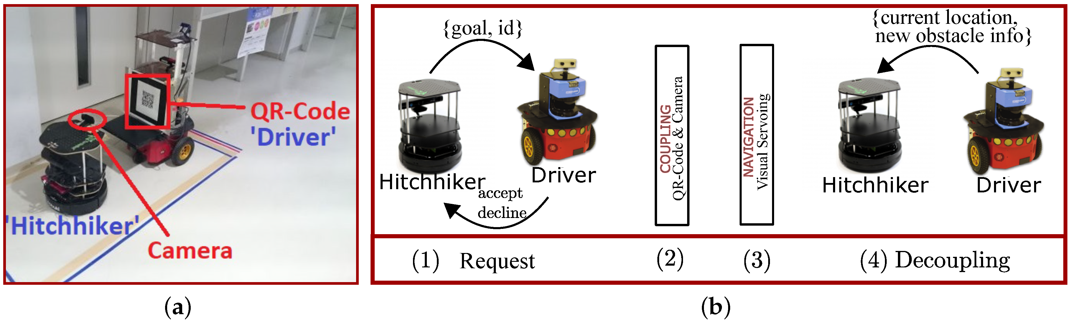
Figure 1a shows the hitchhiking setup. It is comprised of robots that are equipped with front facing cameras and QR-code markers to assist with visual servoing. Although QR-codes are not necessary, an easy to detect pattern helps in robust visual servoing. The leader robot in front is called a ‘Driver’ robot, whereas the follower robot is termed a ‘Hitchhiker’ robot. It is assumed that the robots are in a sensor network and have networking capabilities to communicate with each other. Each robot is assigned an ID (). Robots could have a different set of sensors attached to them. Based on the accuracy, range of sensors, and accuracy of navigation and its dependent modules, each robot is also given a profile score (). Higher scores indicate a better set of sensors and navigation modules. The profile score is set manually for each robot and is a static value, as generally the attached sensors and navigation software of a robot does not change. A priority is associated with each task assigned to the robot. Priority is a numerical value in range 0 to 20, and higher values signify high priority and vice-versa. If a robot is not assigned a priority, a default value of 10 is used. A user can assign high priorities to time critical tasks that must be finished quickly. Hitchhiking is denied (for both driver and hitchhiker) in a task priority range of 16 to 20.
The hitchhiker robot follows the driver robot through visual servoing. A complete description of visual servoing is not in the scope of the present work and a simple explanation is provided. Visual servoing [20] is the motion control of a robot using feedback information from a camera. It works by extracting visual features from the QR-code markers, and a set of visual measurements that are coordinates of points of interest, i.e., . A controller then minimizes the error vector , so that the features reach a desired value . The required trajectory is generated and details can be found in [21,22].
2.2. Flow of Hitchhiking Process
Hitchhiking is carried out in four steps shown in Figure 1b and described below:
- Hitchhiking Request: The process of hitchhiking starts with a request from a hitchhiker. The hitchhiker broadcast a request which is comprised of : Robot-ID, : Goal Location, and : Robot profile}. A potential driver accepts or rejects the request depending on whether: (a) it is going to the same (or close) location, and (b) its profile score is greater than or equal to the hitchhiker’s profile score. The later check of the profile score ensures that the driver is a robot with better sensor specifications and navigation module than the hitchhiker.
- Coupling: Once a potential driver robot going to the same goal location accepts the request, the two robots ‘couple’ in a configuration shown in Figure 1a using a camera and QR-code. Artificial markers can be laid in the environment to assist coupling.
- Navigation: The driver robot starts navigation and the hitchhiker starts following the driver using visual servoing. During navigation, the hitchhiker only executes visual servoing and shuts down the other modules of localization, path planning, obstacle avoidance, and map update modules.
- Decoupling: Upon reaching the goal, the driver robot transfers the current pose, and new static obstacles found in the way to the hitchhiker and the hitchhiking terminates. An example of a driver’s message is given in Listing 1.
The hitchhiker can thus skip redundant computation from the hitchhiking point to the decoupling location without any information loss (e.g., location of new static obstacles in the path). However, there are several drawbacks of implementing hitchhiking in the absence of a sensor network. These limitations are explained below.
Recovery from ‘Driver Lost’ Scenario
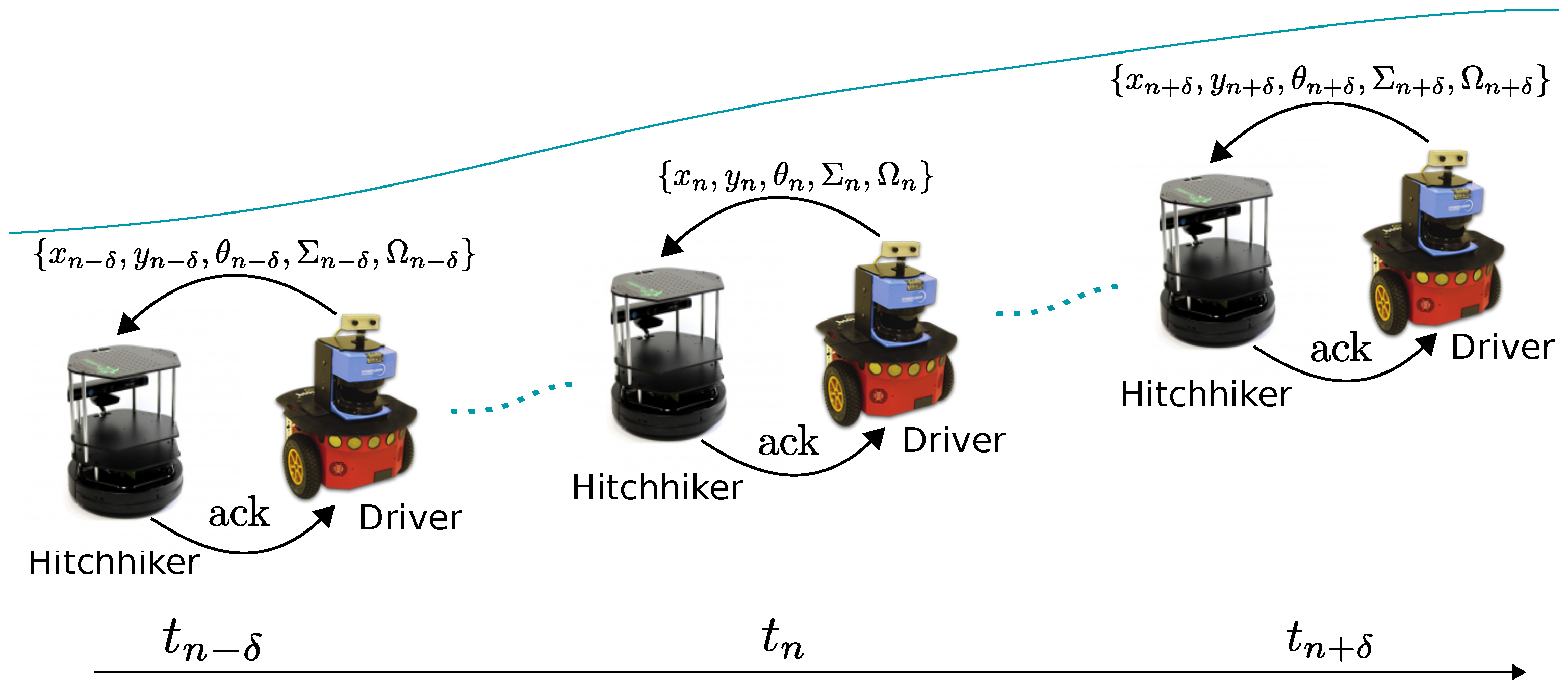
Visual servoing is not the only method of following the driver robot by the hitchhiker and other robust methods can be employed. In the context of the proposed work, robustness of hitchhiking depends on the robustness of visual servoing. Visual servoing is not very robust to large rotations, and the driver might be ‘lost’ by the hitchhiker during navigation. In other words, the follower robot will be left behind while the driver robot navigates to its goal. Work by Francois [23] has provided details of the problems in visual servoing and any of the reasons might result in a driver lost scenario.
The hitchhiker only executes a visual servoing module to follow the driver. Hence, if the driver is lost, then it will be difficult for the hitchhiker to localize itself in the map as it is completely unaware of its current position in the map. This problem is similar to the famous ‘kidnapped robot problem’ for which solutions are available in literature [24,25,26]. However, we propose to recover from this problem in the first place by transferring the current estimated pose () and associated uncertainty () information to the hitchhiker intermittently in intervals of s. This is graphically shown in Figure 2 where a driver is shown transferring information intermittently. With this scheme, even if the driver robot is lost due to failure of visual servoing, the hitchhiker still has a rough initial estimate to localize itself in the map, and navigate towards the goal independently. Moreover, the hitchhiker also acknowledges receiving the intermittent data from the driver. If the driver does not receive the acknowledgement message (ack) from the hitchhiker, then it stops for the hitchhiker to catch up. In general, visual servoing is good enough provided the driver navigates at a slow speed and avoids sudden sharp turns.
3. Limitations of Hitchhiking without a Sensor Network
In the absence of a sensor network, the hitchhiking robots are unable to get the status of potential remote driver robots in the same environment. A local-only communication is feasible when the robots are in proximity to each other. Inability to communicate with remote robots is a serious bottleneck and induces the following constraints:
- Long Waiting Time for Potential Driver Robots: Hitchhiking robots need to wait until a potential driver passes by. Communication with potential hitchhiker is only possible in proximity. This limitation results in a long waiting time.
- Missing Potential Drivers: Since waiting for a long time is not practical, a hitchhiker waits until a time threshold of . However, it is possible that a potential driver could arrive at the hitchhiking spot at a time just after . Since the threshold is static, in all those cases, the hitchhiker would miss a potential driver robot. Moreover, it is difficult to set the threshold .
- Profile Mismatch: Only the driver robots within the time interval (0,) are checked for suitability of hitchhiking. The first potential driver with a matching profile will end up getting coupled with the hitchhiking robot, even though the successive potential drivers in the permissible interval (0,) could have a better profile than the first driver robot.
- Local Area Hitchhiking: Without a sensor network, hitchhiking is only feasible if a driver passes by the local area of the hitchhiker. Hitchhiking in remote areas cannot be done.
4. Hitchhiking in Sensor Networks
A sensor network enables remote robots to communicate with each other over large distances. Moreover, different sensors in the environment can capture the positions of the robots, traffic in different pathways, presence and absence of new obstacles, blocked paths, etc., which is critical information for navigation. The present work focuses mainly on the communication aspect of sensor networks and its advantages in hitchhiking.
The pseudocode for hitchhiking robot in a sensor network is given in Algorithm 1, and driver robot is given in Algorithm 2. The hitchhiker broadcasts its robot ID (), goal location (), and profile (). Unlike the hitchhiking without a sensor network as proposed in [2], the robot must also broadcast its current localized position ( and ). Upon receiving this request, the driver robot checks if the request could be accepted or not. This is shown in the pseudocode of the driver robot in Algorithm 2 in the function . The driver checks if it is going to the same or close goal location, and the common path is greater than a threshold distance () as hitchhiking over short distances is not efficient. All of the potential drivers where the criteria is satisfied broadcast an ‘’ message to the hitchhiker. The hitchhiker then selects the best driver (function in Algorithm 1, Line 14), locks it for hitchhiking, and the driver navigates towards the hitchhiker (Algorithm 2, Lines 8,9). A ‘’ message is broadcasted to the other potential drivers. Upon receiving it, the drivers simply continue to carry their task at hand. Moreover, a timeout is maintained for receiving confirmation message. Algorithms 1 and 2 assume the simple case of the hitchhiker located in the planned path of the driver. The case of different paths of drivers and hitchhikers are discussed later.
| Algorithm 1: Pseudocode (Hitchhiker) in Sensor N/W. |
 |
Since multiple driver robots can accept the request, the hitchhiker receives a list of potential drivers. The search for the best possible driver candidate among the list of potential drivers is based on their respective profile scores, or proximity to the hitchhiker. For example, proximity could be prioritized if the hitchhiker robot has a priority task at hand. By prioritizing proximity, the nearest potential driver robot is locked for hitchhiking. On the other hand, if a profile is prioritized, the robot with the best set of sensor specifications and navigation module is prioritized. Notice that this could be useful while navigating in crowded passages as a driver with better obstacle avoidance module and sensors is selected for hitchhiking.
Once the best potential driver is found, it is locked for hitchhiking. Otherwise, hitchhiking is terminated and the hitchhiker navigates towards its goal using its own modules. The rest of the process is similar to that proposed in [2]. The hitchhiker and driver couples for visual servoing using a camera and QR-code marker. The driver then navigates towards the goal and the hitchhiker follows it using visual servoing. On reaching the goal, the driver robot transfers the localized position to the hitchhiker so that it can start localizing and continue operation from that position. The driver also transfers positions and dimensions of the newly found static obstacles in the way for the hitchhiker to update its map. The advantages of hitchhiking in sensor networks are discussed in the next section.
| Algorithm 2: Pseudocode (Driver) in Sensor N/W. |
 |
Advantages of Hitchhiking in a Sensor Network
In the presence of a sensor network, the hitchhiking robot can immediately get the status of remote service robots. Thus, the hitchhiker can acquire a list of potential driver robots which are navigating to the same destination, and select the best possible driver robot. The advantages are listed below:
- Reduced waiting time for potential driver robots: Since the status of potential driver robots are quickly acquired, the hitchhiker knows beforehand if it needs to wait, and for how much time. This reduces the waiting time.
- Adjustable waiting time: The parameter can be tuned according to the priority of the task at hand. Thus, potential drivers arriving at the hitchhiking spot at a time just after are not missed.
- Velocity tuning of driver robots: A potential driver robot can increase its speed towards the hitchhiking spot. This further reduces the waiting time of the hitchhiker robot and helps with faster navigation.
- Selection of best potential driver: The selection of driver robots is not limited to the interval (0,), nor is the selection done on a first come first served basis. Instead, a driver robot with the best profile is selected. This ensures the best case setup for cooperative navigation.
5. Partial Hitchhiking in Sensor Networks
Algorithms 1 and 2 show only the simple case in which hitchhiking is not possible if none of the potential drivers is passing near the hitchhiker’s location in the map. However, if none of the driver robots are passing near the hitchhiker robot, then the hitchhiker can self-navigate towards a location that is on the path of the driver robot, and where coupling is possible. This is called ‘Partial Hitchhiking’ as the hitchhiker navigates a portion of the map using its own modules, and the remaining path is traversed while relying on the driver robot.
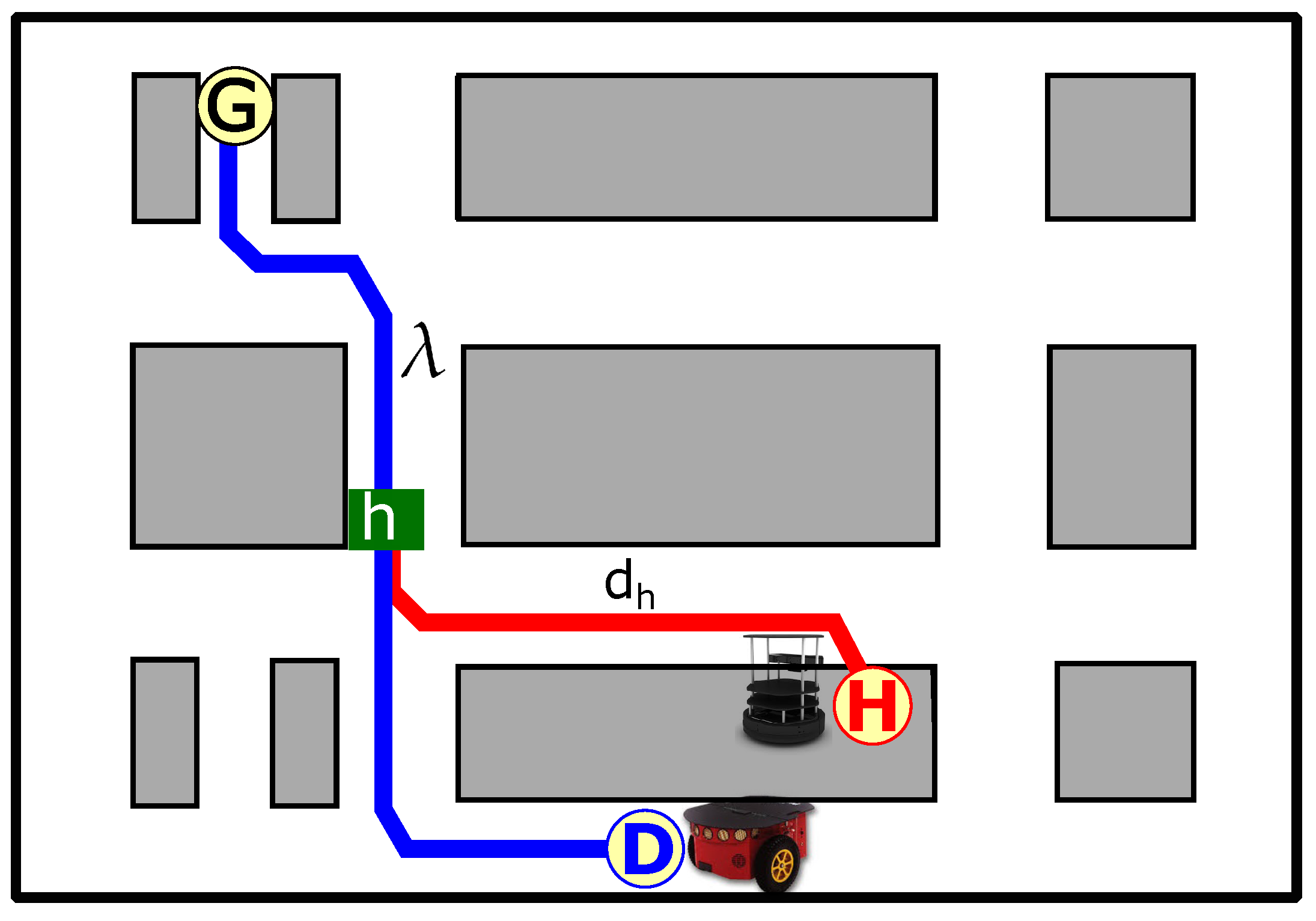
Partial hitchhiking is graphically explained in Figure 3. The hitchhiker’s start and goal locations are marked as ‘’ and ‘’, respectively. Similarly, the driver robot’s start and goal locations are marked as ‘’ and ‘’, respectively. Both of the robots have the same goal location. It can be seen that the shortest path of the driver does not pass through the hitchhiker’s location. Hence, hitchhiking is not possible in normal mode. However, the hitchhiker can self-navigate towards a location ‘’ shown in green in Figure 3, couple with the driver, and navigate together to the goal location. This is only possible in a sensor network which enables remote communication between the robots. Several areas of the map could be marked as potential hitchhiking areas that are equipped with artificial markers to facilitate coupling. In the real experiments (Section 8.2), we used corner areas as points of coupling that saved time for the robots to orient and align.
Notice that, unlike normal hitchhiking, the hitchhiker must execute its own path planning in order to calculate the point of coupling, and then navigate from the current to the coupling location on its own. Moreover, partial hitchhiking is only allowed if the length of the common path traversed (, shown in Figure 3) is larger than the threshold distance () as hitchhiking over short distances is not efficient. In Figure 3, the distance traversed by the hitchhiker is and the distance traversed symbiotically is . Partial hitchhiking is favored in scenarios with smaller and larger (given, ).
For partial hitchhiking, the point of coupling can easily be calculated in the map. Many path planning algorithms (like A-star algorithm [27]) represent the robot path in a graph structure. Let be a graph with edge distances, and be an admissible heuristic. Let be the hitchhiking point that marks the start location and be the end node of the hitchhiker robot. If is the shortest distance from to seen so far, then gives an estimate of the distance from to , and similarly from to . The queue of nodes sorted by is the A* path from to . Similarly, if is the sorted node queue of the driver robot from to , then the nearest node in is the node of coupling in the map (marked in green as ‘’ in Figure 3).
6. Multi-Driver Hitchhiking in Sensor Networks
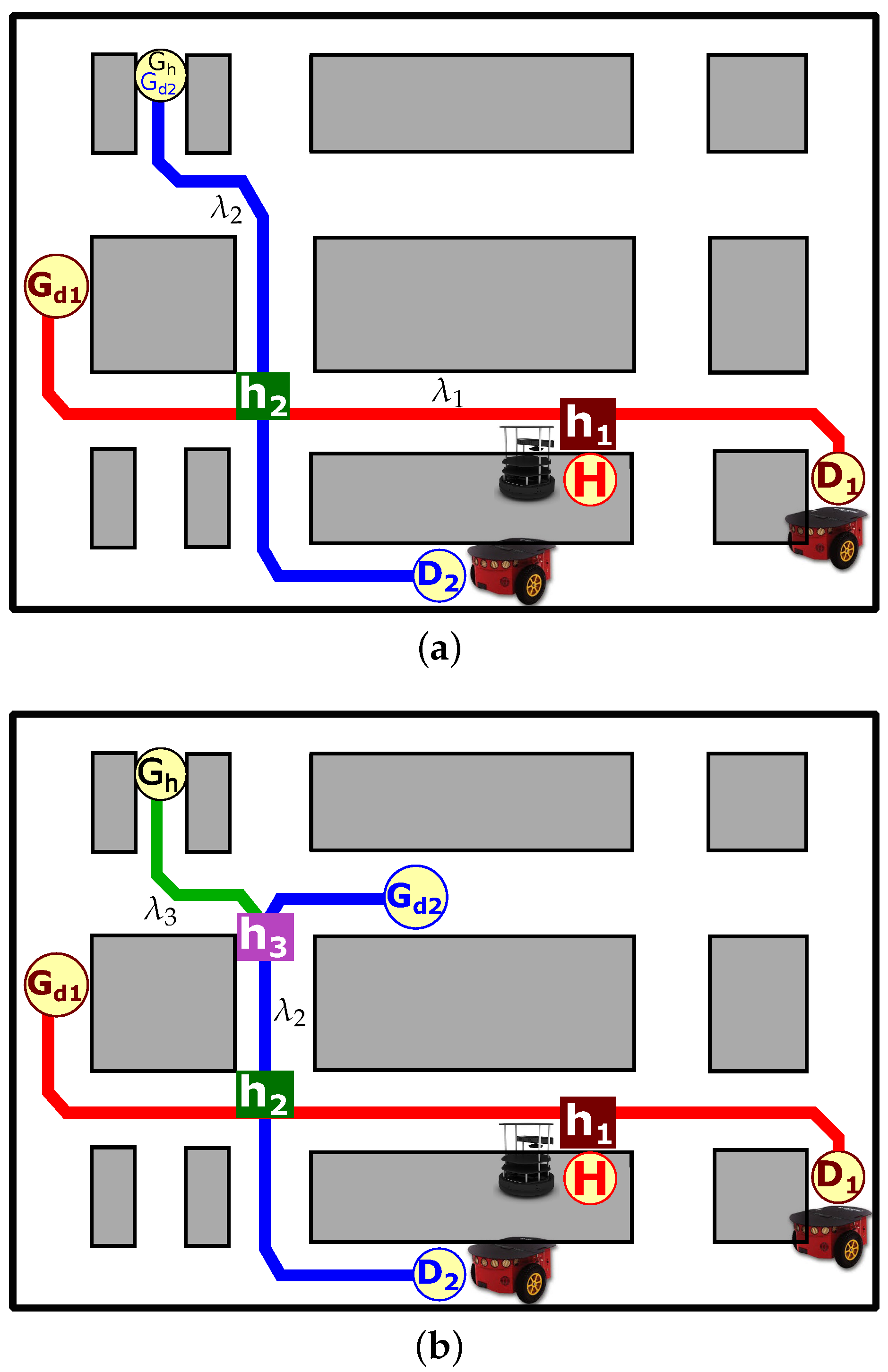
Ability to communicate with robots over long distances also enables a hitchhiker to use multiple driver robots to navigate towards its goal location. This is called multi-driver hitchhiking.
Figure 4 graphically shows the multi-driver hitchhiking scenario. In Figure 4, the hitchhiker’s start and goal locations are marked as ‘’ and ‘’, respectively. The first driver robot’s start and goal locations are marked as ‘’ and ‘’, respectively. Similarly, the second driver robot’s start and goal locations are marked as ‘’ and ‘’, respectively. In Figure 4a, and are the same locations.
In Figure 4a, there are two places of hitchhiking. The path of driver robot passes through the hitchhiker’s location and the first hitchhiking occurs at location ‘’ marked in brown. Driver and hitchhiker decouple at location marked in green. The location falls in the path of the second driver shown in blue. The hitchhiker then waits for the robot and navigates with it to the goal location .
Figure 4a showed a scenario with a common goal between the driver and the hitchhiker. On the contrary, Figure 4b shows a scenario with different goals of the driver and the hitchhiker. In the latter case, the first hitchhiking starts at location ‘’ marked in brown with driver , and the second hitchhiking at location ‘’ marked in green with driver . Since driver ’s goal is different () from the hitchhiker’s goal (), the hitchhiker decouples at location from where the hitchhiker navigates towards the goal using its own modules.
Just like partial hitchhiking, the hitchhiker also needs to plan a path using its own path-planning module in a multi-driver hitchhiking scenario. Let , , and be the node paths of the hitchhiker, driver 1, and driver 2, respectively. In the scenario of Figure 4b, the two points and are given by,
The path traversed by the hitchhiker during the first and second hitchhiking are and , respectively. Notice that in both cases in Figure 4a,b, hitchhiking is allowed only if and . In a sensor network, a time synchronization is required between the robots. Particularly, the second driver could arrive at the second hitchhiking location before the robots and , and must be ready to wait for them, and vice-versa.
7. Multi-Robot Teleoperation through Hitchhiking in Sensor Networks
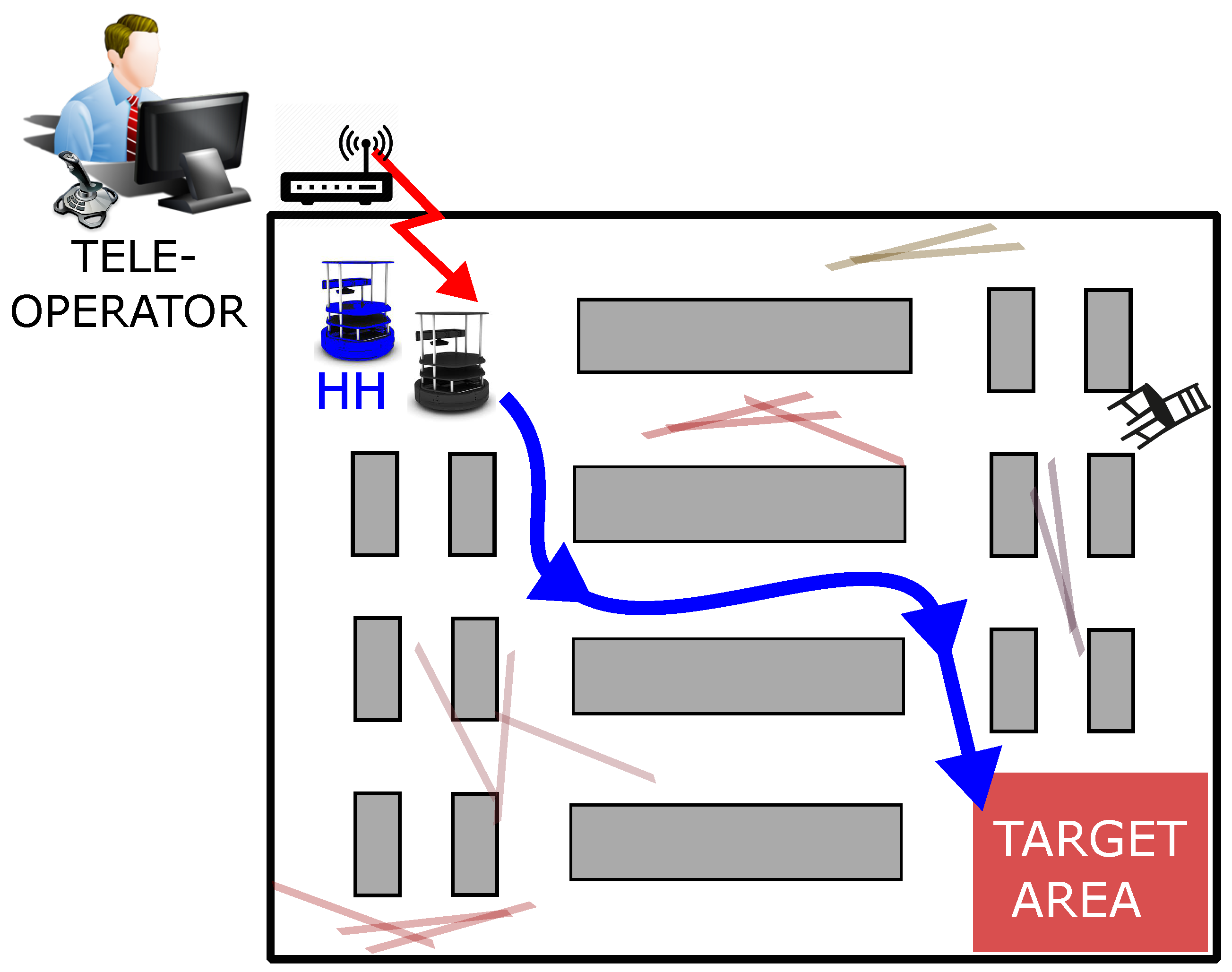
Hitchhiking can also assist in simultaneous teleoperation of multiple robots by a single teleoperator. Although robots are getting more and more autonomous in their tasks, some tasks like search and rescue operations at disaster sites require a human to be in control and navigate the robots. In these tasks, multiple robots are often teleoperated and navigated to specific areas of the map. The robots are generally equipped with cameras that capture a live video that is relayed to the teleoperator. The teleoperator then controls the robot motion through input devices like joysticks or wearable sensors.
Although the teleoperation of a single robot is easy, it is difficult to simultaneously teleoperate multiple robots by a single operator. Hitchhiking can be useful to assist with simultaneous teleoperation of multiple robots. Figure 5 shows a scenario of a disaster site in which two robots are to be navigated to the marked target area. This is a common scenario in which multiple robots carry first-aid or necessary items to the target area. In such scenarios, the teleoperator can control only one robot, while the other robot could hitchhike and follow the other robot using the QR-code and camera setup. This is graphically shown in Figure 5 in which the teleoperator only controls the black robot, while the blue robot hitchhikes and follows the driver robot towards the common target area.
Teleoperating multiple robots using hitchhiking has several advantages compared to normal hitchhiking:
- There is an ease of simultaneously teleoperating multiple robots towards a common goal by a single teleoperator. It eliminates the need of using multiple operators, or separately controlling the robots one-by-one.
- It saves time as both the robots are simultaneously controlled and navigated in the area.
- It eliminates redundant control operations. In the absence of hitchhiking based teleoperation, the operator would have to repeat the same set of commands for each robot. However, in hitchhiking based teleoperation, the redundant commands to the robots are eliminated, and only one robot is effectively controlled.
- It saves network bandwidth as only one robot needs to be sent the commands from the teleoperator.
8. Experimental Results
We performed experiments in both simulation and real environment to test the benefits of hitchhiking in sensor networks.
8.1. Experiments in Simulation Environments
The simulation was programmed in Matlab software (R2011b, MathWorks, Natick, MA, USA) and is shown in Figure 6. The path planning algorithm used was D-Star algorithm [28,29]. The simulation environment is comprised of a grid map with obstacles shown in gray. In the grid map, the cost of navigating one micro-grid in forward, back, left, and right direction was set to one unit. For diagonal movement, the navigation cost was set to units. The scale of the map was set as 1 m = 4 grid pixels.
The simulation was carried with three driver robots and one hitchhiker robot. In Figure 6, , , and mark the starting positions of the three potential driver robots, the hitchhiker robot is marked as , and the goal location is marked as . The hitchhiking spot is marked with a yellow circle and the common path is also shown in Figure 6.
8.1.1. Worst Case Scenario with No Potential Drivers
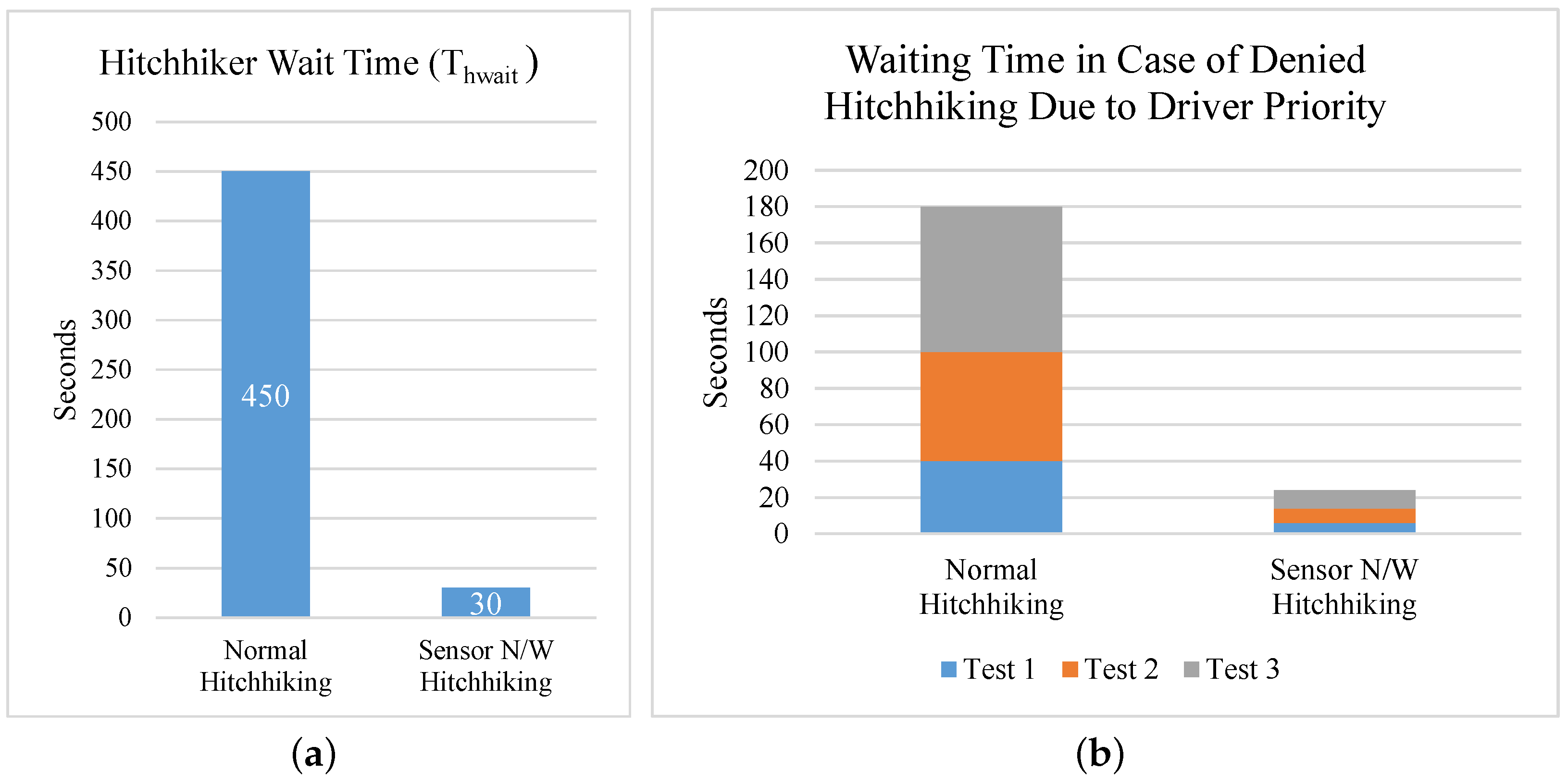
The worst case scenario in hitchhiking is when there are no potential drivers and the hitchhiker has to wait. In the simulation, we set the threshold waiting time () to 150 s. In the absence of a sensor network, the hitchhiker had to wait a total of 450 s in three test runs. This is shown in Figure 7a. However, in a sensor network, the robot could quickly confirm the non-availability of potential drivers and navigate towards its goal using its own modules. Considering the delay in communication, and parsing the messages set to 10 s, the total waiting time in sensor environment hitchhiking was only 30 s, and the hitchhiker navigated to the goal on its own.
8.1.2. Denied Hitchhiking Due to Driver Priority
Potential drivers navigating to the same location as the hitchhiker and with higher profiles may still deny hitchhiking if they have a high priority (time-critical) task at hand. We tested this case in a simulation environment with three driver robots at a speed of 0.5 m/s. The three driver robots were 80, 120, and 160 grid-pixels from the hitchhiker (equivalent to 20 m, 30 m, and 40 m, respectively). As shown in Figure 7b, in the absence of a sensor network, the hitchhiker had to wait for a total time of 180 s. However, in the presence of a sensor network, the hitchhiking was denied from remote locations with only a little time (24 s) spent on communication.
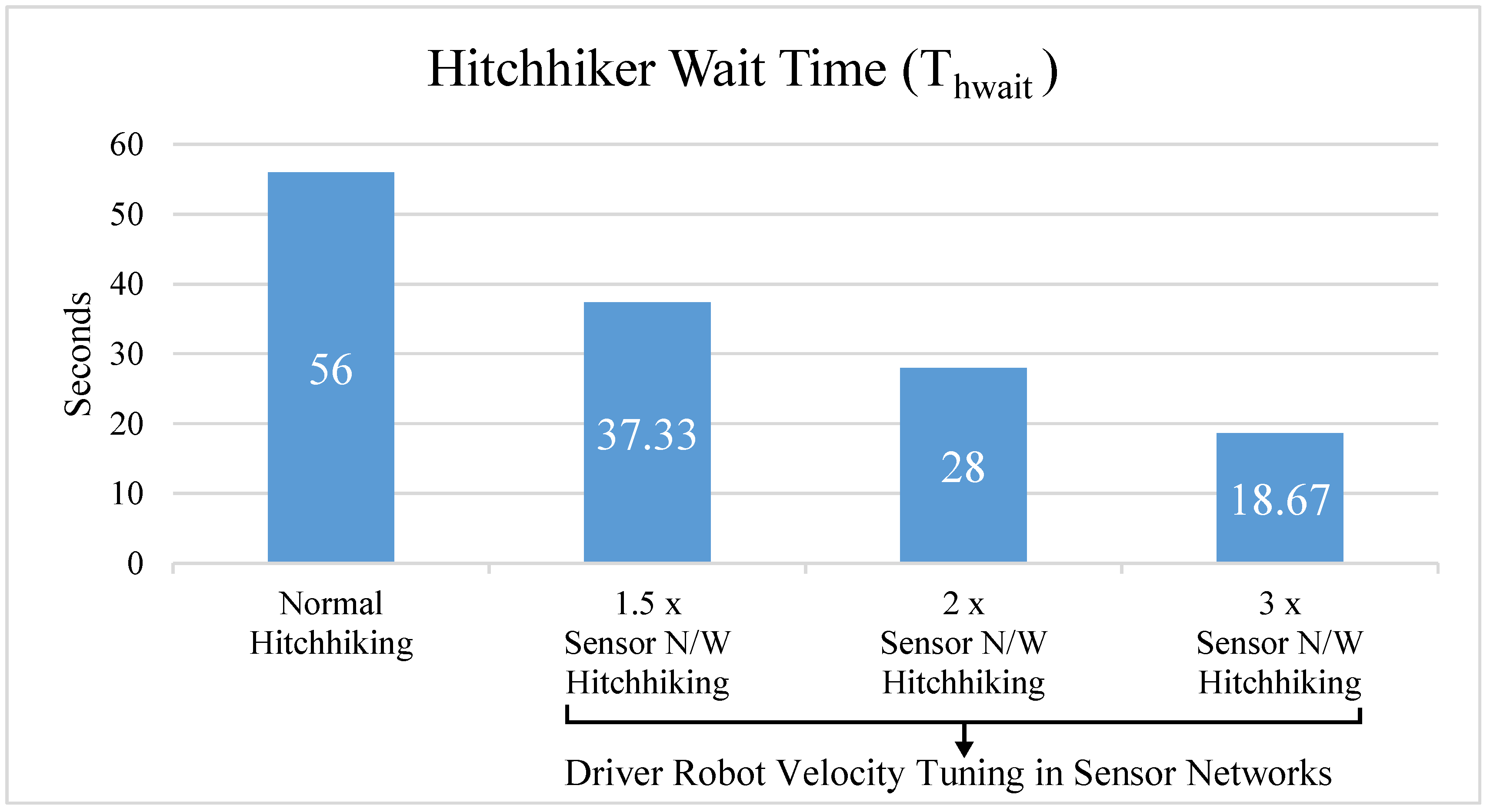
8.1.3. Velocity Tuning of Potential Drivers
With the threshold waiting time () set to 150 s, the velocity of driver was set to 1 m/s (4 grid-pixels/s). As shown in Figure 6, the distance between and is approximately 225 grid pixels (≈56 m). Thus, in simulation without a sensor network, at a normal speed of 1 m/s, the robot took 56 s to reach the hitchhiker. However, in the sensor network, the request was processed from a remote location and the driver robot increased its speed to reach the hitchhiking spot early. Figure 8 shows the waiting time of a hitchhiker with a driver robot increasing its speed by , , and . The hitchhiker’s waiting time is inversely proportional to an increase in driver’s speed.
8.1.4. Best Profile Match
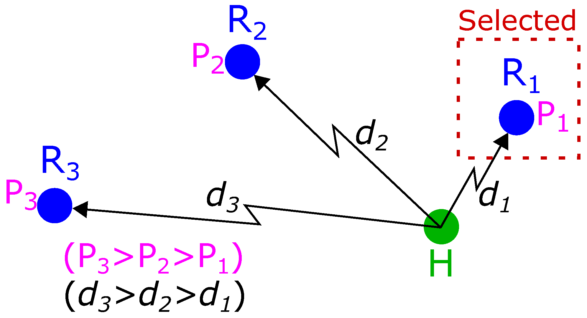
Three driver robots () were simulated in the environment shown in Figure 6 with varying distances , and from the hitchhiker (), respectively, in all possible combinations. The driver robots were also assigned varying profile scores , and , respectively. In the absence of sensor networks, only the robot with the shortest distance was selected, irrespective of the profile of the robot. The results of different distance configurations (e.g., ) are given in Table 1. It can be seen that in case of hitchhiking without a sensor network, only the nearest potential driver is selected, which may be wrong. This is explained in Figure 9, which shows a configuration with . Although robot has the highest profile score (), robot is still selected as a potential driver for hitchhiking as it is closest to the hitchhiker and approaches the hitchhiker prior to the other robots with better profiles. However, in a sensor network, the robot with the highest profile score is always selected as shown in Table 1.
8.2. Experiment in a Real Environment
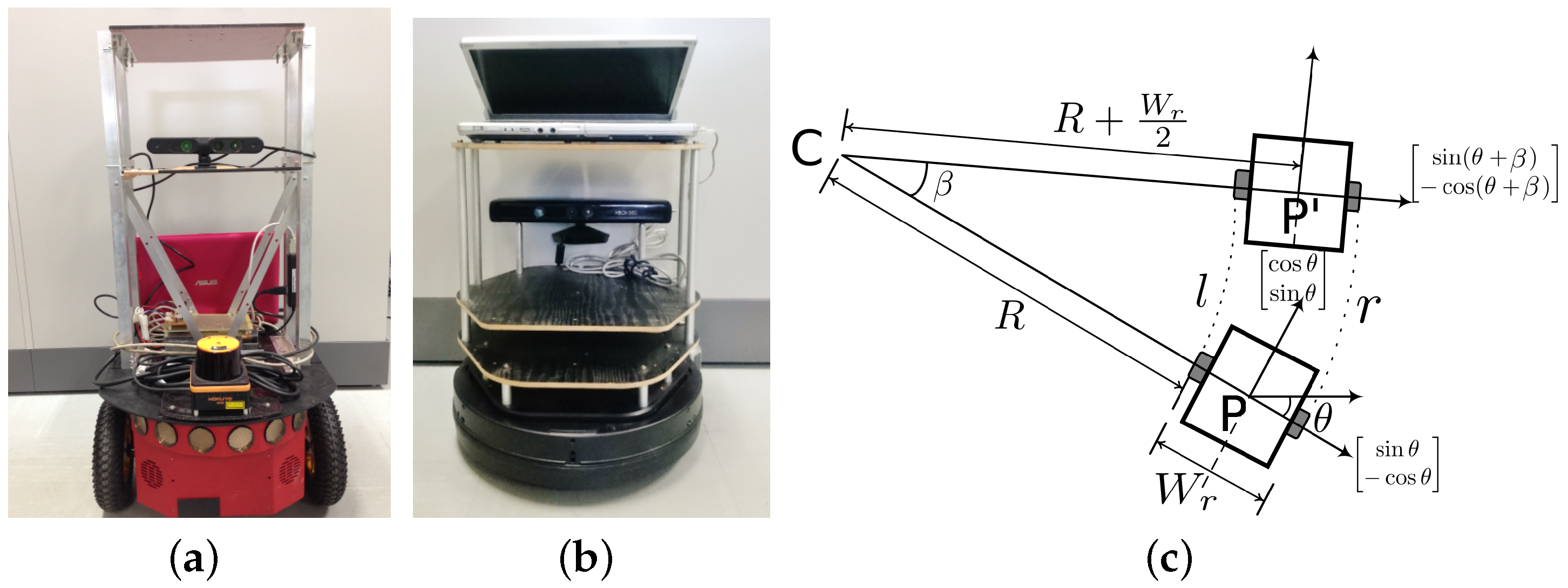
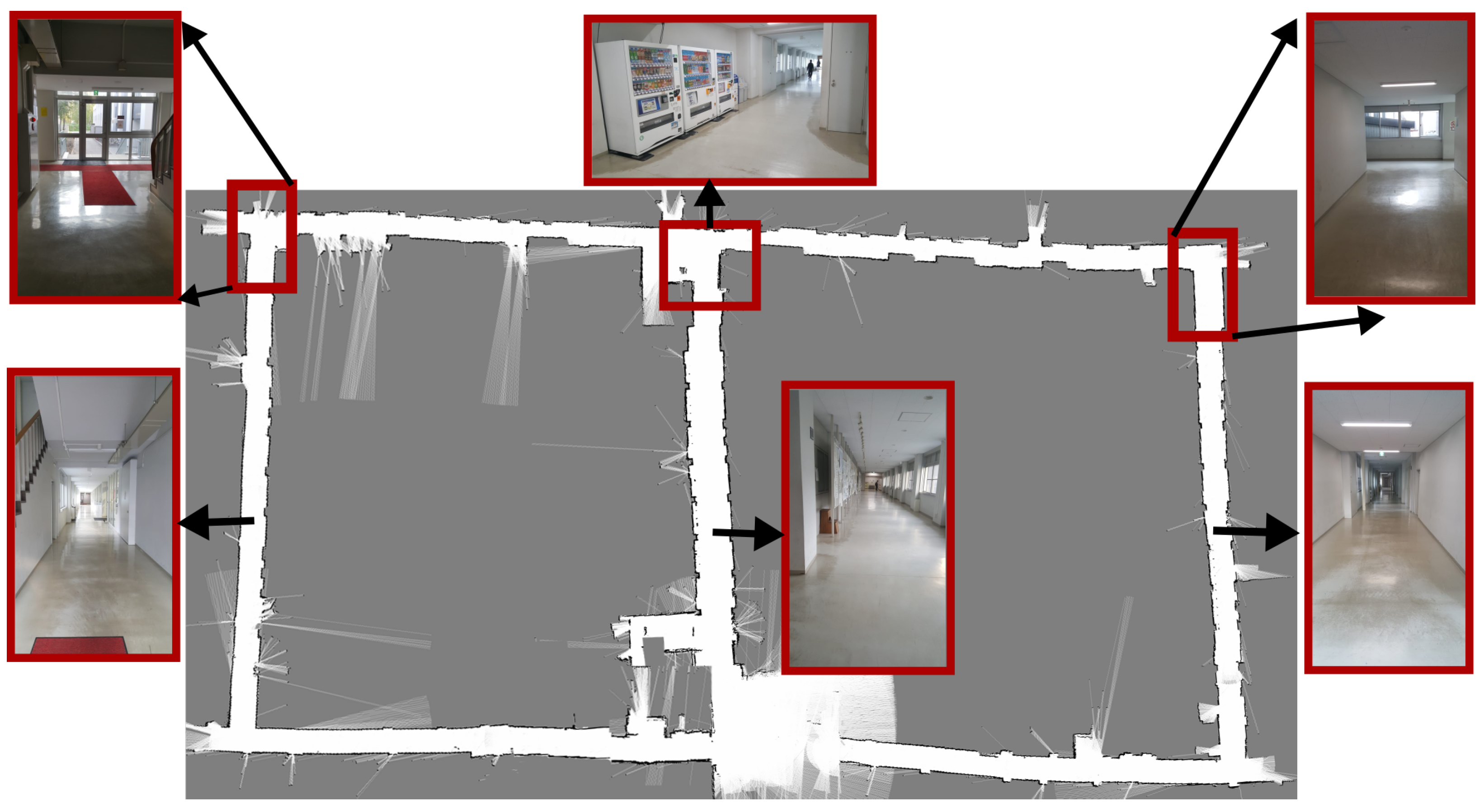
Two robots Pioneer-P3DX (Figure 10a) [30] and Kobuki Turtlebot (Figure 10b) [31] were used, which were equipped with distance sensors (Microsoft Kinect [32] and UHG-08LX laser range sensor [33]) and cameras. The experiment environment is shown in Figure 11. The distance sensor is accurate within mm within 1 m, and within 3% of the detected distance between 1 and 8 m. The angular resolution is approximately 0.36 degrees, and other specifications can be found in [33]. The driver robot was Pioneer P3DX, and Turtlebot was the hitchhiker. The robots were programmed in ROS [34]. The sensor network was set to enable remote communication between robots. A modified open source library [35,36,37] was used for visual servoing. Both are differential drive robots, and their motion model is well known [17]. A-star algorithm [27] was used for path planning. Five experiments in real environments were performed for: (1) Normal hitchhiking, (2) Partial hitchhiking, (3) Multi-driver hitchhiking, (4) Hitchhiking based teleoperation, and (5) Denied hitchhiking in sensor networks, which are explained in the next subsections.
8.3. Integrating Hitchhiking with an EKF Based SLAM Algorithm
We first describe the motion model of the robot. The distance between the left and the right wheel is , and the robot state at position P is given as []. From Figure 10c, turning angle is calculated as
and the radius of turn R as
The new heading is
from which the coordinates of the new position are calculated as
If , i.e., if the robot motion is straight, the state parameters are given as , and
EKF is a mathematical tool to model the uncertainties of the sensors attached to the robot. It can be used with different sensors and a complete description is given in [38].
The state of the robot () at time t is indicated by a vector comprised of its pose and orientation () as . EKF assumes a Gaussian distribution in which the belief at time t is given by the mean and the covariance . A command moves the robot comprising of the translation velocity () and rotational velocity () as :
EKF uses Jacobians of motion and control functions to deal with the nonlinearity of the system. The Jacobian of motion function with respect to state is given by
and the Jacobian of motion with respect to control is given by
With robot specific error-parameters , the covariance of noise in control space is given by
Here, are robot specific parameters. They are determined empirically and vary from robot to robot [38]. The prediction updates in state () and covariance () are given by
and
respectively. The mapping from motion noise in control space to motion noise in state space is provided by the term in Equation (12).
To model the correction step, we assume that the sensors provide the range (), bearing (), andsignature (, e.g., color) of the landmark relative to the robot’s current pose (). The covariance () of the sensor noise is given by the matrix
Let be the coordinates of the ith landmark obtained by measurement from the current pose , and q represent the squared distance as
Then, we have
The Jacobian of measurement with respect to state is given by
This gives the measurement covariance matrix as
Maximum likelihood estimate is applied for all the k landmarks (Equations (14)–(17)) in the map to calculate the most likey correspondence as
The calculation of Kalman gain () and EKF updates for state () and covariance () only corresponds to this most likely estimate:
Thus, at each time step (t), a Kalman gain () is calculated from which the state () and covariance () are updated by the robot. In traditional navigation schemes, each robot of the multi-robot system must execute localization using the abovementioned computationally expensive steps.
In hitchhiking, the driver robot executes localization using the steps described above. The hitchhiker follows the driver through visual servoing and shuts down the SLAM module. However, during decoupling, the driver must transfer its pose so that the hitchhiker knows where it is currently in the map. This is to ensure that the hitchhiker can localize at the decoupled location and navigate to other places on its own. Failing to do this would result in the hitchhiker being in a completely unknown place. This scenario is often known as the ‘kidnapped robot problem’, and this problem is avoided by transferring the driver’s pose to the hitchhiker.
During decoupling, the driver transfers its pose () to the hitchhiker robot and the uncertainty associated with it (). The final orientation of the hitchhiker () is same as that of the driver robot as the hitchhiker follows the driver using the QR-code and camera setup which tries to be inline, i.e.,
If d is the distance between the hitchhiker and the driver during decoupling, then the pose of hitchhiker is given as
Moreover, the hitchhiker assumes the same uncertainty in its pose as the driver robot, i.e.,
The hitchhiker robot uses this pose () to localize itself in the map. It can use the uncertainty () information to consider the distribution of particles (e.g., in case of particle filter [38,39,40,41]) by taking the eigenvalue-eigenvector decomposition of . Eigenvalues () and eigenvectors () of the matrix gives the magnitude and direction of variance, respectively, for considerable distribution of particle poses.
8.3.1. Experiment 1: Full Hitchhiking in a Sensor Network (with Velocity Tuning)
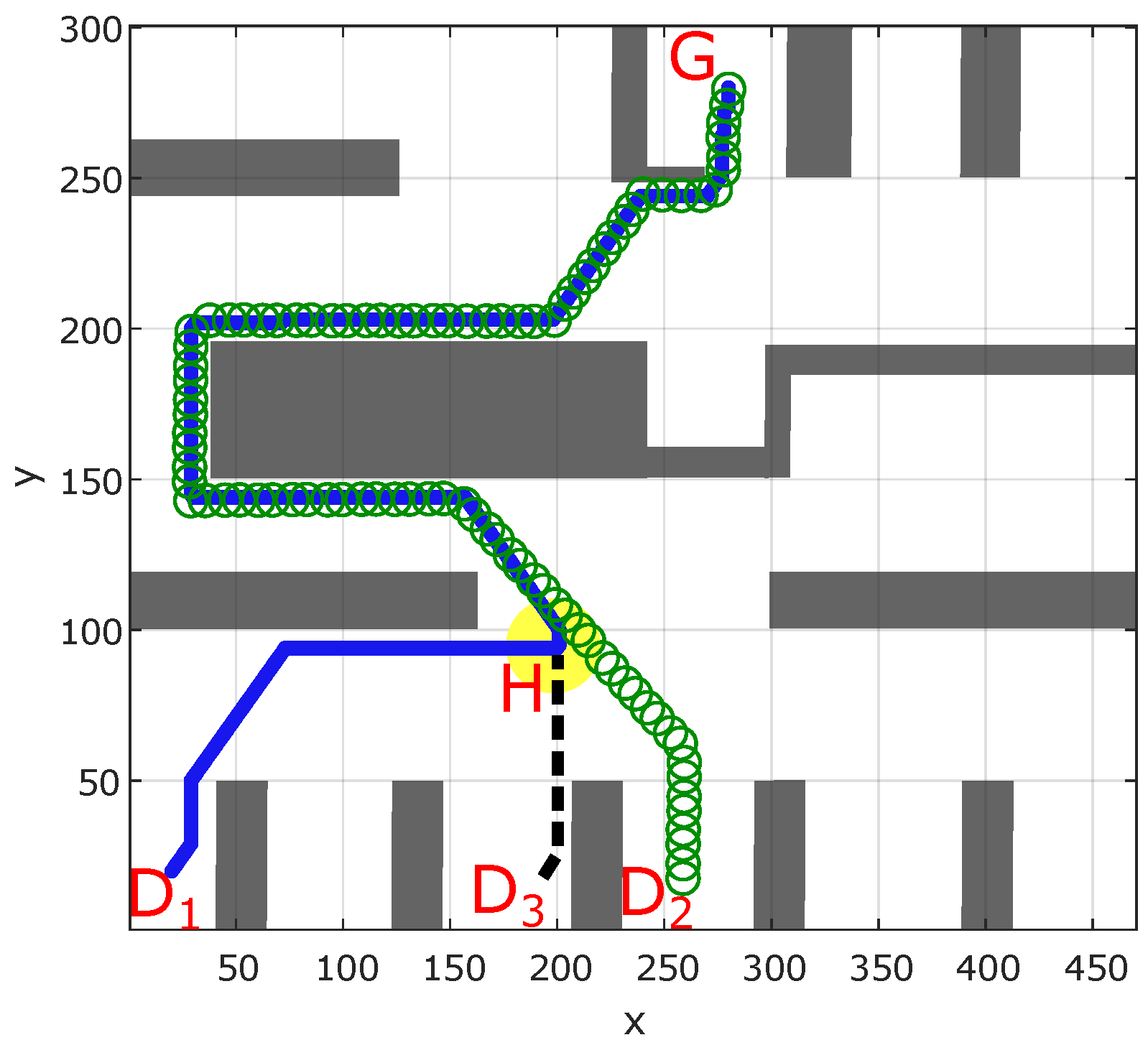
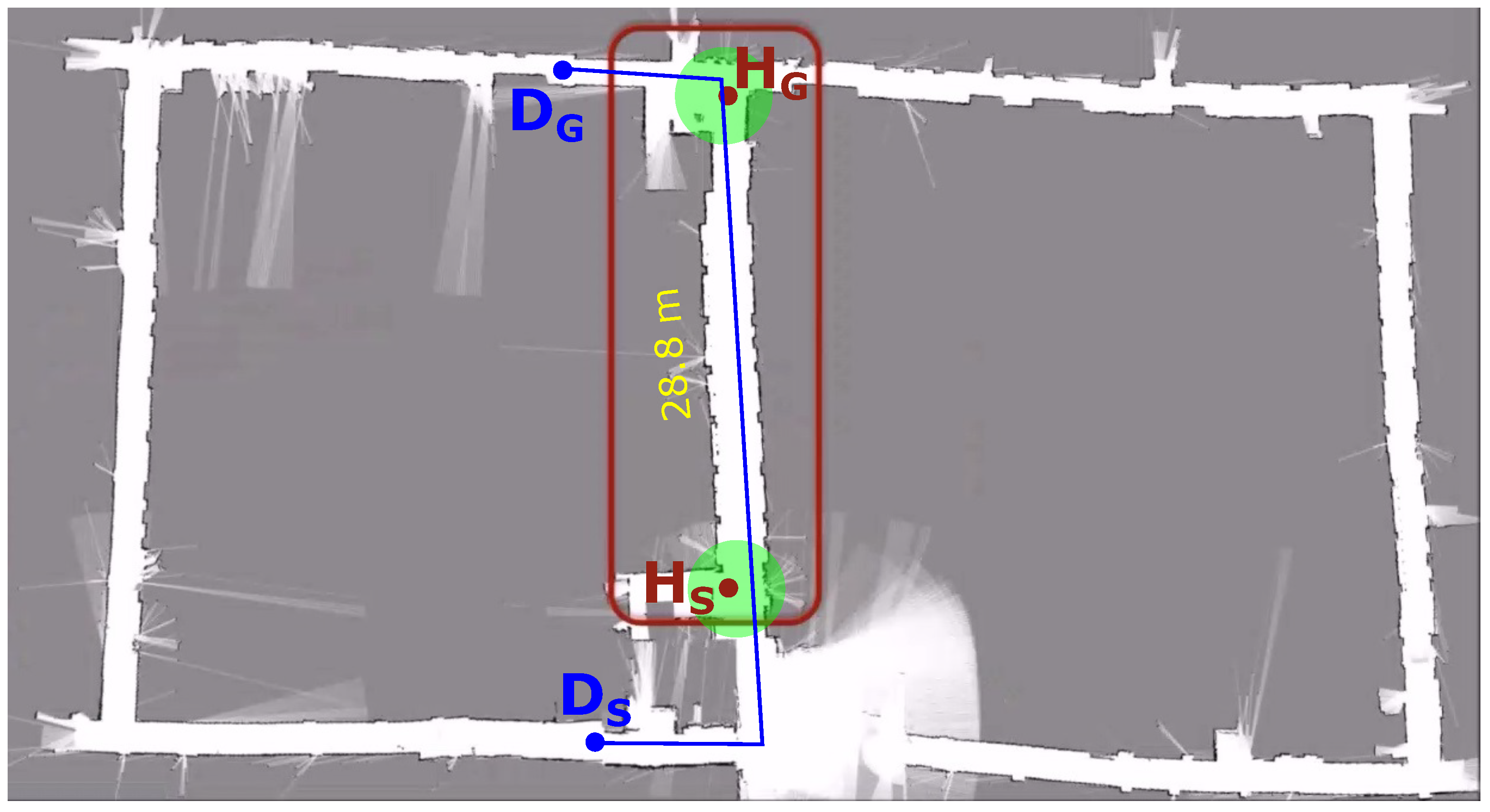
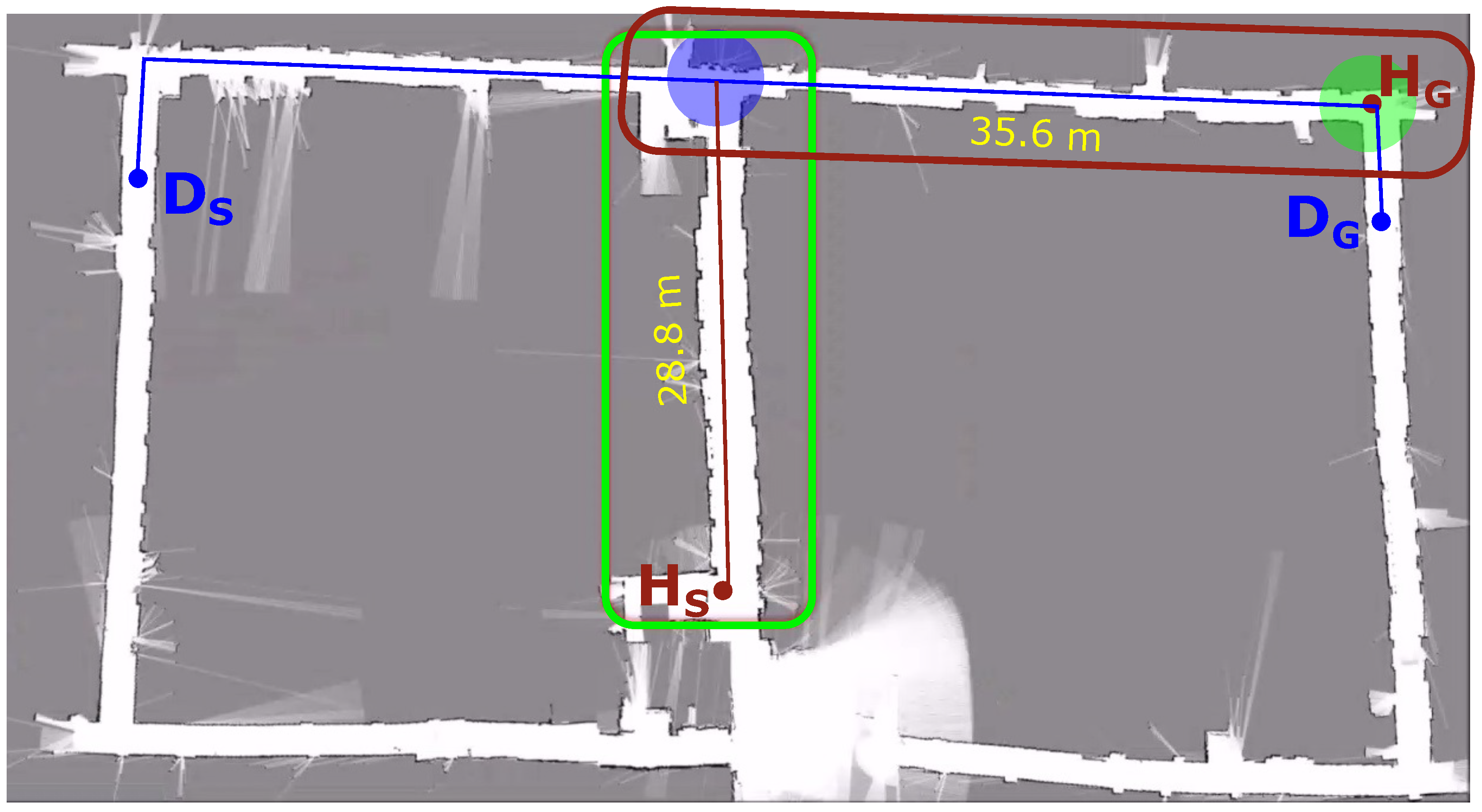
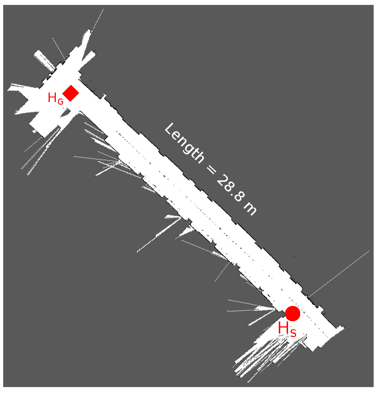
We tested the proposed algorithms on the ground floor of the engineering building of Hokkaido University, which is comprised of many interconnecting passages (Figure 11). The grid map of the environment is shown in Figure 12. In Figure 12, the start and goal locations of the hitchhiker are marked in red as and , respectively. The total hitchhiking distance was equal to the length of the corridor (≈28.8 m). The driver’s start and goal locations are marked in blue as and , respectively. The path planned by the driver robot is indicated in blue and passes through the hitchhiker’s location. Moreover, the goal location of the hitchhiker also falls on the path of the driver. Hence, this is the perfect scenario of full hitchhiking. The coupling and decoupling areas are marked as green circles in Figure 12.
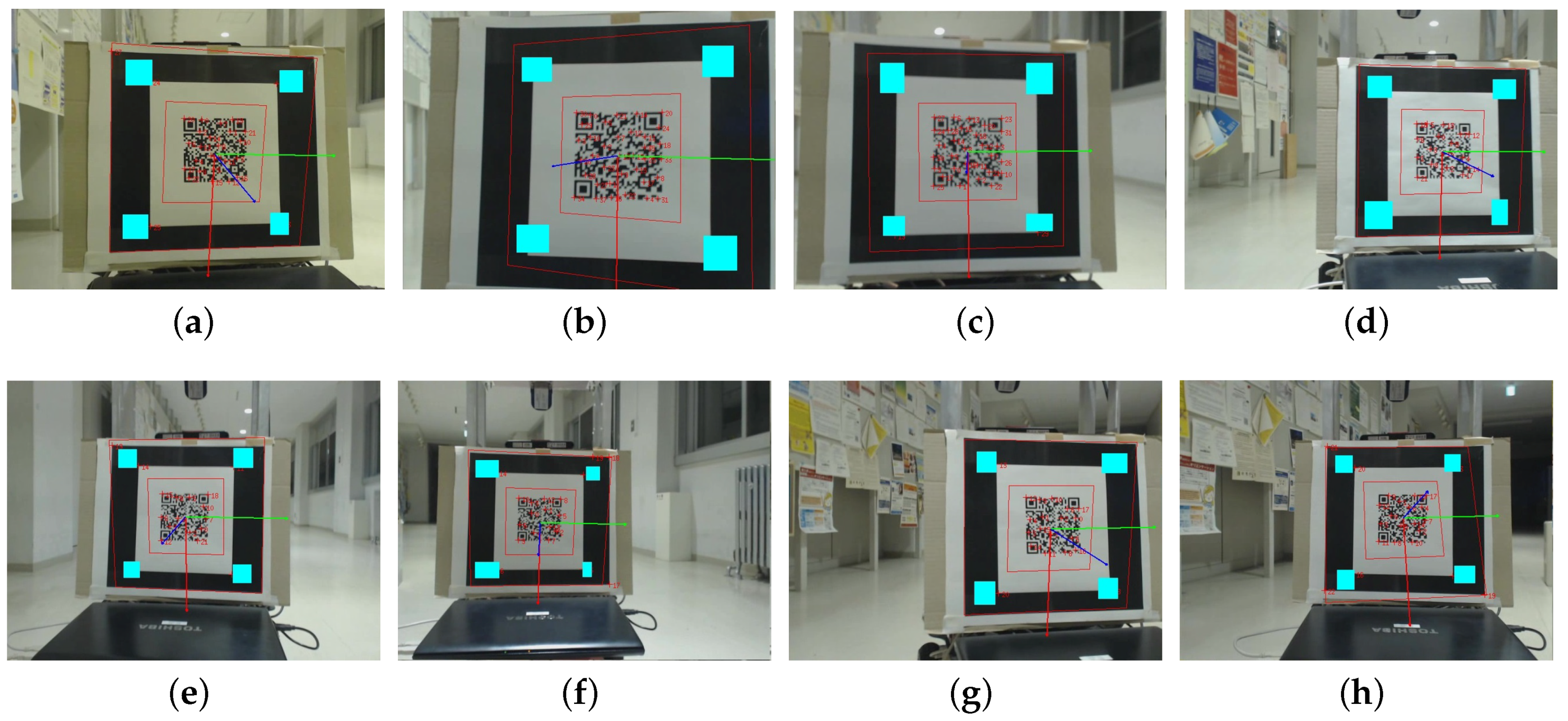
Unlike the hitchhiking proposed in [2], the hitchhiker was able to lock the driver robot for hitchhiking remotely. This also enabled testing the velocity tuning of driver robot, and the driver robot increased its speed from 0.5 m/s to 1.0 m/s (within the safe velocity threshold of a Pioneer P3DX robot) from to . Doubling the driver’s speed reduced the hitchhiker’s waiting time by 50% from ≈10 s to 20 s. Figure 13 shows the random frames of visual servoing from to at different locations.
8.3.2. Experiment 2: Partial Hitchhiking
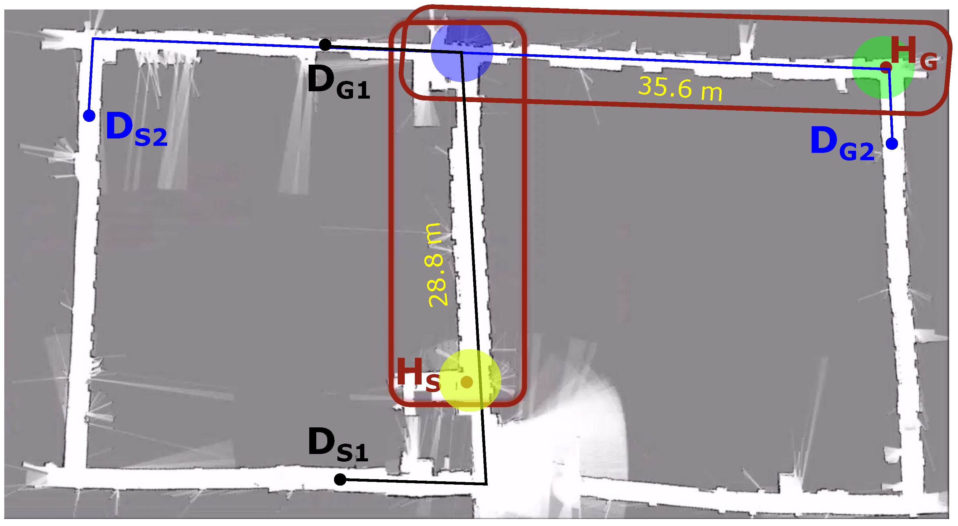
We tested partial hitchhiking in the same environment. The partial hitchhiking scenario is shown in Figure 14. The hitchhiker’s start and goal locations are marked as and , respectively. The driver’s start and goal locations are marked as and , respectively. The driver robot’s path is indicated in blue. Notice that the driver’s path does not pass through the hitchhiker’s location. Hence, normal hitchhiking [2] was not feasible. However, the paths of the two robots intersect, and the common path was large enough for partial hitchhiking. The hitchhiker thus navigated towards the point of intersection of the paths of the hitchhiker and the driver, which is indicated with a blue circle in Figure 14. The hitchhiker and driver coupled at the location are shown with a blue circle in Figure 14, and are then decoupled at the hitchhiker’s goal location marked with a green circle.
In this experiment, the hitchhiker traversed a distance of approximately 28.8 m marked with a green rectangle in Figure 14. The distance navigated through hitchhiking was approximately 35.6 m and is marked with a brown rectangle. Since the hitchhiked distance was larger than the threshold distance ( m), partial hitchhiking was feasible. Both the hitchhiker and the driver robots started navigation at the same time from their respective start locations.
8.3.3. Experiment 3: Multi-Driver Hitchhiking
Figure 15 shows the environment setup for multi-driver hitchhiking. The hitchhiker’s start and goal locations are marked as and , respectively. The first driver’s start and goal locations are marked in black as and , respectively. The first driver robot’s path is indicated in black. Similarly, the second driver’s start and goal locations are marked in blue as and , respectively. The second driver robot’s path is indicated in blue.
In this setup, the first driver’s path passes through the hitchhikers location. Hence, hitchhiking first took place at the location marked in yellow circle in Figure 15. The decoupling location is the point of intersection of the hitchhiker’s path and the second driver’s path is shown in blue, which is also the point of second hitchhiking with the second driver.
In this experiment, the hitchhiker traversed a distance of approximately 28.8 m through the first hitchhiking. The distance navigated through the second hitchhiking was approximately 35.6 m and is marked with a brown rectangle. In both cases, the hitchhiked distance was larger than the threshold distance ( m). Multiple hitchhiking was feasible since the status and path information of both the drivers were acquired by the hitchhiker in the sensor network. In this experiment, both the driver’s and were programmed to start simultaneously. Hence, driver reached the location marked with the blue circle before the hitchhiker. For time synchronization, we simply programmed the second robot to wait until the hitchhiker had arrived. Driver had to wait for ≈21 s.
8.3.4. Experiment 4: Hitchhiking Based Simultaneous Multi-Robot Teleoperation
The same setup shown in Figure 12 was used to test the simultaneous teleoperation of two robots using a single teleoperator. The section of the teleoperated portion of the map is shown in Figure 16. As with the previous experiments, Pioneer P3DX was set as the driver robot and was directly teleoperated using a keyboard. Turtlebot was the hitchhiker and followed the driver. The hitchhiking location was and the goal location was set to shown in Figure 12. The teleoperator was successfully able to simultaneously navigate both of the robots to the desired location by controlling only one of the robots.
8.3.5. Experiment 5: Denied Hitchhiking in a Sensor Network
We repeated the experiment described in our previous work (Section 7.3 of [2]) to test cases in which hitchhiking should be denied. Similar to [2], we set the hitchhiker with a profile score () of 90, and driver with a profile score () of 58. Clearly, hitchhiking must be denied in this case as . The waiting time () was set to 25 s. In traditional hitchhiking [2], the robot waited for seconds until the driver was in proximity for communication and later the hitchhiking was denied. However, in a sensor network case, the hitchhiker knew about the low profile score of the driver from the remote location and continued to navigate towards the goal using its own module without hitchhiking. Namely, although the hitchhiking was denied, a sensor network enabled the hitchhiker to know quickly that there are no potential drivers and it saves on waiting time.
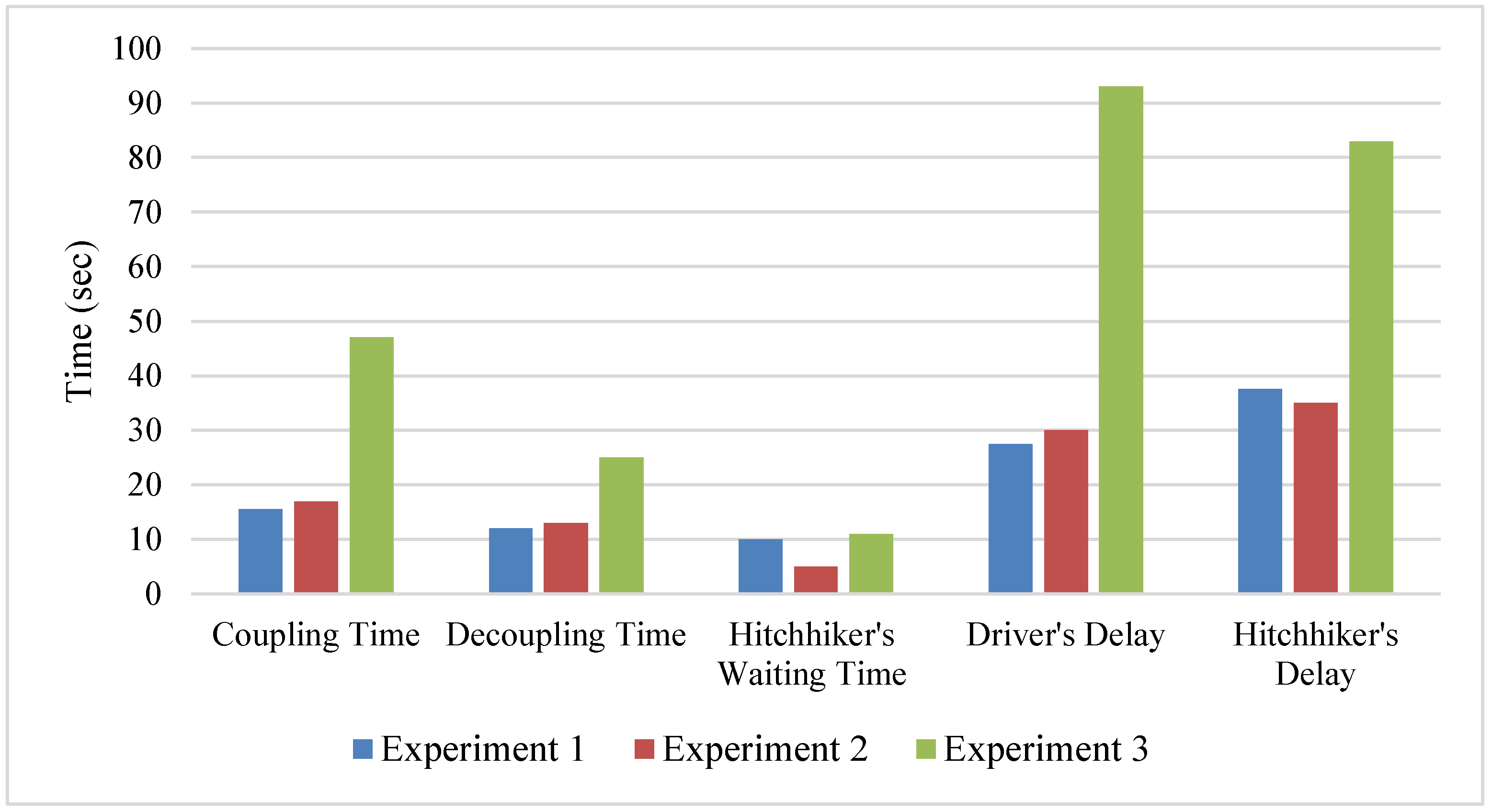
Figure 17 summarizes the total time required for coupling, decoupling, hitchhiker’s waiting time, driver’s delay, and hitchhiker’s delay in Experiments 1 (full hitchhiking), 2 (partial hitchhiking), and 3 (multi-driver hitchhiking). Table 2 provides the breakdown of the various times. On average, it took about 15 s for coupling and decoupling. However, in the multi-driver experiment, the second driver took more time to properly align as the hitchhiker had to first decouple from the first driver and then couple with the second driver. Hence, the alignment took extra time. In Table 2, in the multi-driver experiment, there is no waiting time () for the hitchhiker for the second hitchhiking as the second driver had already positioned itself and the hitchhiker did not wait for the second driver. For the same case, the second driver’s delay was 65 s as it included its waiting time of ≈21 s at the location marked with the blue circle in Figure 15 of Experiment 3.
Table 3 shows the different modules run by the two robots while navigating in the normal hitchhiking case. It is clear that the traditional navigation requires all the modules of both the robots to be active. On the other hand, in hitchhiking, most of the modules of the hitchhiker are off. One overhead is visual servoing, which is not computationally expensive compared to SLAM (especially 3D SLAM). Similarly, Table 4 shows the modules run by the two robots while navigating in a traditional and partial hitchhiking case. The traditional navigation requires both robots to execute all the modules, whereas in partial hitchhiking, the hitchhiking robot executes these modules only for a portion of the path. In Table 3 and Table 4, the modules which are either off or executed partially have been indicated in red color. Although costs are incurred in coupling and waiting, in both the cases, hitchhiking is only allowed if the common path of the driver and hitchhiker robots are larger than the threshold distance () and denied otherwise (Algorithm 2, lines 2–3) to ensure efficiency.
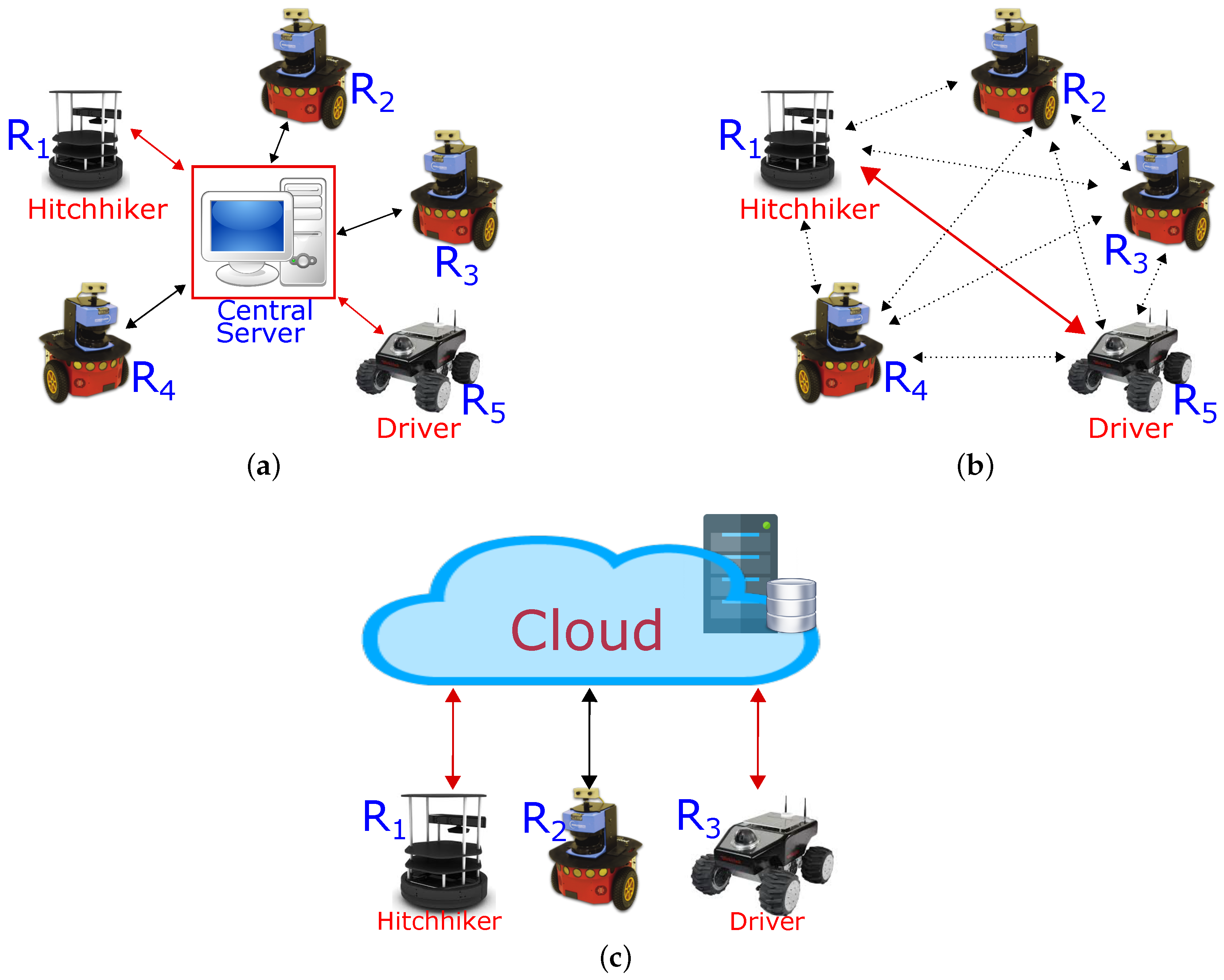
9. A Note on System Architecture for Multi-Robot Hitchhiking
Inter-robot communication is an indispensable part of a hitchhiking system. Although inter-robot networking is not the main research or contribution of this work, for the sake of completeness, a short note on some prominent system architectures with their advantages and disadvantages are provided in this section. Multi-robot hitchhiking could be implemented through various system architectures. Figure 18 shows three such prominent architectures: (a) Centralized architecture (Figure 18a), (b) Distributed architecture (Figure 18b), and (c) Cloud architecture (Figure 18c). The discussion is restricted to the implementation of hitchhiking robots only.
Figure 18a shows a central architecture in which various robots () communicate through a central server. Thus, a hitchhiker robot would communicate with a potential driver () through the central server. For a multi-robot system, this architecture is easy to implement. A powerful centralized server has an advantage that robots can delegate some of their heavy computational tasks to the server (e.g., path planning). However, a failure of the central server would entirely disable the entire system. Moreover, in the context of a multi-robot hitchhiking system, it is not always feasible to dedicate a separate system for the central server.
Figure 18b shows a distributed architecture. All the robots () have the capability of directly communicating with each other. In other words, each node must be a server as well as a client, and hence it seems to be a complex system to setup. However, notice that ROS (Robot Operating System) has a strong in-built support for establishing such a network. The details of establishing such network have been detailed in [42,43]. For most of the indoor service robots, a local ROS network is sufficient. For outdoor scenarios, approaches like creating a bridge, or port forwarding as discussed in [43] could be employed. A distributed architecture using ROS was used in all the experiments in the proposed work. Fault tolerance and cost-effectiveness were the primary reasons for selecting this architecture in our implementation.
Figure 18c shows a cloud based architecture. Although it has not been incorporated in the proposed system, recently there have been many promising projects utilizing this architecture like Rapyuta [44] the cloud engine for RoboEarth [45,46,47,48,49], RobotWebTools [50], and others. The challenges of cloud robotic systems have been discussed in [51]. In the context of hitchhiking robot system, the primary disadvantage of a cloud based architecture is network latency. For indoor robots, a peer-to-peer network can easily be set up and setting a cloud system is an overkill. For example, a direct communication between the hitchhiker and the driver robots in proximity for coupling and decoupling is straightforward, whereas a cloud based system would only induce latency. This will have adverse effects on the quality-of-service.
10. Discussion and Conclusions
One of the most profound advantages that robots can have in a sensor network is the ability to communicate their status (e.g., current location, goal locations, planned paths, etc.) remotely with other robots. Our earlier worked showed the feasibility of hitchhiking, and advantages of cooperative navigation of two robots towards the same (or close) goal locations. However, it had many constraints due to a communication bottleneck. We showed that hitchhiking in a sensor network removes those constraints and improves the ability of multiple robots to symbiotically navigate together. A sensor network enables remote communication and enables partial and multi-driver hitchhiking. There is a reduced waiting time of the hitchhiker robot, and the potential driver robot with the best profile is selected. Moreover, the driver robot is able to tune its velocity within the safety limits to further reduce the hitchhiker’s waiting time. Even in case of denied hitchhiking due to any of the reasons, a sensor network enables the hitchhiker to quickly know the status and avoid unnecessary waiting. We showed that it is not necessary for the robots to have exactly the same start and goal locations. In fact, partial hitchhiking allows a hitchhiker to navigate a portion of the path on its own, and some of the path symbiotically. In this regard, a sensor network enables the robots to be able to couple and decouple at different positions in the map. Moreover, this also enables a hitchhiker robot to utilize different driver robots to navigate towards its goal.
It should be noted that additional costs are incurred in hitchhiking in coupling (aligning) the driver and hitchhiker robots, and waiting. However, efficiency is ensured by only allowing hitchhiking over large distances () and denying hitchhiking for high-priority tasks. Our work is focused on the feasibility of hitchhiking based multi-robot navigation in a sensor network and not on energy saving techniques of robots. Saving of battery power is a result of the hitchhiker robot not executing certain redundant modules. The exact amount of computation saved by the hitchhiker varies according to the algorithm used for path planning, localization, and obstacle avoidance. It also varies according to the sensors used, and has not been quantitatively experimented in this work. This work also showed how simultaneous teleoperation of two robots by a single operator can be done through hitchhiking easily.
Hitchhiking can be extended to multi-robots. In other words, there could be one driver robot and multiple hitchhiking robots. There are multiple scenarios when the goal locations of the robots are the same or different. Normal hitchhiking is a good fit for a scenario in which the goal locations of the driver and all the hitchhiking robots are the same. A major challenge for such a scenario would be efficient coupling. Different hitchhikers must build a consensus about their positions behind the driver robot. If the goal locations are different, partial hitchhiking is possible albeit with increased complexity of calculating various coupling and decoupling locations.
Hitchhiking is not limited only to the robot–robot cooperative scenarios in warehouses. However, it can also be extended to human–robot or robot–human scenarios. For example, a robot can hitchhike with a person and follow him/her towards its goal. A real-world application of such scenario could be a robotic wheelchair hitchhiking with a nurse at the hospital. Similarly, a practical application of a robot–human hitchhiking scenario would be an escorting service in which a robot escorts people to their destination. All of these scenarios would require the robot to perform some sort of visual servoing to follow the target. Our work showed that, with the aid of assisted artificial markers, it is feasible to make a robust system. Incorporating people in the hitchhiking system is considered part of our future work.
Author Contributions
A.R. and A.A.R. conceived the idea, designed, and performed the experiments; Y.K. made valuable suggestions to analyze the data and improve the manuscript. C.-C.P., Y.H. and M.W. provided important feedback to improve the manuscript. The manuscript was written by A.R.
Funding
This research is not supported by any external funding.
Conflicts of Interest
The authors declare no conflict of interest.
Abbreviations
The following abbreviations are used in this manuscript:
| Robot ID | |
| Start location of hitchhiker | |
| Goal location of hitchhiker | |
| Start location of driver | |
| Goal location of driver | |
| Threshold hitchhike wait time | |
| Threshold alignment time | |
| Threshold coupling time | |
| Threshold hitchhiking distance | |
| Positional uncertainty of robot | |
| New static obstacles | |
| Robot Pose | |
| SLAM | Simultaneous Localization and Mapping |
| A* | The A-Star Path Planning Algorithm [27] |
| D* | The D-Star Path Planning Algorithm [28] |
| EKF | Extended Kalman Filter |
Appendix A
Listing 1. Example of driver message in JSON format.

References
- Ravankar, A.; Ravankar, A.A.; Hoshino, Y.; Emaru, T.; Kobayashi, Y. On a Hopping-points SVD and Hough Transform Based Line Detection Algorithm for Robot Localization and Mapping. Int. J. Adv. Robot. Syst. 2016, 13, 98. [Google Scholar] [CrossRef]
- Ravankar, A.; Ravankar, A.; Kobayashi, Y.; Emaru, T. Hitchhiking Robots: A Collaborative Approach for Efficient Multi-Robot Navigation in Indoor Environments. Sensors 2017, 17, 1878. [Google Scholar] [CrossRef] [PubMed]
- Zhang, C.; Noguchi, N.; Yang, L. Leader follower system using two robot tractors to improve work efficiency. Comput. Electron. Agric. 2016, 121, 269–281. [Google Scholar] [CrossRef]
- Zhang, C.; Noguchi, N. Development of leader–follower system for field work. In Proceedings of the 2015 IEEE/SICE International Symposium on System Integration (SII), Nagoya, Japan, 12–13 December 2015; pp. 364–368. [Google Scholar] [CrossRef]
- Howard, A.; Sukhatme, G.S.; Mataric, M.J. Multirobot Simultaneous Localization and Mapping Using Manifold Representations. Proc. IEEE 2006, 94, 1360–1369. [Google Scholar] [CrossRef]
- Roumeliotis, S.I.; Bekey, G.A. Distributed multirobot localization. IEEE Trans. Robot. Autom. 2002, 18, 781–795. [Google Scholar] [CrossRef]
- Thrun, S.; Liu, Y. Multi-robot SLAM with Sparse Extended Information Filers. In Robotics Research. The Eleventh International Symposium: With 303 Figures; Springer: Berlin/Heidelberg, Germany, 2005; pp. 254–266. [Google Scholar] [CrossRef]
- Atanasov, N.; Ny, J.L.; Daniilidis, K.; Pappas, G.J. Decentralized active information acquisition: Theory and application to multi-robot SLAM. In Proceedings of the 2015 IEEE International Conference on Robotics and Automation (ICRA), Seattle, WA, USA, 25–30 May 2015; pp. 4775–4782. [Google Scholar] [CrossRef]
- Alonso-Mora, J.; Baker, S.; Rus, D. Multi-robot navigation in formation via sequential convex programming. In Proceedings of the 2015 IEEE/RSJ International Conference on Intelligent Robots and Systems (IROS), Hamburg, Germany, 28 September–2 October 2015; pp. 4634–4641. [Google Scholar] [CrossRef]
- Wee, S.G.; Kim, Y.G.; Lee, S.G.; An, J. Formation control based on virtual space configuration for multi-robot collective navigation. In Proceedings of the 2013 10th International Conference on Ubiquitous Robots and Ambient Intelligence (URAI), Jeju, Korea, 30 October–2 November 2013; pp. 556–557. [Google Scholar] [CrossRef]
- Ravankar, A.; Ravankar, A.; Kobayashi, Y.; Emaru, T. Symbiotic Navigation in Multi-Robot Systems with Remote Obstacle Knowledge Sharing. Sensors 2017, 17, 1581. [Google Scholar] [CrossRef] [PubMed]
- Liu, Y.C.; Chopra, N. Semi-autonomous teleoperation in task space with redundant slave robot under communication delays. In Proceedings of the 2011 IEEE/RSJ International Conference on Intelligent Robots and Systems, San Francisco, CA, USA, 25–30 September 2011; pp. 679–684. [Google Scholar] [CrossRef]
- Ton, C.; Kan, Z.; Mehta, S.S. Obstacle avoidance control of a human-in-the-loop mobile robot system using harmonic potential fields. Robotica 2018, 36, 463–483. [Google Scholar] [CrossRef]
- Kan, Z.; Klotz, J.; Shea, J.; Doucette, E.; Dixon, W.E. Decentralized Rendezvous of Nonholonomic Robots With Sensing and Connectivity Constraints. ASME J. Dyn. Syst. Meas. Control 2016, 139, 024501. [Google Scholar] [CrossRef] [Green Version]
- Ravankar, A.; Ravankar, A.A.; Kobayashi, Y.; Emaru, T. On a bio-inspired hybrid pheromone signalling for efficient map exploration of multiple mobile service robots. Artif. Life Robot. 2016, 21, 221–231. [Google Scholar] [CrossRef] [Green Version]
- Svestka, P.; Overmars, M.H. Coordinated Path Planning for Multiple Robots; Technical Report UU-CS-1996-43; Department of Information and Computing Sciences, Utrecht University: Utrecht, The Netherlands, 1996. [Google Scholar]
- Ravankar, A.; Ravankar, A.A.; Kobayashi, Y.; Emaru, T. SHP: Smooth Hypocycloidal Paths with Collision-Free and Decoupled Multi-Robot Path Planning. Int. J. Adv. Robot. Syst. 2016, 13, 133. [Google Scholar] [CrossRef] [Green Version]
- Ravankar, A.; Ravankar, A.A.; Kobayashi, Y.; Jixin, L.; Emaru, T.; Hoshino, Y. An intelligent docking station manager for multiple mobile service robots. In Proceedings of the 2015 15th International Conference on Control, Automation and Systems (ICCAS), Busan, Korea, 13–16 October 2015; pp. 72–78. [Google Scholar] [CrossRef]
- Ravankar, A.; Ravankar, A.A.; Kobayashi, Y.; Jixin, L.; Emaru, T.; Hoshino, Y. A novel vision based adaptive transmission power control algorithm for energy efficiency in wireless sensor networks employing mobile robots. In Proceedings of the 2015 Seventh International Conference on Ubiquitous and Future Networks, Sapporo, Japan, 7–10 July 2015; pp. 300–305. [Google Scholar] [CrossRef]
- Hutchinson, S.; Hager, G.D.; Corke, P.I. A tutorial on visual servo control. IEEE Trans. Robot. Autom. 1996, 12, 651–670. [Google Scholar] [CrossRef]
- Mezouar, Y.; Chaumette, F. Path planning for robust image-based control. IEEE Trans. Robot. Autom. 2002, 18, 534–549. [Google Scholar] [CrossRef] [Green Version]
- Chaumette, F.; Hutchinson, S. Visual Servo Control Part 1; Basic Approaches. IEEE Robot. Autom. Mag. 2006, 13, 82–90. [Google Scholar] [CrossRef]
- Chaumette, F. Potential problems of stability and convergence in image-based and position-based visual servoing. In The Confluence of Vision and Control; Kriegman, D.J., Hager, G.D., Morse, A.S., Eds.; Springer: London, UK, 1998; pp. 66–78. [Google Scholar] [CrossRef]
- Bukhori, I.; Ismail, Z.H.; Namerikawa, T. Detection strategy for kidnapped robot problem in landmark-based map Monte Carlo Localization. In Proceedings of the 2015 IEEE International Symposium on Robotics and Intelligent Sensors (IRIS), Langkawi, Malaysia, 18–20 October 2015; pp. 75–80. [Google Scholar] [CrossRef]
- Desrochers, B.; Lacroix, S.; Jaulin, L. Set-membership approach to the kidnapped robot problem. In Proceedings of the 2015 IEEE/RSJ International Conference on Intelligent Robots and Systems (IROS), Hamburg, Germany, 28 September–2 October 2015; pp. 3715–3720. [Google Scholar] [CrossRef]
- Majdik, A.; Popa, M.; Tamas, L.; Szoke, I.; Lazea, G. New approach in solving the kidnapped robot problem. In Proceedings of the ISR 2010 (41st International Symposium on Robotics) and ROBOTIK 2010 (6th German Conference on Robotics), Munich, Germany, 7–9 June 2010; pp. 1–6. [Google Scholar]
- Hart, P.; Nilsson, N.; Raphael, B. A Formal Basis for the Heuristic Determination of Minimum Cost Paths. Syst. Sci. Cybern. IEEE Trans. 1968, 4, 100–107. [Google Scholar] [CrossRef]
- Stentz, A.; Mellon, I.C. Optimal and Efficient Path Planning for Unknown and Dynamic Environments. Int. J. Robot. Autom. 1993, 10, 89–100. [Google Scholar]
- Stentz, A. The Focussed D* Algorithm for Real-Time Replanning. In Proceedings of the International Joint Conference on Artificial Intelligence, Montreal, QC, Canada, 20–25 August 1995; pp. 1652–1659. [Google Scholar]
- Pioneer P3-DX. Pioneer P3-DX Robot. 2018. Available online: www.mobilerobots.com/Libraries/Downloads/Pioneer3DX-P3DX-RevA.sflb.ashx (accessed on 2 May 2018).
- TurtleBot 2. TurtleBot 2 Robot. 2018. Available online: http://turtlebot.com/ (accessed on 2 May 2018).
- Wikipedia. Microsoft Kinect. 2018. Available online: https://en.wikipedia.org/wiki/Kinect (accessed on 2 May 2018).
- UHG-08LX Technical Specifications. UHG-08LX Technical Specifications. 2018. Available online: https://autonomoustuff.com/product/hokuyo-uhg-08lx/ (accessed on 2 May 2018).
- Quigley, M.; Conley, K.; Gerkey, B.P.; Faust, J.; Foote, T.; Leibs, J.; Wheeler, R.; Ng, A.Y. ROS: An open-source Robot Operating System. In Proceedings of the ICRA Workshop on Open Source Software, Kobe, Japan, 17 May 2009. [Google Scholar]
- Marchand, E.; Spindler, F.; Chaumette, F. ViSP for visual servoing: a generic software platform with a wide class of robot control skills. IEEE Robot. Autom. Mag. 2005, 12, 40–52. [Google Scholar] [CrossRef] [Green Version]
- Visp. Visp: Visual Servoing Platform. 2018. Available online: https://visp.inria.fr/ (accessed on 11 February 2018).
- Spindler, F.; Novotny, F. Visp Auto Tracker. 2018. Available online: http://wiki.ros.org/visp_auto_tracker (accessed on 11 February 2018).
- Thrun, S.; Burgard, W.; Fox, D. Probabilistic Robotics (Intelligent Robotics and Autonomous Agents); The MIT Press: Cambridge, MA, USA, 2001. [Google Scholar]
- Arulampalam, M.S.; Maskell, S.; Gordon, N.; Clapp, T. A tutorial on particle filters for online nonlinear/non-Gaussian Bayesian tracking. IEEE Trans. Signal Process. 2002, 50, 174–188. [Google Scholar] [CrossRef] [Green Version]
- Simon, D. Optimal State Estimation: Kalman, H Infinity, and Nonlinear Approaches; Wiley-Interscience: Hoboken, NJ, USA, 2006. [Google Scholar]
- Mustiere, F.; Bolic, M.; Bouchard, M. Rao-Blackwellised Particle Filters: Examples of Applications. In Proceedings of the 2006 Canadian Conference on Electrical and Computer Engineering, Ottawa, ON, Canada, 7–10 May 2006; pp. 1196–1200. [Google Scholar] [CrossRef]
- Scholl, P.M.; Majoub, B.E.; Santini, S.; Laerhoven, K.V. Connecting Wireless Sensor Networks to the Robot Operating System. Procedia Comput. Sci. 2013, 19, 1121–1128, In Proceedings of the 4th International Conference on Ambient Systems, Networks and Technologies (ANT 2013) and the 3rd International Conference on Sustainable Energy Information Technology (SEIT-2013), Halifax, NS, Canada, 25–28 June 2013. [Google Scholar] [CrossRef]
- Hajjaj, S.S.H.; Sahari, K.S.M. Establishing remote networks for ROS applications via Port Forwarding: A detailed tutorial. Int. J. Adv. Robot. Syst. 2017, 14. [Google Scholar] [CrossRef]
- Mohanarajah, G.; Hunziker, D.; D’Andrea, R.; Waibel, M. Rapyuta: A Cloud Robotics Platform. IEEE Trans. Autom. Sci. Eng. 2015, 12, 481–493. [Google Scholar] [CrossRef] [Green Version]
- Hunziker, D.; Gajamohan, M.; Waibel, M.; D’Andrea, R. Rapyuta: The RoboEarth Cloud Engine. In Proceedings of the 2013 IEEE International Conference on Robotics and Automation, Karlsruhe, Germnay, 6–10 May 2013; pp. 438–444. [Google Scholar] [CrossRef]
- Riazuelo, L.; Tenorth, M.; Marco, D.D.; Salas, M.; Gálvez-López, D.; Mösenlechner, L.; Kunze, L.; Beetz, M.; Tardós, J.D.; Montano, L.; et al. RoboEarth Semantic Mapping: A Cloud Enabled Knowledge-Based Approach. IEEE Trans. Autom. Sci. Eng. 2015, 12, 432–443. [Google Scholar] [CrossRef] [Green Version]
- Tenorth, M.; Perzylo, A.C.; Lafrenz, R.; Beetz, M. Representation and Exchange of Knowledge About Actions, Objects, and Environments in the RoboEarth Framework. IEEE Trans. Autom. Sci. Eng. 2013, 10, 643–651. [Google Scholar] [CrossRef] [Green Version]
- Marco, D.D.; Koch, A.; Zweigle, O.; Häussermann, K.; Schiessle, B.; Levi, P.; Gálvez-López, D.; Riazuelo, L.; Civera, J.; Montiel, J.M.M.; et al. Creating and using RoboEarth object models. In Proceedings of the 2012 IEEE International Conference on Robotics and Automation, Saint Paul, MN, USA, 14–18 May 2012; pp. 3549–3550. [Google Scholar] [CrossRef]
- Waibel, M.; Beetz, M.; Civera, J.; D’Andrea, R.; Elfring, J.; Gálvez-López, D.; Häussermann, K.; Janssen, R.; Montiel, J.M.M.; Perzylo, A.; et al. RoboEarth. IEEE Robot. Autom. Mag. 2011, 18, 69–82. [Google Scholar] [CrossRef] [Green Version]
- Toris, R.; Kammerl, J.; Lu, D.V.; Lee, J.; Jenkins, O.C.; Osentoski, S.; Wills, M.; Chernova, S. Robot Web Tools: Efficient messaging for cloud robotics. In Proceedings of the 2015 IEEE/RSJ International Conference on Intelligent Robots and Systems (IROS), Hamburg, Germany, 28 September–2 October 2015; pp. 4530–4537. [Google Scholar] [CrossRef]
- Hu, G.; Tay, W.P.; Wen, Y. Cloud robotics: Architecture, challenges and applications. IEEE Netw. 2012, 26, 21–28. [Google Scholar] [CrossRef]
Figure 1.
Hitchhiking Robots. (a) hitchhiking setup: driver robot (leader) with QR-marker and hitchhiker (follower) robot with camera; (b) four steps of hitchhiking.
Figure 1.
Hitchhiking Robots. (a) hitchhiking setup: driver robot (leader) with QR-marker and hitchhiker (follower) robot with camera; (b) four steps of hitchhiking.

Figure 2.
Intermittent information transfer from driver every time-steps to recover from a ‘driver-lost’ scenario.
Figure 2.
Intermittent information transfer from driver every time-steps to recover from a ‘driver-lost’ scenario.

Figure 3.
Partial Hitchhiking. Hitchhiker robot self-navigates the path shown in red until the hitchhiking location ‘’.
Figure 3.
Partial Hitchhiking. Hitchhiker robot self-navigates the path shown in red until the hitchhiking location ‘’.

Figure 4.
Multi-Driver Hitchhiking. (a) with common goal; (b) without common goal.

Figure 5.
Hitchhiking based simultaneous teleoperation of multi-robots. Only the black robot is teleoperated while the blue robot hitchhikes with the black robot to navigate to the target area.
Figure 5.
Hitchhiking based simultaneous teleoperation of multi-robots. Only the black robot is teleoperated while the blue robot hitchhikes with the black robot to navigate to the target area.

Figure 6.
Simulation environment. , , and are driver positions. is the hitchhiker’s position, and is the common goal.
Figure 6.
Simulation environment. , , and are driver positions. is the hitchhiker’s position, and is the common goal.

Figure 7.
Hitchhiker waiting time. (a) worst case scenario with no hitchhiking; (b) waiting time due to driver priority based hitchhiking denial with and without sensor networks.
Figure 7.
Hitchhiker waiting time. (a) worst case scenario with no hitchhiking; (b) waiting time due to driver priority based hitchhiking denial with and without sensor networks.

Figure 8.
Driver speed tuning to reduce hitchhiker’s waiting time.

Figure 9.
Inappropriate robot selection due to distance priority.

Figure 10.
Robots used in the experiments. (a) Pioneer P3DX; (b) Kobuki Turtlebot; (c) Motion Model.
Figure 10.
Robots used in the experiments. (a) Pioneer P3DX; (b) Kobuki Turtlebot; (c) Motion Model.

Figure 11.
Experiment environment. The grid map is shown with actual pictures of passages and areas.
Figure 11.
Experiment environment. The grid map is shown with actual pictures of passages and areas.

Figure 12.
Full Hitchhiking. The hitchhiking area is marked with a brown rectangle.

Figure 13.
Successive random frames showing visual servoing in Experiment 1 starting from location in Figure 12 to location for a distance of 28.8 m. (a) Frame 761, (b) Frame 991, (c) Frame 1151, (d) Frame 1361, (e) Frame 1561, (f) Frame 1761, (g) Frame 2121, (h) Frame 2161.
Figure 13.
Successive random frames showing visual servoing in Experiment 1 starting from location in Figure 12 to location for a distance of 28.8 m. (a) Frame 761, (b) Frame 991, (c) Frame 1151, (d) Frame 1361, (e) Frame 1561, (f) Frame 1761, (g) Frame 2121, (h) Frame 2161.

Figure 14.
Partial Hitchhiking. A green rectangle marks the path traversed by the hitchhiker on its own. A brown rectangle marks the hitchhiked path.
Figure 14.
Partial Hitchhiking. A green rectangle marks the path traversed by the hitchhiker on its own. A brown rectangle marks the hitchhiked path.

Figure 15.
Multi-Driver Hitchhiking. The first hitchhiking takes place between the areas marked with yellow and blue circles with . The second hitchhiking takes place between the blue and green circles with .
Figure 15.
Multi-Driver Hitchhiking. The first hitchhiking takes place between the areas marked with yellow and blue circles with . The second hitchhiking takes place between the blue and green circles with .

Figure 16.
Experiment in a real environment. and are the start and goal locations of hitchhiking, respectively.
Figure 16.
Experiment in a real environment. and are the start and goal locations of hitchhiking, respectively.

Figure 17.
Coupling time, decoupling time, hitchhiker’s waiting time, driver delay, and hitchhiker’s delay in different experiments with/without sensor network environment.
Figure 17.
Coupling time, decoupling time, hitchhiker’s waiting time, driver delay, and hitchhiker’s delay in different experiments with/without sensor network environment.

Figure 18.
Different system architectures for multi-robot hitchhiking. (a) centralized architecture; (b) distributed architecture; (c) cloud architecture.
Figure 18.
Different system architectures for multi-robot hitchhiking. (a) centralized architecture; (b) distributed architecture; (c) cloud architecture.


Table 1.
Selection of driver robots based on driver profiles with and without sensor networks.
| Distance Configuration | Profile Configuration | Selected Robot Profile without Sensor N/W | Selected Robot Profile with Sensor N/W |
|---|---|---|---|
or | ✓ | ✓ | |
| ✓ | ✓ | ||
| ✗ | ✓ | ||
| ✗ | ✓ | ||
| ✗ | ✓ | ||
| ✗ | ✓ | ||
or | ✗ | ✓ | |
| ✗ | ✓ | ||
| ✓ | ✓ | ||
| ✓ | ✓ | ||
| ✗ | ✓ | ||
| ✗ | ✓ | ||
or | ✗ | ✓ | |
| ✗ | ✓ | ||
| ✗ | ✓ | ||
| ✗ | ✓ | ||
| ✓ | ✓ | ||
| ✓ | ✓ |
✗: Wrong Driver Robot Selection. ✓: Correct Driver Robot Selection.
Table 2.
Average time of the hitchhiking components.
| Experiment | Sensor N/W Yes/No | Time to Couple | Time to Decouple | Waiting Time of Hitchhiker | Delay of Driver | Delay of Hitchhiker |
|---|---|---|---|---|---|---|
| Exp 1: Normal Hitchhiking | Yes | 15.5 s | 12.0 s | 10.0 s | 27.5 s | 37.5 s |
| No | Same as hitchhiking in sensor N/W | |||||
| Exp 2: Partial Hitchhiking | Yes | 17.0 s | 13.0 s | 5.0 s | 30.0 s | 35.0 s |
| No | Hitchhiking not feasible without sensor N/W | |||||
| Exp 3: Multi-Driver Hitchhiking | Yes | 15.0 s | 13.0 s | 11.0 s | Driver 1: 28.0 s | 39.0 s |
| 32.0 s | 12.0 s | 0.0 s * | † Driver 2: 65.0 s | 44.0 s | ||
| No | Hitchhiking not feasible without sensor N/W | |||||
*: Hitchhiker did not wait as Driver 2 was waiting in the blue area shown in Figure 15. †: includes Driver 2’s waiting time of ≈21 s.
Table 3.
Modules run with and without hitchhiking (Normal Hitchhiking Case).
| Normal Hitchhiking | ||||||
|---|---|---|---|---|---|---|
| Scheme | Robot | PP | OBS | LZN | MAP | VS |
| Traditional | R1 | On | On | On | On | Off |
| R2 | On | On | On | On | Off | |
| Hitchhiking | R1 (Driver) | On | On | On | On | Off |
| R2 (Hitchhiker) | Off | Off | Off | Off | On | |
PP: Path Planning, OBS: Obstacle Avoidance, LZN: Localization, MAP: Mapping, VS: Visual Servoing.
Table 4.
Modules run with and without hitchhiking (Partial Hitchhiking Case).
| Partial Hitchhiking | ||||||
|---|---|---|---|---|---|---|
| Scheme | Robot | PP | OBS | LZN | MAP | VS |
| Traditional | R1 | On | On | On | On | Off |
| R2 | On | On | On | On | Off | |
| Hitchhiking | R1 (Driver) | On | On | On | On | Off |
| R2 (Hitchhiker) | partial | partial | partial | partial | On | |
PP: Path Planning, OBS: Obstacle Avoidance, LZN: Localization, MAP: Mapping, VS: Visual Servoing.
© 2018 by the authors. Licensee MDPI, Basel, Switzerland. This article is an open access article distributed under the terms and conditions of the Creative Commons Attribution (CC BY) license (http://creativecommons.org/licenses/by/4.0/).
Share and Cite
MDPI and ACS Style
Ravankar, A.; Ravankar, A.A.; Kobayashi, Y.; Hoshino, Y.; Peng, C.-C.; Watanabe, M. Hitchhiking Based Symbiotic Multi-Robot Navigation in Sensor Networks. Robotics 2018, 7, 37. https://doi.org/10.3390/robotics7030037
AMA Style
Ravankar A, Ravankar AA, Kobayashi Y, Hoshino Y, Peng C-C, Watanabe M. Hitchhiking Based Symbiotic Multi-Robot Navigation in Sensor Networks. Robotics. 2018; 7(3):37. https://doi.org/10.3390/robotics7030037
Chicago/Turabian StyleRavankar, Abhijeet, Ankit A. Ravankar, Yukinori Kobayashi, Yohei Hoshino, Chao-Chung Peng, and Michiko Watanabe. 2018. "Hitchhiking Based Symbiotic Multi-Robot Navigation in Sensor Networks" Robotics 7, no. 3: 37. https://doi.org/10.3390/robotics7030037
Note that from the first issue of 2016, this journal uses article numbers instead of page numbers. See further details here.