Power-Aware Synchronization of a Software Defined Clock


Dipartimento di Informatica, Università di Pisa, I-56122 Pisa, Italy
J. Sens. Actuator Netw. 2019, 8(1), 11; https://doi.org/10.3390/jsan8010011
Submission received: 27 November 2018
/
Revised: 27 December 2018
/
Accepted: 14 January 2019
/
Published: 18 January 2019
(This article belongs to the Special Issue Energy Management in Distributed Wireless Networks)
Abstract
:In a distributed system, a common time reference allows each component to associate the same timestamp to events that occur simultaneously. It is a design option with benefits and drawbacks since it simplifies and makes more efficient a number of functions, but requires additional resources and control to keep component clocks synchronized. In this paper, we quantify how much power is spent to implement such a function, which helps to solve the dilemma in a system of low-power sensors. To find widely applicable results, the formal model used in our investigation is agnostic of the communication pattern that components use to synchronize their clocks, and focuses on the scheduling of clock synchronization operations needed to correct clock drift. This model helps us to discover that the dynamic calibration of clock drift significantly reduces power consumption. We derive an optimal algorithm to keep a software defined clock (SDCk) synchronized with the reference, and we find that its effectiveness is strongly influenced by hardware clock quality. To demonstrate the soundness of formal statements, we introduce a proof of concept. For its implementation, we privilege low-cost components and standard protocols, and we use it to find that the power needed to keep a clock within 200 from UTC (Universal Time Coordinate) as on the order of 10−5 . The prototype is fully documented and reproducible.
1. Introduction
A shared time reference simplifies the coordination of a system of autonomous components; for instance, it allows for coordinating activities by scheduling them at given times, reducing communication overhead. However, a shared time reference, that we call proper time of the system, is physically impossible to implement, so we can only aim to obtain approximations of it.
For instance, a coarse knowledge of proper time is obtained using the causal relationship among component interactions, also known as happens before relation [1]. We find the first examples of its use in consistency maintenance algorithms, like in concurrent editing [2], or in the management of distributed databases [3]. Today, it lays the foundations of the blockchain abstraction [4].
However, sensor networks require a fine-grained time reference in order to associate with a proper time (or synchronize) events that are not related with component interactions, for instance to timestamp a sensor read operation. To this end, each component implements a local functionality that returns an estimate of the proper time, or timestamp. This value does not correspond to the real proper time, but to an approximation of it associated with a bound uncertainty. We call this functionality a Software Defined Clock (SDCk).
SDCks interact among each other to stay synchronized. Their interactions follow a designed scheme, the clock synchronization protocol, to exchange timestamps, which are their view of proper time. We focus on clock synchronization protocols that are based on discrete events; the alternative, that we disregard, is a persistent link that continuously conveys time information, like a waveform. Instead, we consider that the protocol is made of discrete synchronization events that involve two or more SDCks. For instance, one of such events may consist of a query to a Network Time Protocol (NTP) [5] server. In the lapse between synchronization events, SDCk timestamps are obtained by interpolation using an hardware clock that approximates the passage of proper time. The uncertainty of SDCk timestamps depends on two factors: the timing of synchronization events and the hardware clock precision.
The timing of synchronization events is non-deterministic, since variable communication delays determine an uncertainty in the proper time associated with the received timestamp. For instance, an SDCk that wants to synchronize using the Global Positioning System (GPS) receives time and position data from some satellites, but wave propagation time depends on atmosphere ionization, which introduces a gap which is hard to correct. Likewise, the hardware clock speed may differ from that of the proper time, with an impact on SDCk timestamp uncertainty.
This paper investigates the energy consumed by clock synchronization: in fact, its operation makes use of energy-demanding hardware, like network devices. For instance, each synchronization event performed by the component in the previous example requires to switch on the GPS receiver, thus increasing energy consumption for the time needed to receive data from some satellites. Energy consumption is relevant in domains where low-power is a key feature, like the Internet of Things (IoT), not so much for servers in a rack. The interest for low-power techniques for clock synchronization in IoT systems emerges from papers like that of Rowe, Gupta and Rajkumar [6], which gathers synchronization from the 60 Hz signal radiating from the electrical Grid.
A relationship between power consumption and communication uncertainty can be intuitively justified by considering that each bit of uncertainty increments system entropy, and possibly drives the SDCks apart from each other and from proper time. New interactions are needed to reduce the uncertainty, and each of them entails power consumption. As one may expect, to control system entropy, we need to spend energy.
The purpose of our investigation is to quantify the amount of energy required by clock synchronization, focusing on the scheduling of events in the clock synchronization process, and disregarding their implementation. Our results are thus applicable to any synchronization technology that relies on discrete events; in that respect, our work is different from others on the same subject. It is also of special interest for IoT systems, since, in that case, energy is scarce, and its use must be optimised.
To have a formal background for our investigation, we introduce an original model for the entities that participate in the synchronization protocol. We consider that these entities are representations (i.e., functions) of proper time, which is a physical entity that, as such, can’t be measured with arbitrary precision. Instead, the classical clock model revolves around the presence of a reference clock, the value of which is readable with arbitrary precision by a privileged component. The difference with our approach is subtle, but we introduce weaker assumptions, so that its applicability is wider. In addition, being more adherent with the physical definition of time, its notation is more compact and intuitive.
Using our model, we are able to quantify the energy spent by an SDCk, and to design an energy-optimal algorithm. This is an issue which is marginally addressed by a few research papers (details are in Section 7), and none of them gives a complete and formal statement of the problem and of its solution, as we do.
On the way, we discover that hardware clock stability—note, its stability, not its drift—has an impact on power consumption. In theory, such a consequence is justified since, as stated above, we must pay in terms of energy for each bit of entropy that enters our system; in particular, this is true for unpredictable clock frequency variations. In Section 3, we give formal evidence and a measure of this relationship.
The terminology introduced thus far is used in the rest of paper. Summarizing:
- component—one of the autonomous entities in the system,
- proper time—an abstract time reference that is related with the physical time,
- uncertainty—the width of a range containing the actual value of a physical quantity (e.g., the proper time),
- SDCk—a functionality of the component that returns an estimate of the proper time,
- hardware clock—a hardware device available to the SDCk that reproduces the passage of proper time,
- synchronization event—an operation involving several SDCk, aimed at synchronizing them with proper time,
- synchronization process—a pattern of synchronization events to enforce a limited uncertainty of SDCks.
Our article is organized as follows:
- We start with the formal model of the synchronization process, aiming at the representation of related entities in different reference systems: the proper time, the SDCk, the hardware clock. To this purpose, we introduce a compact notation, which significantly simplifies the formal statements. The overall model is different from the many that are found in literature, as it focuses on a timed sequence of synchronization events, the time density of which determines power consumption.
- We then proceed with the formal analysis of the synchronization process, which leads to the statement of the algorithm that implements the SDCk, and to the calculation of the power required to run it. As said, the investigation is agnostic of the specific synchronization technology used, with the advantage of being applicable in a wide range of use cases, but giving no hints about its real applicability. To give concreteness to formal statements, we propose a proof of concept featuring an Arduino that implements an SDCk using the NTP. Such a benchmark is relevant for our arguments, since it involves devices with limited resources that are exposed to the highly uncertain performance of the Internet. The code used for the experiments is available at https://create.arduino.cc/editor/mastroGeppetto/6c681e2c-c316-43f7-8f97-a866a82c22af/preview.
2. The Clock Model
An SDCk is a function that returns a timestamp, an estimate t of the actual proper time
where is the uncertainty of the estimate which is obtained by way of a series of synchronization events, each of which returns a bound estimate of the proper time.
Please observe that, for the sake of conciseness and readability, we use a simple notation where bold letters (e.g., ) correspond to quantities in proper time, while the same quantities from the SDCk or the hardware clock have normal font (e.g., t). For the same reason, to describe an uncertainty range we replace with , where t is the estimate, and x is the uncertainty of .
In the interval between two successive synchronization events, the SDCk computes timestamps using the result of the last synchronization event and the value of the hardware clock. For this, we assume that the frequency of increment of the hardware clock approximates the progress of proper time. In formal terms, the period of the hardware clock, measured on the proper time, differs from the corresponding nominal period according with a variable rate , which corresponds to the equation
where is usually called drift.
As a consequence, a time interval of time units on the hardware clock, has a proper length
or if we assume that the function is constant ()
The constant drift assumption is not adherent with reality, since clock frequency changes in time responding to environmental conditions (primarily temperature), or device age. A bounded drift approximation is often adopted instead, by associating an uncertainty to a drift value; the manufacturer’s data-sheets help in defining these figures. Here, we indicate as the uncertainty for the drift, in order to obtain a more realistic expression for the range that contains the proper length of a certain time interval, given the length measured on the hardware clock
This expression is used to define the uncertainty of timestamps at times following a synchronization event. Given that the timestamp associated to that event was t with an uncertainty , then proper time was in the interval . So that, after a delay —measured on the hardware clock—from the synchronization event, the proper time falls in the interval
Assuming that a given application requires a maximum uncertainty of for the value of the timestamp, Equation (4) shows that this requirement holds for some time after a synchronization event. A new synchronization event before this term is a waste of energy, while the optimal strategy is to wait for a that fits the uncertainty limits of the application. An upper bound of this delay can be computed as
Until expires, the value of the proper time can be approximated with the software defined clock
with an uncertainty smaller than .
Summarizing, given a SDCk that uses an hardware clock with a frequency known with an uncertainty , that can synchronize with proper time with an uncertainty , using Equation (5), it is possible to optimize the scheduling of synchronization events in order to keep smaller than the uncertainty for the timestamps returned by the SDCk.
3. Modeling an Energy-Wise Synchronization Process
The synchronization process of a SDCk is modeled as a sequence of synchronization events occurring at proper times . A triple is associated with each event, where:
- is the timestamp associated by the hardware clock to the syncronization event;
- is the estimated difference between the proper time and the above timestamp when the synchronization event occurs (i.e., );
- is the uncertainty of the above estimate.
Therefore, if the syncronization event is successful, we conclude that the proper time associated with the timestamp is in the interval
In this paper, we do not explore the way in which the triple is obtained. One of the simplest Internet-based implementation consists of requesting the time server, that generates timestamps with negligible uncertainty, the timestamp when the request is processed, and in measuring the request-reply round-trip . Then, we have
There are lots of better algorithms, but we do not go into detail, since, for the sake of our investigation, it is enough to conclude that the operation is realistic and possible.
Let us see how the values returned by the synchronization event are used to implement SDCk, as defined by Equation (4). If we assume a bounded drift model, such equation helps us to compute a function that returns the uncertainty of timestamp , when :
If an application requires a timestamp uncertainty within , we find the timeout for the next synchronization event solving the previous equation for , and with some algebraic manipulation:
which indicates that another synchronization event is needed before .
For example, for a maximum uncertainty () of 1 , with drift uncertainty () of 10−4, and an initial SDCk timestamp uncertainty () of 0.1 , the next synchronization event is scheduled in 9 × 10³ (less than 3 h).
Combining the timing of two successive synchronization event and , it is possible to derive the average drift. Using algebra, from Equation (2), we obtain
This shows that, combining two synchronization triples, it is possible to compute the (average) drift as the ratio between the difference of the offset of the SDCk with respect to the proper time, and the difference between local clock values.
Since the deviation is known but with a bound uncertainty, we need to introduce this term in the above formulas, in the third step. With this update, using Equation (7), we obtain that a range for the average drift is
that we represent, using a more compact notation, as
We split this interval into an estimate of and the uncertainty :
3.1. Convergence
Equation (5) states that the optimal interval between synchronization events depends from drift uncertainty , and we just concluded (see Equation (16)) that in its turn depends on that same interval. Such a circular dependency suggests that the interval between synchronization events changes in time. We proceed to formalize this change.
The optimal term in Equation (16) is computed during the -th synchronization event using Equation (13) as
The substitution of this term in Equation (16) returns a recursive statement of the dependency between successive drift uncertainties:
The uncertainty of the i-th synchronization event depends on the environmental conditions in which the event takes place. If we introduce as an upper bound, we have that
and the condition under which the drift uncertainty decreases, therefore converging to zero, is
This conclusion has a very simple statement, but a relevant impact, since it proves that, when , it is possible to gradually reduce drift uncertainty, i.e., to correct the hardware clock drift in the SDCk, using Equation (16). The computation of the expression is lightweight, since it does not introduce complex data structures or sophisticated processing. However, the programmer needs to avoid over/under-flow issues, since the rate is of the order of ppms.
For instance, if synchronization events have an uncertainty of 10 , using the above approach, we cannot calibrate the SDCk for a timestamp uncertainty better than 30 .
When the condition in Equation (18) holds, the drift of the SDCk, which is initially equal to that of the hardware clock, is corrected, so that its uncertainty decreases, the interval between successive synchronization increases, and energy consumption decreases.
To prove that the interval between synchronization events increases, using Equation (13), we compute the rate k between the lengths of two successive intervals as
The hypothesis of stationary synchronization uncertainty allow us to conclude that
When the condition in Equation (18) holds, then and intervals progressively increase.
3.2. Power Consumption
Since power is the energy consumed over time (), we need to evaluate the number of synchronization events during a certain lapse of time. We assume that each of them contributes with a constant energy consumption , so that the power consumed from the initial time until the i-th synchronization event is
The term is equal to the sum of all previous synchronization intervals. Since they form a geometric series with rate k (see Equation (19)), we compute the i-th term as
Replacing the value of in Equation (20), we obtain
where is a term that remains constant during the synchronization process. Note that, when Equation (18) holds so that , the power converges to zero: i.e., the power required by the synchronization process becomes arbitrarily small.
Clearly, the conclusion is valid only in theory, since it does not take into account that drift can’t be entirely corrected with a constant value. There are always variable components of the drift, for instance related with temperature. However, such residual drift is usually orders of magnitude smaller than the nominal drift, so that the reduction of power consumption after the compensation of the constant component of the drift is still significant, as we will observe in the section dedicated to experimental results.
Thus, Equation (21) is useful to evaluate power consumption during the initial phase of the synchronization process, when the constant component of the drift has not yet been corrected, but it loses interest when drift uncertainty plays a significant role in the residual drift.
To obtain a model that is more adherent with reality, we need to introduce a lower threshold for drift uncertainty () that limits the drift correction process.
Using Equation (13), we compute an upper bound for the delay between synchronization events starting from the minimum drift uncertainty as
During operation, we can safely use the above upper bound to guarantee a bound uncertainty of SDCk timestamps, so that, in the long term and in stationary conditions, the power consumed by the synchronization process is
This is the power consumed by the clock synchronization algorithm when the constant component of the drift has been corrected. It depends from
- , the required uncertainty of SDCk timestamps,
- , the uncertainty in the clock synchronization event,
- , the energy consumed by a synchronization event,
- , the floor value for drift uncertainty.
The value of heavily depends on hardware clock design: without going into the details, such devices are sensitive to temperature variations. Other major reasons of instability are mechanical (for instance associated with vibrations), or electronic (like variations of the power supply). All of them contribute to the value of . In the experiment that concludes this paper, we analyze and compare two different technologies.
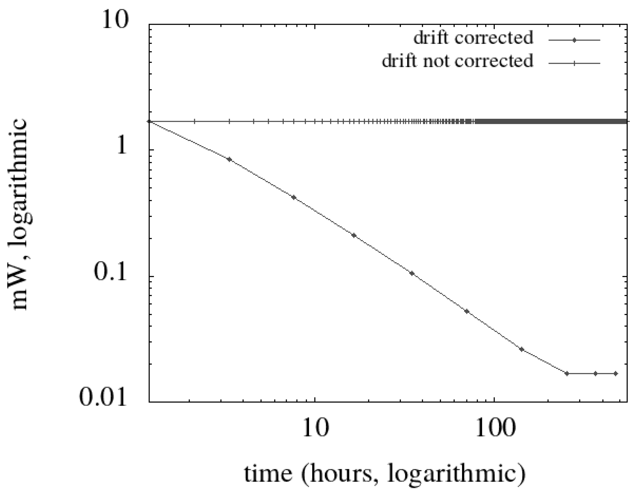
In Table 1, the numerical unfolding of a case study is shown. We envision a WiFi mote that can obtain from a time server an estimate of the proper time with an uncertainty of 0.1 s. As a requirement, the uncertainty of SDCk timestamps in the mote must be lower than 0.5 s, which is consistent with Equation (18). The values of (100 ppm) and (1 ppm) are nearly those expected from a quartz clock, comparable with those found by Rantwijk [9]. The energy required by a synchronization event is computed considering that the IoT device needs to turn on the WiFi interface, join the Access Point, perform a message exchange, and process the data. Using experimental results [10], we consider a duration of 15 s for this operation, during which the WiFi interface, normally in standby, requires an additional 150 at 3 . Intensity and voltage are coarse approximations derived from datasheets, and confirmed by measurement with a digital multimeter. With such values, the energy needed by one synchronization event () is 6.75 . Given such operational parameters, the mote should reach the floor value after 10 days, with seven synchronization events (see Figure 1). At that time, power consumption stabilizes at W, with a synchronization event every 4.6 days.
In Figure 1, we show the resulting time/power diagram compared with that obtained without drift correction: we observe that we obtain an improvement of one order of magnitude after one day of operation, which stabilizes at two orders of magnitude after ten days.
4. An Algorithm for the Optimal Scheduling of Synchronization Events
The scheduling algorithm controls the timing of clock synchronization events. Each component uses the results to implement the SDCk, and to schedule the next synchronization event: Algorithm 1 formally defines the program, while the rest of this section is an extended comment of it.
| Algorithm 1 The clock synchronization algorithm. The abstract function implements the synchronization event. The time function implements the SDCk, and returns a timestamp. The abstract function returns the value of the hardware clock. The function waits for a given amount of time (measured on the hardware clock) |
| 1: function timestamp 2: return 3: end function 4: while true do 5: 6: if defined(t’) then 7: 8: else 9: [ 10: end if 11: 12: 13: 14: end while |
After each synchronization event (represented by the abstract function in the program, in line 5), the device computes the estimated value of and that of the uncertainty , using respectively Equation (15) and Equation (16) (in line 7). The computation depends on the values in the previous round, and the initial values are used during the first round (line 9).
The value of is used to schedule the optimal timing for the next synchronization event, using Equation (17) (line 11).
The value of , together with t and from the returned triple, are used to define the logical clock function, according to Equation (6) (line 11).
At the end of each round, the triple from the previous synchronization is replaced with the current one (line 12), and the program is suspended until it is time for another synchronization event (line 13).
5. Hardware Matters
IoT devices are designed with an eye to power saving, and exhibit hardware features that need to be taken into account in software design. This section gives an overview of hardware-related aspects that have an impact on clock synchronization.
A hardware clock is often implemented using a counter driven by an oscillator. The counting register has a defined capacity and a pulse is produced every time an overflow occurs. Such a low frequency pulse produces an interrupt that software uses as the hardware clock tick. Hardware clock ticks are counted in their turn, and the counter value represents the hardware time of the device.
The oscillator tolerance depends on technology, and the deviation of its frequency from the nominal one is represented, in our model, as (see Equation (2)). The critical component in the oscillator is the resonator, a passive electronic component that determines the frequency. Various technologies are used to make such component, which may be manufactured with different degrees of precision. Depending on that, the frequency may dynamically change in a wider range, and the real frequency may differ more or less from the nominal one. In the previous section, we have shown how such aspects have an impact on power consumption.
The clock counter has a limited capacity, the maximum number that can be represented. This value, together with the frequency with which it is incremented, limits the maximum time interval that can be measured. When such a maximum value is reached, the counter overflows, and restarts its count from 0: this event is commonly called clock overrun. Using an unsigned variable, it is possible to tolerate a single overrun in a measured period of time. In our case, this limits the length of the interval between two successive synchronization events.
For instance, consider a clock counter with the capacity of 32 bits with a 1 clock period. We have an overrun after ms, less than 50 days. The use case of Table 1, for which the limit value for the interval between synchronization events is of a few days, exhibits a single overrun every circa 10 periods, and therefore it is not affected by such a limit if equipped with a 32-bit processor. Counting the number of overrun events is indeed possible, but hits against the limited computational capacity of the system.
Another relationship between clock synchronization and low power requirements is connected with power-saving features of the MCU (the MicroController Unit). In order to reduce power consumption, such devices offer various power-saving operation modes, which allow for switching off power-consuming functions of the processor for a given period of time.
Not only the on-board network device can be suspended, which is the rationale for this work, but also some CPU functions. If this option is considered, it becomes appealing to switch off the hardware clock, whose operation requires most of processor capabilities. When this is the case, the duration of sleep periods contributes to the offset of the SDCk with respect to the proper time, and must be exactly recorded in the offset of the clock (see Equation (6)). This fact has two relevant effects:
- the rollover period of the clock counter is significantly increased, but the problem shifts on the offset ;
- uncertainty in the time spent in a suspended state affects the SDCk uncertainty. Unfortunately, the hardware clock used to timeout the suspend state introduces a relevant uncertainty.
To conclude this section devoted to hardware related problems, we remark that the software that implements the SDCk should have a footprint compatible with the limited computational capabilities of the MCU, taking into account that the SDCk cannot take up more than a small fraction of the available capacity to leave room for IoT applications.
6. Proof of Concept—Implementation and Discussion
The proof of concept aims to observe the progressive convergence of the clock drift estimate to a value, and the corresponding decrement of drift uncertainty . To understand the limits of the algorithm, we will push the operation beyond the drift calibration limit represented by . In this way, we find that the resonators of the two sample devices (that are undocumented low-cost clones) have a different technology, and that different thresholds are appropriate. When a reasonable is found, we are able to quantify and discuss the power consumption for clock synchronization on the two devices. In a design oriented to production, the should be derived from board specifications, while in our case we find it by experiment.
To explore a practical application of our results, the platform for the proof of concept exhibits interesting constraints due to hardware devices with limited computing capabilities, and by a communication infrastructure with non-deterministic delays: the MCU is an Arduino board, the networking infrastructure is WiFi, the clock synchronization protocol is ntp.
6.1. The Network Synchronization Protocol
Until this point, our investigation has been agnostic of the way in which the synchronization event is performed, as long as the device participating to such an event returns the triple . Among the many technologies that can be used to implement a synchronization event, we mention the GPS service, long-wave radio broadcasts, broadband networks, and also the Internet standard NTP.
ntp is universally used for synchronization over the Internet. Its time resolution is (less than 1 ), well above our needs. To achieve it, the protocol adopts a time representation format (seconds and fractions are 32-bit numbers in fixed point notation) that needs conversion and rounding in order to be processed by the Arduino. This affects program complexity to the point that we preferred to write ad hoc code for our experiments, instead of using the existing library which is more complete but with a relevant footprint.
The ntp communication pattern is very simple, consisting of a two-way request/response protocol between a client and a server. The response contains three timestamps generated by the server reading its hardware clock: one associated with the last ntp synchronization event run with an higher level server, another with the receive operation of client request, and the third one with the send of the response. Only the last one is of interest for us.
The i-th synchronization event is performed using the data from the ntp roundtrip, as described in Equation (8). The client computes the following data, using its hardware clock as a time reference:
- is half the delay between sending the request to receiving of response (aka roundtrip time);
- is the hardware clock when the ntp request is sent augmented by half ;
- is the difference between the server timestamp when the request is received (found in the ntp response), and the time .
6.2. Hardware Platform
Our benchmark uses Arduino for the MCU, a ESP-01 board from Espressif (Shangai, China) as network interface, a WiFi network for its connection to the Internet. The schema is available at https://hackaday.io/project/107721-a-protoshield-as-a-wifi-shield. The ntp client is implemented on the Arduino with ad hoc code available at https://create.arduino.cc/editor/mastroGeppetto/6c681e2c-c316-43f7-8f97-a866a82c22af/preview, the server is a public stratum-1 ntp server, probably driven by an atomic clock.
To explore the behavior of the algorithm described in Section 4, we run the same code on two different boards, both belonging to the Arduino family and thus sharing the same MCU but using different clock technologies. As we will see, the results are very different in the two cases, and reveal the presence of a quartz clock on one board, and a ceramic resonator on the other: a difference that has a significant impact on energy consumption.
6.3. The Experiments
Each experiment consists of a series of synchronization events controlled by Algorithm 1; the same experiment is carried out on both hardware prototypes, and, depending on results, may last days.
Algorithm operation is controlled by the constants listed in the top box of Table 2. Let us see how we defined their values for our experiments.
To give a consistent value for the uncertainty limit , we need first a value for the uncertainty of the clock synchronization event. An estimate of it may be obtained from the roundtrip between the MCU to the ntp server. A lower bound for is then obtained as three times the value of , as from Equation (18). In our case, we estimated a worst-case roundtrip time of , which entails an of . The maximum uncertainty was then set as , in excess of 33 from the minimum.
To find an initial value for and , we use the data available for ceramic resonators [11]. Since drift uncertainty (i.e., frequency tolerance) for these kinds of devices is around and above 1000 ppm, we use this value for , while the initial drift is set to 0, meaning that the uncertainty range for the hardware clock frequency is centered on the nominal frequency, and its width corresponds to frequency tolerance. With such initial values, the interval between the first two synchronization events is 154 s long, and would remain such if the drift were not corrected.
The energy requirements for each synchronization event () are those already discussed for the use case. Such initial conditions (summarized in Table 2) are used for all experiments. Environment conditions are similar as well: the temperature has been monitored, and varies between 23 and 28 .
For our experiments, we set , since we want to find a good value for it. We expect that the limit uncertainty is violated when the value of falls under . To detect this event, just after each synchronization event , the new estimate of the proper time is matched against the timestamp provided by the SDCk, by computing the difference between the two as
If the difference between the two is less than the maximum uncertainty , we conclude that the uncertainty limit is valid, since
Instead, if Equation (23) does not hold, we conclude that the requirement has been violated because we exceeded the limit value for .
6.4. Experimental Results and Discussion
We run a total of three experiments: two of them with an unbranded undocumented clone of the Arduino Pro Mini, another with a branded but equally undocumented clone of the Arduino Uno. Both boards use the same MCU, an ATmega328p from Atmel (San Jose, CA, USA), but different accessory hardware, included the resonator.
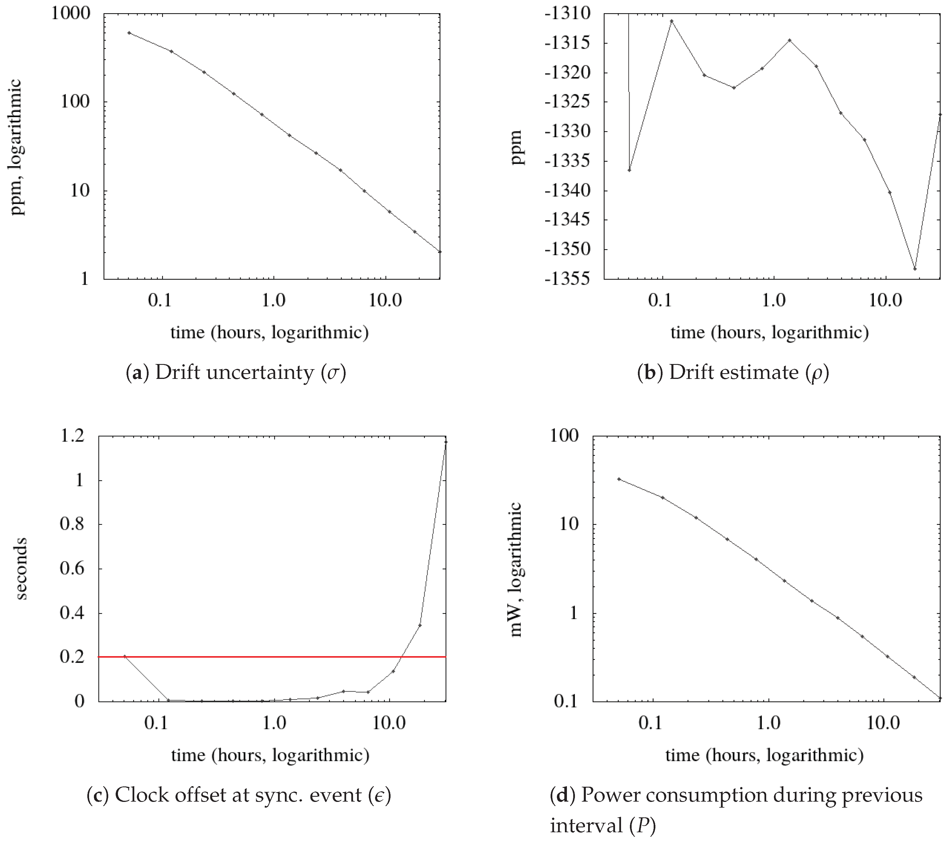
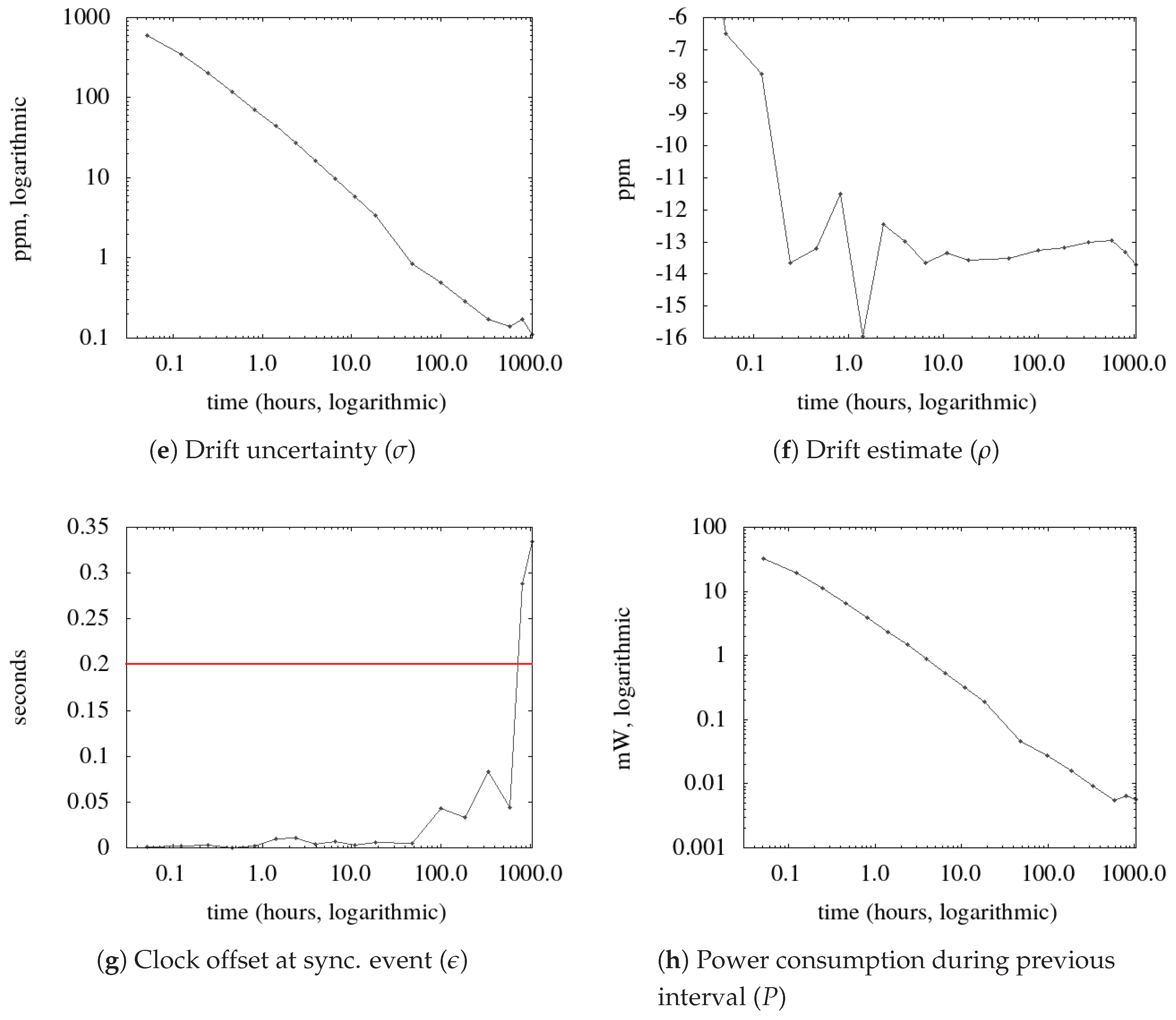
The results are summarized in three figures, one for each experiment (see Figure 2, Figure 3 and Figure 4), each containing four diagrams. A dot in the diagrams represent values associated with a synchronization event. All diagrams have an identical logarithmic time scale in hours, so that equally spaced points correspond to exponentially growing time intervals. (Diagram a) shows how drift uncertainty () decreases during the process. At the beginning of the process, this value corresponds to the nominal tolerance of the resonator, in ppm. After every synchronization event, the uncertainty decreases exponentially. (Diagram b) shows the drift estimate computed after each synchronization event (): it tends to stay around the real value of drift, but it is affected by uncertainties in the synchronization event and by drift variations. This value is used to compute the timestamps produced by the SDCk. (Diagram c) shows the difference between the timestamp produced by the SDCk and that received from the NTP server. It is a benchmark parameter, since it must remain below the expected uncertainty, marked by a red horizontal line. (Diagram d) shows the power consumed during the last period between synchronization events: it contributes to the overall power defined in (21). The y-axis has a logarithmic scale in order to display a wide range of values.
Regarding the Arduino Pro Mini, one experiment aims at finding a value for , another to check the operation when such a value is used. The results of the first experiment are shown in Figure 2. In diagram c, the value of Equation (23) is shown, and the horizontal line marks the threshold uncertainty . After eight hours, the computed value exceeds the threshold, indicating a failure of the SDCk. We ascribe this to the absence of a valid value for , which was set to 0. Thus, we record the last value of before the violation, and we assume that value as a lower bound for . It falls around 8 ppm, and might depend on environmental conditions, like temperature variations. Diagram d shows that power consumption continues to drop exponentially, but this result is not meaningful after the SDCk violates its requirements.
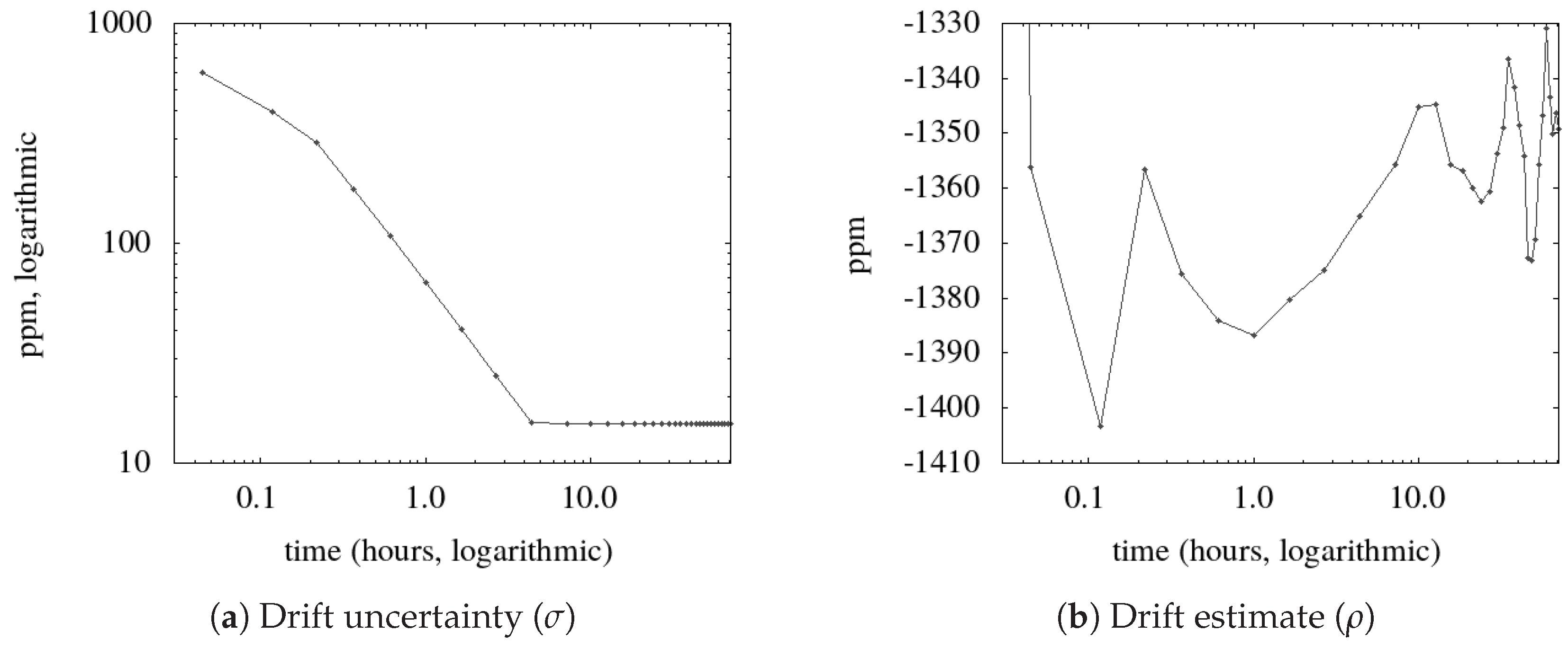
In the next experiment, we use the same board with ppm, which doubles the lower bound found in the previous experiment. The results (see Figure 3) prove that with this configuration the bound uncertainty requirement remains valid (frame c) for the duration of the experiment (more than four days), but, in the long run, a synchronization event is needed every circa three hours, while drift estimate (in diagram b) oscillates in the range .
Such a drift is unexpectedly high (circa five seconds per hour), and falls outside the configured initial range . The limited consequence of this configuration error is that, during the first three minutes of operation, the timestamp provided by the SDCk falls outside the required range (in diagram c). However, the divergence is promptly corrected, and, during the following four days of operation, the timestamps fall within the required range.
From the two experiments, we conclude that both the drift and its uncertainty are consistent with those of ceramic resonators, a low-cost alternative of crystal-based ones.
Power consumption (see diagram d) stabilizes when the floor value for is reached; we discuss this value after the analysis of the next experiment.
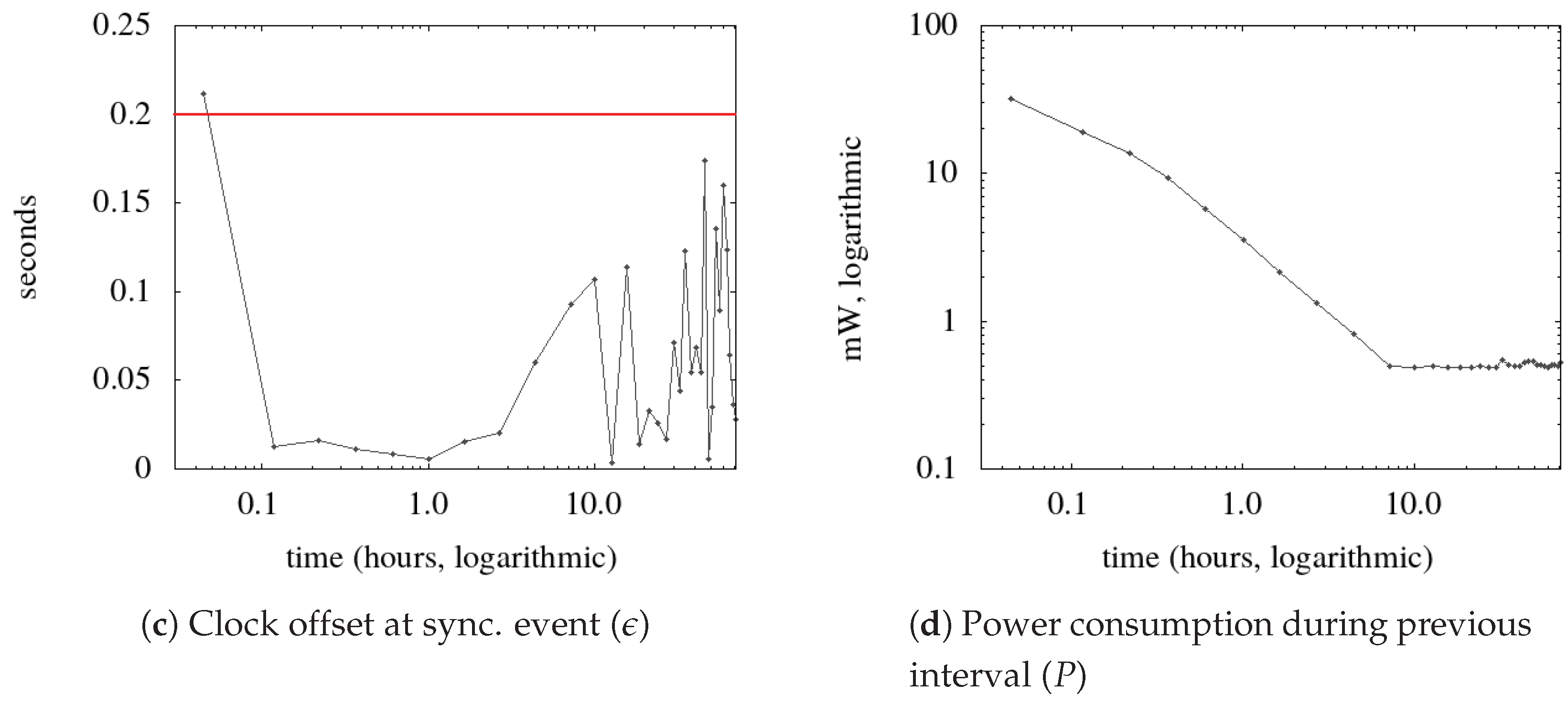
The third experiment uses an Arduino Uno clone, and lasts over one month. The threshold is violated after 23 days of operation (see Figure 4). This occurs when the goes below ppm, which is therefore considered a lower bound for the of this board. Using such value the period between synchronization events is longer than ten days (254 h), which favorably compares with the three hours of the ceramic oscillator.
The estimated drift of the resonator (see Figure 4b) is centered at ppm, one second per day, which is consistent with typical quartz characteristics [12]; such resonators feature a superior stability and frequency tolerance compared with ceramic ones. However, clock stability looks significantly better than that one might expect from a quartz crystal, whose frequency variation is usually on the order of ppm for each temperature degree.
To compare the power consumption of the two devices, we refer to the results shown in Figure 3d and Figure 4d. The latter (Arduino Uno with quartz clock) drops below , the former (MiniPro with ceramic resonator) stays around , both controlled by an appropriate value for . The advantages of a stable resonator are evident, since we obtain a power rate of more than 50 times in favor of the quartz driven device.
As a final remark, power consumption without drift correction would be stable to the value corresponding to a drift uncertainty of 1000 ppm, which means 45 with one synchronization event every 154 s.
7. Related Works
Clock synchronization is a fundamental topic in distributed computing, with a substantial number of papers that provide smart approaches and solutions. Indeed, most of the literature covers the underlying communication protocol, which we call a synchronization event, like Wang et al. [13] that propose to introduce time information in level 2 (MAC) communication. There is a wide literature regarding protocol specific solutions for clock synchronization: limiting to applications that are close to the topic of this paper, Sundararaman et al. [14] give an exhaustive survey dated April 2005.
Our paper abstracts from the implementation of the synchronization event, be it master-slave or peer-to-peer, internal vs. external, single or multi-hop, to cite some of the categories used in the referenced survey [14]; instead, we focus on how to use the information received by way of that event. Besides using its results to synchronize its SDCk, we show how to obtain a substantial power saving by measuring and correcting the hardware clock drift. Notably, the term drift is used in diverse ways in the literature; we use it to indicate the clock frequency offset, the difference from the nominal and the real value of this parameter. To cite one, in the referenced survey [14], the term skew is used instead of drift.
Drift calibration is often obtained in hardware, for instance with an adjustable capacitor, but this solution is impractical for massive low-cost production, since each device should be individually tuned, and for this reason a software approach is preferable. However, clock drift correction is seldom considered in software-oriented papers, or treated as marginal, as an add-on for a clock synchronization protocol. For instance, in the paper describing the Flooding Time Synchronization Protocol (FTSP [15]), the authors dedicate a section to the estimate of the drift of a Mica2 mote, but this result is not used in the protocol. Maróti et al. [16] analyze and measure the clock drift of the nodes in a cluster of ASUS motherboards, with results that are not related with IoT systems but nevertheless useful to frame the problem.
A paper by Wu et al. [17] is a relevant representative of papers that aim at estimating clock parameters, offset and drift, using statistical methods. They apply data fusion algorithms specifically designed for wireless line of sight networks from a collection of clock synchronization events. Such data are filtered using signal processing techniques in order to obtain the values of interest. Their approach is very different from ours: in the first place, they consider clock parameters as constant data, while we demonstrate that real limits arise from the variable component of the drift. To introduce statistical signal processing techniques, the authors use a probabilistic model for the system, while we prefer a non-deterministic model that avoids problems related with long-tail phenomena in clock synchronization events, which emerge in routed, multi-hop networks.
Meier et al. [18] introduce a sender-receiver clock synchronization protocol, using the drift-constraint clock model, which corresponds to the one used in this paper. They also prefer, as we do, the term uncertainty in time measurement, instead of the commonly used error. Like the authors of the former paper [17], they do not consider clock synchronization as a dynamic process, the timing of which may be determined by the results of the process itself, and they overlook the power consumption issue.
A power-aware attitude is found in a paper by Chaudhari et al. [19] that shows how, in broadcast networks (wireless, in their case), a component can obtain a significant power saving by eavesdropping synchronization events requested by others: only one component pays the energy to transmit the request packet, but many take advantage of the event, a feature exploited also by FTSP [15]. In this case, our assumption that all events require an identical energy falls, so the model should be adapted to be suitable for this case. Our dynamic approach to drift correction is still applicable, but the energy trend differs in the details.
Recent results on the subject are found in a paper by Mani et al. [20] that aims at clock synchronization in a system of heterogeneous devices. This is a study that comes to experimental results and to conclusions that are consistent with ours, concerning the quality of clocks of IoT devices. One section is devoted to rate synchronization, which corresponds to drift estimate in our protocol. In a sense, their conclusions are the starting point for our paper, since they conclude that synchronization intervals are longer for stable clocks, and that this fact is relevant for protocol optimization. Their experimental results demonstrate that synchronization intervals may be dynamically adjusted, which is the topic that we investigate in our paper.
Taking the latter paper as a touchstone, we remark that our formal model is exhaustive and provides useful rules of thumb for the designer, while Mani et al. simply introduce an algorithm description. Our work is not targeted to a specific clock synchronization protocol, while Mani et al. embed their algorithm in a wider design. Our experimental results favorably compare with those documented in the referenced paper, where the power required by the clock synchronization process is not considered.
8. Conclusions
The management of a system is simplified if its components share the same time reference. For instance, activities can be scheduled in advance without further communication, and local events are ordered using global timestamps. To this end, the components may implement software-defined clocks, and keep them in pace with synchronization events. In a network of sensors, it is important to find a compromise between simplicity and power consumption, and this paper introduces a simple strategy to reduce power consumption.
In order to find results that are widely applicable, we define a model that abstracts from the internals of the synchronization event. The model is non-deterministic, and it does not introduce assumptions on a probabilistic nature of events. Instead, it quantifies an uncertainty that characterizes measurements and observations. Using such a formal framework, we find that hardware clock stability has a direct impact on the power needed to keep clocks synchronized, and that, depending on its stability, the clock drift can be gradually corrected in the software defined clock. Under simply stated and not overly restrictive conditions, this result can be obtained with a simple algorithm.
We demonstrate its soundness with a real world proof of concept, where an Arduino implements a software defined clock that is synchronized using NTP, and we discuss the results. The experiments are reproducible, since device schematics and the Arduino sketch are available on public repositories.
The results of our investigation are readily applicable, but are limited to the constant component of the hardware clock drift. To further reduce power consumption, we envision a model that includes frequency/temperature dependency, which is the first source of drift variability.
Supplementary Materials
The following are available at https://www.mdpi.com/2224-2708/8/1/11/s1. The Addenda.zip archive bundled to this paper contains material intended to help those that want to reproduce or improve the results presented here. It should not be used for deployment and operation, although part of it have been successfully deployed in real scale experiments.
The archive includes the following files and directories:
- model.gnumeric: a simulator and a computer used to produce Figure 1 and for computations based on the abstract model. Uses gnumeric application (http://www.gnumeric.org/)
- 20180718_MiniPro.csv: the data used for Figure 2
- 20180816_MiniPro_sigma15.csv: the data used for Figure 3
- 20180720_ArduinoUno_new.csv: the data used for Figure 4
- NTP_sync: the Arduino sketch used for the experiments, with an embedded library. Uses Arduino IDE (https://www.arduino.cc/). Note that the library is available separately (subject to upgrade) on https://bitbucket.org/augusto_ciuffoletti/atlib.
- TestMote.fzz: the schematics of the test mote. Uses Fritzing application (http://fritzing.org/).
The links to the sketch and to the schematics that are included in the paper make reference to items recorded in public domain repositories, that might be upgraded in the future.
Funding
This research received no external funding.
Conflicts of Interest
The author declares no conflicts of interest.
References
- Lamport, L. Time, Clocks, and the Ordering of Events in a Distributed System. Commun. ACM 1978, 21, 558–565. [Google Scholar] [CrossRef]
- Sun, C.; Jia, X.; Zhang, Y.; Yang, Y.; Chen, D. Achieving Convergence, Causality Preservation, and Intention Preservation in Real-time Cooperative Editing Systems. ACM Trans. Comput. Hum. Interact. 1998, 5, 63–108. [Google Scholar] [CrossRef]
- Bernstein, P.; Shipman, D.; Wong, W. Formal aspects of serializability in database concurrency control. IEEE Trans. Softw. Eng. 1979, 5, 203–216. [Google Scholar] [CrossRef]
- Swan, M. (Ed.) Blockchain—Blueprint for a New Economy; O’Reilly Media: Sebastopol, CA, USA, 2015. [Google Scholar]
- Mills, D. Network Time Protocol (Version 3); Request for Comment 1305; IETF, Network Working Group: Fremont, CA, USA, 1992. [Google Scholar]
- Rowe, A.; Gupta, V.; Rajkumar, R.R. Low-power Clock Synchronization Using Electromagnetic Energy Radiating from AC Power Lines. In Proceedings of the 7th ACM Conference on Embedded Networked Sensor Systems, SenSys ’09, Berkeley, CA, USA, 4–6 November 2009; ACM: New York, NY, USA, 2009; pp. 211–224. [Google Scholar] [CrossRef]
- Cristian, F. Probabilistic clock synchronization. Distrib. Comput. 1989, 3, 146–158. [Google Scholar] [CrossRef]
- Ciuffoletti, A. Sharing a common time reference in a heterogeneous distributed system. In Proceedings of the 7th EUROMICRO Workshop on Parallel and Distributed Processing, Funchal, Portugal, 3–5 February 1999; pp. 359–366. [Google Scholar] [CrossRef]
- van Rantwijk, J. Available online: http://jorisvr.nl/article/arduino-frequency (accessed on 15 January 2019).
- Ciuffoletti, A. Design and implementation of a low-cost modular sensor. In Proceedings of the 13th IEEE International conference on Wireless and Mobile Computing (WiMob), Rome, Italy, 9–11 October 2017. [Google Scholar]
- Murata Manufacturing Co., Ltd. Ceramic Resonators. Available online: http://www.farnell.com/datasheets/1506176.pdf (accessed on 15 August 2018).
- Murata Manufacturing Co., Ltd. Crystal Unit. Available online: http://www.farnell.com/datasheets/321153.pdf (accessed on 15 August 2018).
- Wang, H.; Zeng, H.; Wang, P. Clock Skew Estimation of Listening Nodes with Clock Correction upon Every Synchronization in Wireless Sensor Networks. IEEE Signal Process. Lett. 2015, 22, 2440–2444. [Google Scholar] [CrossRef]
- Sundararaman, B.; Buy, U.; Kshemkalyani, A.D. Clock synchronization for wireless sensor networks: A survey. Ad Hoc Netw. 2005, 3, 281–323. [Google Scholar] [CrossRef]
- Maróti, M.; Kusy, B.; Simon, G.; Lédeczi, A. The Flooding Time Synchronization Protocol. In Proceedings of the 2nd International Conference on Embedded Networked Sensor Systems, SenSys’04, Baltimore, MD, USA, 3–5 November 2004; ACM: New York, NY, USA, 2004; pp. 39–49. [Google Scholar] [CrossRef]
- Marouani, H.; Dagenais, M.R. Internal Clock Drift Estimation in Computer Clusters. J. Comp. Sys. Netw. Commun. 2008, 2008, 9. [Google Scholar] [CrossRef]
- Wu, Y.; Chaudhari, Q.; Serpedin, E. Clock Synchronization of Wireless Sensor Networks. IEEE Signal Process. Mag. 2011, 28, 124–138. [Google Scholar] [CrossRef]
- Meier, L.; Blum, P.; Thiele, L. Internal Synchronization of Drift-constraint Clocks in Ad-hoc Sensor Networks. In Proceedings of the 5th ACM International Symposium on Mobile Ad Hoc Networking and Computing, MobiHoc’04, Tokyo, Japan, 24–26 May 2004; ACM: New York, NY, USA, 2004; pp. 90–97. [Google Scholar] [CrossRef]
- Chaudhari, Q.M.; Serpedin, E.; Kim, J. Energy-Efficient Estimation of Clock Offset for Inactive Nodes in Wireless Sensor Networks. IEEE Trans. Inf. Theory 2010, 56, 582–596. [Google Scholar] [CrossRef]
- Mani, S.K.; Durairajam, R.; Barford, P.; Sommers, J.C.U. A System for Clock Synchronization in an Internet of Things. arXiv, 2018; arXiv:1806.02474. [Google Scholar]
Figure 1.
Comparison of the theoretical trend of power consumption during each period of the synchronization process, with and without drift correction. Each mark corresponds to a synchronization event. Operational parameters are in Table 1. If drift is corrected (lower line), power consumption drops exponentially since the interval between synchronization events grows exponentially. The decreasing trend stops when the threshold drift uncertainty is reached. If drift is not corrected power consumption remains constant.

Figure 2.
Results of the first experiment with an undocumented clone of the Arduino Pro Mini. Clock uncertainty (c) diverges and exceeds the threshold (in red), after (8 h). The reason is that drift variation (b) during such periods exceeds drift uncertainty (a), which is higher than 10 ppm because of clock instability.

Figure 3.
Results of the second experiment with an undocumented clone of the Arduino Pro Mini. To avoid the divergence shown in Figure 2, a 15 ppm floor threshold has been introduced for drift uncertainty. Clock uncertainty (a) remains within the limits during the entire duration of the experiment (55 h). Power consumption (d) stabilizes around .


Figure 4.
Results of the experiment using an undocumented branded clone of the Arduino Uno. Clock uncertainty (c) diverges and exceeds the threshold (in red), after 590 h (24 days). The reason is that drift variation (b) during such periods exceeds drift uncertainty (a), around ppm because of clock instability. We conclude that a threshold ppm is a lower bound of drift uncertainty for this board, with an associated power consumption (d) of .


Table 1.
Operational parameters for a use case: on top the values from the use case specifications, below the expected performance. Use case specifications are appropriate for a quartz crystal resonator with a wide frequency tolerance.
Table 1.
Operational parameters for a use case: on top the values from the use case specifications, below the expected performance. Use case specifications are appropriate for a quartz crystal resonator with a wide frequency tolerance.
| Use Case Specifications | |
| 100 ppm | |
| 1 ppm | |
| × 3 × 15 (= ) | |
| Results after Convergence at | |
| P | |
| d (= ) | |
Table 2.
Initial values and constants for the experiments.
| 1000 ppm | |
| 0 ppm | |
| to be found, see paper | |
© 2019 by the author. Licensee MDPI, Basel, Switzerland. This article is an open access article distributed under the terms and conditions of the Creative Commons Attribution (CC BY) license (http://creativecommons.org/licenses/by/4.0/).
Share and Cite
MDPI and ACS Style
Ciuffoletti, A. Power-Aware Synchronization of a Software Defined Clock. J. Sens. Actuator Netw. 2019, 8, 11. https://doi.org/10.3390/jsan8010011
AMA Style
Ciuffoletti A. Power-Aware Synchronization of a Software Defined Clock. Journal of Sensor and Actuator Networks. 2019; 8(1):11. https://doi.org/10.3390/jsan8010011
Chicago/Turabian StyleCiuffoletti, Augusto. 2019. "Power-Aware Synchronization of a Software Defined Clock" Journal of Sensor and Actuator Networks 8, no. 1: 11. https://doi.org/10.3390/jsan8010011
Note that from the first issue of 2016, this journal uses article numbers instead of page numbers. See further details here.