Article

Method for the Analysis and Visualization of Similar Flow Hotspot Patterns between Different Regional Groups

1
Key Laboratory of Virtual Geographic Environment, Ministry of Education, Nanjing Normal University, Nanjing 210023; China
2
State Key Laboratory Cultivation Base of Geographical Environment Evolution (Jiangsu Province), Nanjing 210023, China
3
Jiangsu Center for Collaborative Innovation in Geographical Information Resource Development and Application, Nanjing 210023, China
4
School of Computer Science and Technology, Nanjing Normal University, Nanjing 210023, China
5
Department of Geography Sciences, University of Maryland College Park, MD 20742, USA
6
School of Geographic and Biologic Information, Nanjing University of Posts and Telecommunications, Nanjing 210023, China
*
Author to whom correspondence should be addressed.
These authors equally contributed to the work.
ISPRS Int. J. Geo-Inf. 2018, 7(8), 328; https://doi.org/10.3390/ijgi7080328
Submission received: 30 June 2018 / Revised: 1 August 2018 / Accepted: 13 August 2018 / Published: 15 August 2018

Abstract

:
Interaction among different regions can be illustrated in the form of a stream. For example, the interaction between the flows of people and information among different regions can reflect city network structures, as well as city functions and interconnections. The popularization of big data has facilitated the acquisition of flow data for various types of individuals. The application of the regional interaction model, which is based on the summary level of individual flow data mining, is currently a hot research topic. Thus far, however, previous research on spatial interaction methods has mainly focused on point-to-point and area-to-area interaction patterns, and investigations on the patterns of interaction hotspots between two regional groups with predefined neighborhood relationships, that being with two regions, remain scarce. In this study, a method for the identification of similar interaction hotspot patterns between two regional groups is proposed, and geo-information Tupu methods are applied to visualize interaction patterns. China’s air traffic flow data are used as an example to illustrate the performance of the proposed method to identify and analyze interaction hotspot patterns between regional groups with adjoining relationships across China. Research results indicate that the proposed method efficiently identifies the patterns of interaction flow hotspots between regional groups. Moreover, it can be applied to analyze any flow space in the excavation of the patterns of regional group interaction hotspots.

1. Introduction

Our society is built on the basis of mobility of certain elements, such as people, goods, and information technology. These flow elements form a flow space [1]. In contrast to the traditional local space, flow space emphasizes the interaction and interactive relationships of elements [2,3]. Geographers used to focus on physical space [4,5,6] but have turned their attention to flow space because of the continuous advancement of economic globalization and Internet technology [7,8,9,10]. Drastic changes in the global economy have strengthened global exchanges through tourism, trade, and technology, thereby directly promoting the flow of people, logistics, and technology. In addition, with the development of Internet technology, information flow has decreased distances between places [2]. Distance is no longer an applicable metric of space when the time required to transmit information over one kilometer is almost the same as that required to transmit information over 100,000 kilometers. That is, the Internet has changed the transmission of spatial information. In fact, geographers should focus not only on the flow space itself, but also on the reconstruction of spatial organization structure based on flow elements, the function of organization networks, and the identification of emerging flow patterns [11]. Therefore, a quantitative analytical method for establishing and defining interaction patterns is important because they are the base methods for defining spatial relationships between two regional groups.
Many methods for determining the interaction patterns of flow space have been proposed over the past few decades. Numerous algorithms used to mine comprehensive spatio-temporal interaction patterns for spatial interaction models have been constructed [12,13,14,15,16]. However, the spatial dependence of interactive nodes in these methods is limited. Some of these nodes apply complex network methods to discover spatial interaction patterns [17,18,19,20]. Models for regional interaction based on the concept of complex networks have been proposed [21]. These models, such as the method of interaction relation proposed by Kira, consider dependencies and similarities among flowing nodes to identify areas with strong interactivity. However, this method only recognizes individual regions with similar interactions rather than interaction patterns between different regions groups. A regional movement pattern recognition (MZP) algorithm based on the aggregation of metro nodes has been proposed [22]. Chen et al. expanded the proximity relationship on the basis of the MZP algorithm and taxi OD data and proposed the MPFZ algorithm [23]. All these methods mainly focus on point data and their adjacency relationship. Their main disadvantages are their inefficiency and inability to provide a visually well-resolved solution for the excavation of the interaction model, which enable to simultaneously visualize both analysis results and test parameters in a map. Thus, none of the aforementioned methods can provide a visual representation of the interaction pattern between two regional groups.
A basic characteristic of existing models is that they lack a recognition method for interactive flow patterns that may exist between one regional group and another. Moreover, the use of existing models to define adjacency relationships between two regional groups is difficult. We refer to the literature on adjacency matrixes to define regional adjacency relations. For example, strong interaction is not only observed between regions A and B (B does not have a predefined proximity relationship) but also in several of their surrounding regions. We assume that the interaction relationship is strong and that regions A and its surroundings and region B and its surroundings satisfy a predefined adjacency relationship. Then, regional groups A and B are located. Thus, we can conclude that a strong interaction between A or B and their surroundings exist. Moreover, a regional group interaction flow pattern is formed between regions A and B.
This work presents an advanced method for discovering, analyzing, and visualizing the flow patterns of interaction hotspots between two different regional groups. First, a review of literature is presented, and the expected results of the method is described (Section 2). Second, a new method, which is used to mine the flow patterns of regional groups, is proposed (Section 3). The regional adjacent relationship is defined (Section 3.1.1), the structure of the flow pattern mining algorithm is described (Section 3.1.2), and flow pattern visualization (Section 3.2.1) and methodological issues (Section 3.2.2) are introduced. Finally, a case study involving flow volume data and the proposed method is presented (Section 4).

2. Literature Review

Individual flow data are mainly modeled by the pattern of node-to-node flow [24,25]. Thus, many of the macro-pattern summary or interactive pattern discovery methods for individual flow data are based on node-flow data [26,27,28], and works on flow data modeling and analysis between regions remain limited. Moreover, interactions between areas can be abstracted as point-to-point interactions. Basic methods for spatial analysis can be easily used to model and analyze interactions between regional groups even if point-to-point flow data is aggregated to region-to-region flow data. However, interaction modeling and analysis between regional groups involve many issues, such as the identification, determination, and effective visualization of the regional adjacency relationship. Most of the existing works are based on the first two cases. Existing related research are briefly reviewed below. We discuss point-to-point and area-to-area flow patterns, as well as the flow patterns of two different regional groups, to understand the limitations of the objectives of existing methods. We specifically focus on patterns with strong relationships.
Most of the flow data exist in the form of point-to-point interactions with directional arrows. Related interaction analysis methods mainly include point-to-point interaction pattern mining [29,30,31,32,33] and interactive pattern mining in between multiple points, as well as the model analysis of adjacent points in the same community [34,35,36,37]. In Figure 1a, the interaction between the three nodes in the northwest corner and the two nodes in the southeast corner is remarkably stronger than that among the other nodes. A similar situation exists between the neighboring points in the southwest and northeast corners. Figure 1b illustrates that the MZP algorithm [22] can discover a strong interaction pattern between a set of adjacent nodes to another set of adjacent nodes in network-structure data. Then, the two patterns shown in Figure 1c could be identified. The MZP algorithm mainly solves such problems and provides valuable reference value for related research. However, this algorithm has extremely high time complexity and fails to provide a visual representation of analytical results. Thus, Chen et al. proposed the MPFZ method. However, Chen’s method only extended the data that had been applied by the network MZP algorithm from network node flow to other analyses of the arbitrary node flow data without implementing other major changes.
In some cases, the interaction pattern for flow data between different areas is emphasized. For example, the point-to-point with arrow data (Figure 2a) shows the area is obtained from area-to-area flow data through basic spatial overlay and statistical calculation methods. Figure 2a shows that the arrow must also contain an attribute to indicate the size of the interaction value for each area-to-area flow data. The results shown in Figure 2a indicate that the regional interaction shown on Figure 2b can be easily identified. Thus, the regional interaction pattern shown in Figure 2c is obtained.
The area-to-area model has an obvious disadvantage, that is, each area interaction pattern ignores the spatial autocorrelation characteristics of the starting and ending areas with other existing adjacent areas. Thus, any area interaction pattern and the surrounding area in interaction directions and sizes are autocorrelated. Figure 3a shows that the interaction between several adjacent areas in the northwest and southeast is more pronounced than those between the area-to-area flow data. Additionally, similar patterns are identified in the southwest and northeast sides. Figure 3b shows that the goal of this work is to identify the flow patterns of regional group interactions by defining specific area adjacency relationships. Figure 3c shows the results and visualization of the expected flow pattern. Then, further research on the interaction strength, value size, and significance level of each regional group must be conducted on the basis of analytical results. In this paper, a method for mining interaction patterns between regional groups is proposed, and a spatial interaction visualization solution similar to spatial or spatiotemporal [38] hotspots pattern visualization methods is also provided.

3. Methodology

In this work, the entire research framework includes the input of node-based flow data, the processing of data, and the interaction pattern mining, output, and visualization of regional group flow patterns (Figure 4). This study supports node-based flow data input during the design process because most of the flow data are counted and then stored by nodes. First, the input node-to-node flow data are converted in accordance with a certain regional unit and then converted into region-to-region flow data. This process can be realized by using common GIS overlay and statistics functions. Then, the adjacency relationship of the regional units is determined (Section 3.1.1), and adjacent areas wherein the interaction value reaches a certain threshold are merged on the basis of this adjacency relationship before being constructed into regional groups. Subsequently, all similar hotspot flow patterns between different regional groups are identified (Section 3.1.2). Finally, the geo-information Tupu visualization method is used to present regional groups with similar hotspot flow patterns, and visual variables are used to visualize the evaluation results of their own characteristics in each flow pattern. Hereafter, we refer to the similar patterns of flow hotspots between regional groups as RG-Flow-Pattern.

3.1. Algorithm for Similar Hotspot Patterns between Regional Groups

In this study, the algorithm for the modeling of regional interaction hotspots mainly includes three aspects, namely, (1) the definition of the regional neighborhood relationship, (2) the construction of an algorithm that reconstructs the patterns of regional interaction hotspots on the basis of defined neighborhood relationships, and (3) the use of multiple test parameters to evaluate the results of the identified area interaction hotspot models.

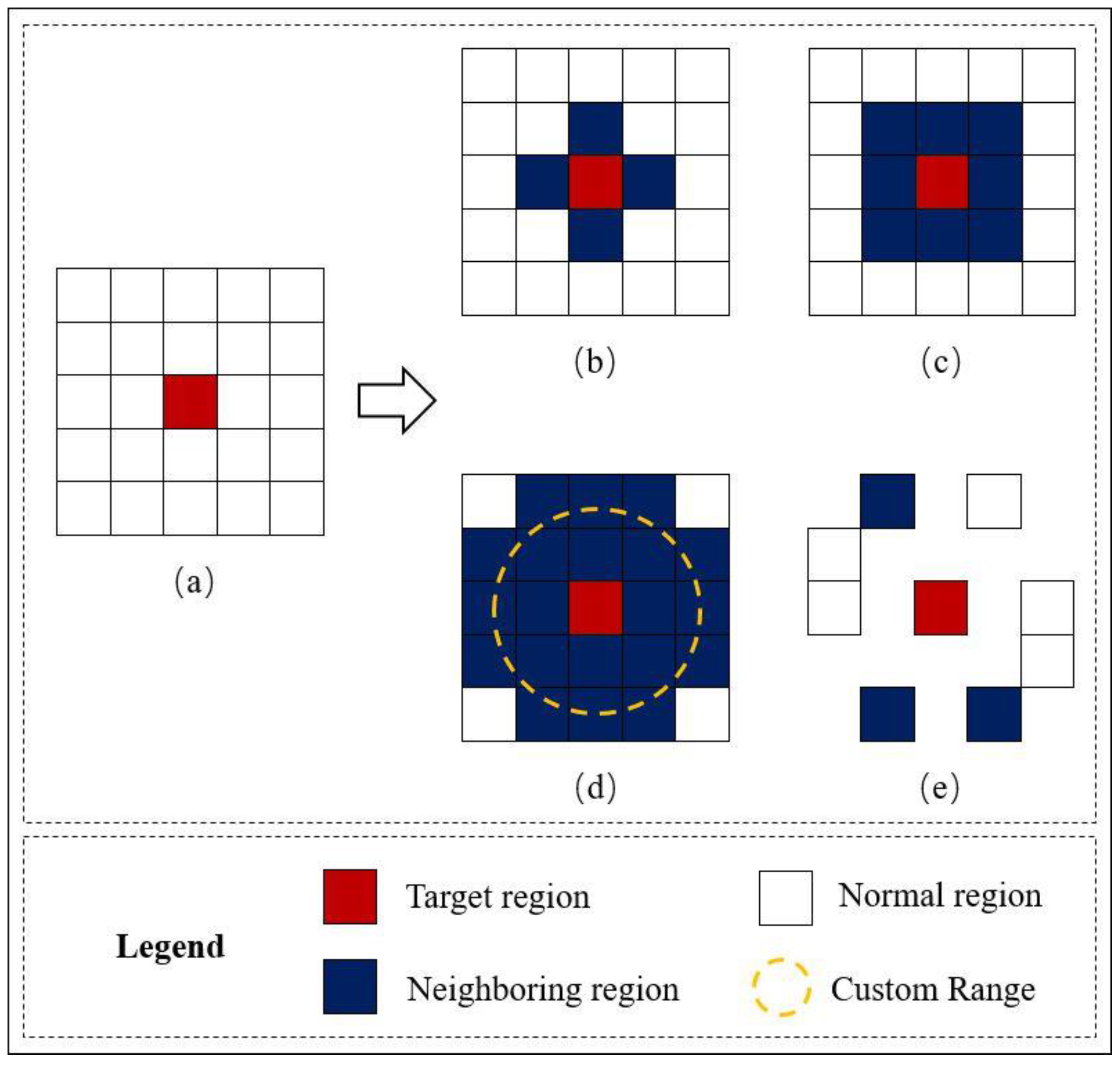
3.1.1. Regional Adjacency Relationship Modeling

We must define the regional adjacency relationship and its merger principle to identify the pattern of interaction hotspots. In the proposed method, four methods for determining the adjacency relationship of the area are defined. Figure 5 shows that if each grid is used as a region, then the adjacency relationship between regions can be expressed as that in Figure 5b–e. Figure 5a shows that if we assume that the target area is the red area, then the specific meanings of the four adjacency relationships can be briefly described as:
● Adjacent edges
In Figure 5b, four areas share common edges with the target area, and these four areas are defined as the adjacent areas of the target area. The adjoining relationship in this case is called an edge–adjacent relationship. Under this rule, a target area may have more or less than four adjacent areas in an actual partition.
● Adjacent edges and corners
Figure 5c shows an adjacency relationship similar to that shown in Figure 5b. However, it includes an area that shares a common node with the target area, except that the area with a common edge and a target area belongs to the adjacent edge of the target area. This kind of adjoining relationship is called edge–corner adjacency.
● Customized adjacent range
In Figure 5d, a circular buffer area is defined with the center of mass of the target area as the origin. When other areas are within or intersect the buffer area, they are defined as the adjacent areas of the target area. In this method, the adjacency relationship is called the adjoining relationship of customized adjacent range.
● Logical adjacent relationship
In addition to the three aforementioned methods used to define the adjacency relationship, we can also determine whether the target area and the other areas are adjacent by customizing the logical relationship that is independent of the spatial position. Figure 5e shows logical relations between the three blue areas and the target area. Therefore, although these three areas do not coincide with the target area or the vertices, they are defined as the adjacent areas of the target area.
Basically, these four approaches are the typical modeling methods used to present the spatial relationship of surface features. Other adjacencies include k-nearest and are custom based on the spatial adjacency matrix.

3.1.2. Region Merging and Recognition of Similar Hotspot Flow Patterns

● Definitions of similar hotspot flow patterns between regional groups
In this study, a set of datasets that contain n planar area units are given as Rset = { R 1 , R 2 , , R n } ( i = 1 ,   2 , , n ) , where R i represents the nth region. In a regional group interactive hotspot flow pattern, the origin area group is defined as R G O s e t = { R 1 , R 2 , , R u }, and the destination area group is defined as RGDset = { R 1 , R 2 , , R v }. In addition, regional flow is defined as the pair of origin and destination areas with interactions in a regional group interaction hotspot pattern. The dataset RFset is given to store all regional flow in the regional group interaction hotspot flow pattern, (RIH-FP); R F s e t = { R F 1 , R F 2 , , R F m } ( j = 1 ,   2 , , m ) . j th regional flow can be represented as R F j = R F j _ o R F j _ d , R F j _ o ϵ R G O s e t , indicating the origin of the regional flow. R F j _ d ϵ R G D s e t represents the destination area of regional flow. In some situations, for ease of exposition, we use the term flow pattern instead of RIH-FP. Flow pattern has various definitions.
Definition 1.
A regional group interactive hotspot flow model consists of three components, namely, the starting regional group RGOset, the destination regional group RGDset, and the interaction direction that indicates the interaction relationship. A regional group interaction hotspot pattern has the same direction as any R F j = R F j _ o R F j _ d in the RFset.
Definition 2.
A single region in the RGOset of the origin region group and in the destination region group RGDset must satisfy the definition of area-adjacent relationship given in Section 3.1.1.
Definition 3.
The number of regions in the origin and destination regional groups of a regional group interactive hotspot flow pattern cannot be 1 at the same time, that is, at least more than one region is included in the beginning or termination regional group.
Definition 4.
The interaction value of regional flow refers to the value of interaction from one region to another and is represented by InterVal. Although this value has different meanings in different applications, it must meet the following conditions:
Given a threshold θ, the interaction strength value P ( R F j ) of the jth regional stream R F j must satisfy the following conditions:
R F j = I n t e r V a l ( R F j _ o R F j _ d ) I n t e r V a l ( R F j _ o R F * _ d ) I n t e r V a l ( R F * _ o R F j _ d ) ( P ( R F j ) θ )
where I n t e r V a l ( R F j o R F j d ) represents the interaction value from the origin area R F j _ o to the destination area R F j _ d . I n t e r V a l ( R F j _ o R F * _ d ) represents the sum of the interaction values of the origin region R F j _ o to all other destination regions. I n t e r V a l ( R F * _ o R F j _ d ) represents the sum of the interaction values of all the origin regions to the destination region R F j _ d .
Definition 5.
The RFset, which contains all regional flow in the same flow pattern. It is not allowed that a predefined adjacent relationship exists from the starting region(s) to the ending region(s) in any regional flow RF.
● Region merge
We randomly selected a group of regional flow data that satisfies P ( R F j ) θ , R F j = R F j _ o R F j _ d , set R F j = R F j _ o R F j _ d as the first region flow of a new regional interactive hotspot flow pattern, express the size of the interaction value size as InterVal ( R F j _ o R F j _ d ). Then, R F j _ o is used as the starting regional group element of the new regional interactive hotspot flow pattern and satisfies R F j _ o ϵ R G O s e t . The use of R F j _ d as the new regional interactive hotspot flow pattern, which is the termination elements of regional group, should satisfy R F j _ d ϵ R G D s e t . We search for all regions adjacent to R F j _ o , whose set is defined as ARGOset = { R F j o 1 , R j o 2 , , R j o u } ( m = 1 ,   2 , , u ) . The mth adjacent region of R F j _ o is R F j _ o _ m . All regions adjacent to R F j _ d are searched in the same way, and the set is defined as ARGDset = { R F j d 1 , R j d 2 , , R j d v } ( n = 1 ,   2 , , v ) . The nth region adjacent of R F j _ d is R F j _ d _ n . For R F j _ o _ m in any ARGOset, if R F j _ o _ m interacts with the area R F j _ d _ n in the ARGDset, thereby constituting the regional flow R F j _ m _ n = R F j o m R F j _ d _ n , then:
P ( R F ) = I n t e r V a l ( R F j _ o R F j _ d ) + I n t e r V a l ( R F j _ o _ m R F j _ d _ n ) ( I n t e r V a l ( R F j _ o R F * _ d ) + I n t e r V a l ( R F j _ o _ m R F * _ d _ n ) ) ( I n t e r V a l ( R F * _ o R F j _ d ) + I n t e r V a l ( R F * _ o _ m R F j _ d _ n ) ) ,
where I n t e r V a l ( R F j _ o R F j _ d ) is the interaction value of the regional flow R F j , InterVal ( R F j _ o R F * _ d ) indicates the sum of the interaction values of the starting area R F j _ o to all other termination areas R F * _ d , and InterVal ( R F * _ o R F j _ d ) represents the sum of the interaction values of all other starting regions R F * _ o to the ending region R F j _ d . Similarly, I n t e r V a l ( R F j _ o _ m R F j _ d _ n ) is the interaction value of the regional flow R F j _ m _ n , and I n t e r V a l ( R F j _ o _ m R F * _ d _ n ) indicates the sum of the interaction values of the starting area R F j _ o _ m to all other areas. I n t e r V a l ( R F * _ o _ m R F j _ d _ n ) indicates all other areas to the interaction value of R F j _ d _ n .
After calculating the P( RF ) value, if P ( R F ) θ , then R F j _ o _ m is also included at the origin regional group of the regional group interaction pattern, R F j _ o _ m ϵ R G O s e t is satisfied, the R F j _ d _ n is included in the termination zone group of the regional group interaction pattern, and R F j _ d _ n ∈RGDset is satisfied. After all the steps are completed, other adjacent areas are subjected to statistical calculation by using the same method, and an area that does not meet the merge threshold and operation is ended. The adjacent regions of the newly-included start and end regions are then searched, and the aforementioned operations are iterated until no region satisfies the merge threshold. Finally, a complete regional interaction hotspot flow pattern origin and termination zone groups are obtained.
● Regional interaction hotspot flow pattern recognition
The starting and ending zone groups of several regional interactive hotspot patterns are formed by merging the upper part of the region. If the set of start area groups for an area interaction hotspot flow pattern RIH-FP is defined as R G O s e t = { R 1 , R 2 , , R u }, then the ending regional group is defined as R G D s e t = { R 1 , R 2 , , R v }, and the set of the regional flow is defined as R F s e t = { R F 1 , R F 2 , , R F m } ( j = 1 ,   2 , , m ) . R F p represents the pth region flow, and R F q represents the qth region flow. The initial regional group RGOset, the termination area group RGDset, and the interaction stream set RFset between the two regional groups constitute a complete regional interaction hotspot flow pattern. The direction of interaction between the regional groups is indicated by directional arrows. Thus, the start region group, the termination region group, and the directional arrow constitute the basic visualization element of an area interaction hotspot flow pattern and form a feature structure of the flow pattern. In addition to the visual elements and feature structure, evaluation values are needed to distinguish the strength of each flow pattern based on a complete regional interaction hotspot flow pattern. If the variable P is used to indicate the strength of a certain RIH-FP, then:
  P = j = 1 m P ( R F j )
where P ( R F j ) represents the interaction strength value of the jth regional flow in the regional flow set RFset. The interaction strength of the entire RIH-FP is the sum of the values of all the regional flow interaction strengths in the RFset.
If V denotes the size of the interaction value of a certain RIH-FP, then V should satisfy the following formula:
V = j = 1 m I n t e r v a l ( R F j )
where I n t e r v a l ( R F j ) represents the interaction value of the jth region flow in the regional flow set RFset. The interaction value of the entire RIH-FP is the sum of all regional flow interaction values in the RFset.
Furthermore, the contribution of each of the starting regional group and the termination regional group to the current flow pattern interaction value in a complete pattern must be separately calibrated. For the ith region R j in the starting regional group RGOset:
D O ( R j ) = j = 1 m I n t e r v a l ( R F j ) I n t e r V a l ( R F j _ 0 R F * _ d ) ( R j RGOset , R F j RFset , R F j _ o = R i )
For the ith region R j in the termination regional group RGDset:
D D ( R j ) = j = 1 m I n t e r v a l ( R F j ) I n t e r V a l ( R F * _ o R F j _ d ) ( R j RGOset , R F j RFset , R F j _ d = R i )

3.2. SHFP-RG Visualization Method Based on Geo-Information Tupo Theory

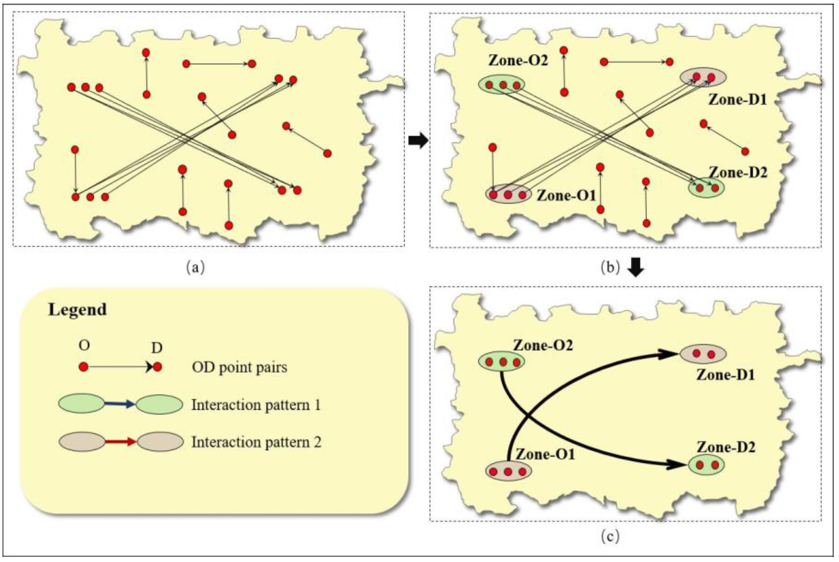
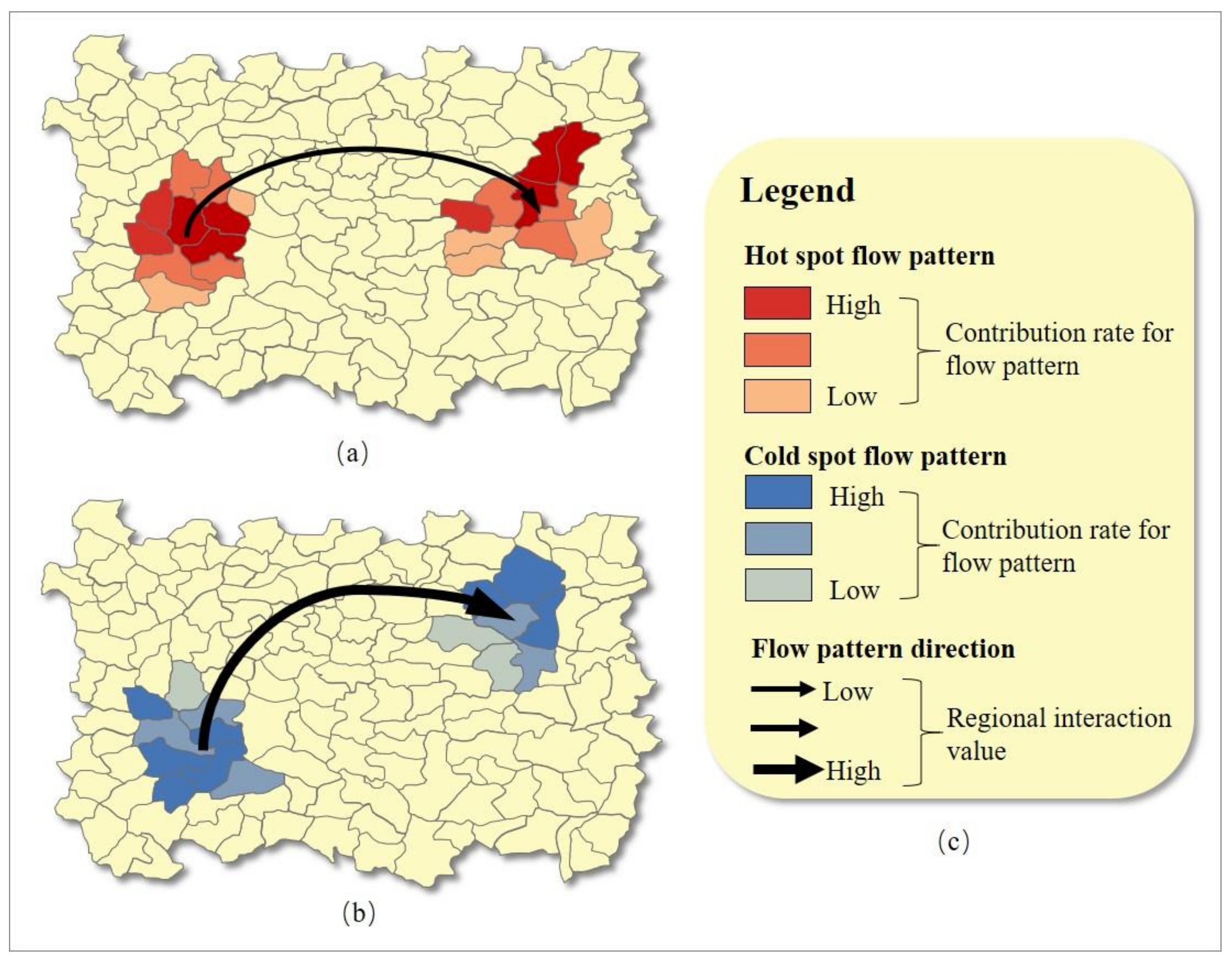
3.2.1. Visualization of a Single RG-Flow-Pattern

In the proposed RG-Flow-Pattern method, analytical results are evaluated and investigated by using different flow pattern variables. These variables enable the assessment of the starting and ending regional groups and the comprehensive assessment of the interaction model. Presenting evaluation variables that match a particular pattern in tabular form is not conducive to spatial pattern analysis and precludes the mapping and further visual analysis of spatial data analysis results. Designing a scientific and reasonable RG-Flow-Pattern visualization method is crucial. Thus, the RG-Flow-Pattern visualization method is designed as shown in Figure 6a,b. Figure 6a,b are two basic examples of RG-Flow-Pattern visualization. The basic meanings and expressions of the two examples are described in detail below.
As we mentioned earlier, a complete RG-Flow-Pattern contains three basic constructs, namely, the starting regional group, the termination regional group, and directional arrows. The size of the interaction value and the contribution rate of each RG-Flow-Pattern to each of the start and termination regional groups and some visual variables, such as color and size, are expressed to visualize the results of each RG-Flow-Pattern. Figure 6a,b show that if one proceeds from the basic definition, the basic requirements of the RG-Flow-Pattern structure are satisfied.
Comparing the two findings reveals remarkable differences in the overall color tone of the regional groups. The regional group shown in Figure 6a has a warm tone, whereas that in Figure 6b has a cool tone. The strength of each RG-Flow-Pattern is expressed by the warmth or coolness of color tones. A warm tone indicates that the RG-Flow-Pattern behaves in a strong interactive pattern, and a cool tone indicates that the RG-Flow-Pattern behaves in a weak interactive pattern. The degree of strength is measured on the basis of the P value obtained through Equation (2). The critical value of strength is divided in accordance with the overall distribution of P values of all models by using natural discontinuity and quantile methods. The P values can be defined by the user. Figure 6a belongs to the strong regional interaction flow pattern, which is further defined as the hotspot flow pattern. Figure 6b belongs to the weak interactive flow pattern, which is further defined as the cold-spot flow pattern. In addition to the collective differences in the coolness and warmth of the tones of regional groups, the inner regions of each RG-Flow-Pattern differ. This difference represents the contribution rate of a single region to the current RG-Flow-Pattern interaction value. Dark colors are associated with the high contribution rate of the region to the RG-Flow-Pattern interaction value and vice versa. Contribution rate is calculated through Equations (4) and (5). The contribution of a single zone in the starting regional group is used to measure the contribution rate of a single region in the termination regional group for each flow pattern. This rule can be applied to hotspot and cold-spot flow patterns. The first two parts of the legend shown in Figure 6c illustrate the specific meanings and corresponding relationships between the expression flow pattern strength and the contribution rate of interaction values in each region to the visualization results.
In addition, to compensate for the inadequacy of the interaction value that can be used to evaluate the strength of the interaction model, the RG-Flow-Pattern also needs to evaluate the value of the overall model interaction value on the basis of the V value. In the visualization, the size of the V value is expressed by the thickness of the arrow, which indicates the current RG-Flow-Pattern interaction value. Comparing Figure 6a,b shows that although the RG-Flow-Pattern in the former shows a strong flow pattern, the interaction value is smaller than that in the latter. The flow pattern direction portion of Figure 6c provides a legend of the interaction value size relationship.
In addition to directional arrows, the complete visualization result of the RG-Flow-Pattern includes starting and ending regional groups, cool- and warm-toned variable groups that represent the strong and weak P values of the interaction pattern, a saturation visual variable that represents the contribution rate V of a single region to the value of the current pattern interaction value, and a visual arrow variable that represents the size of the flow pattern interaction value.

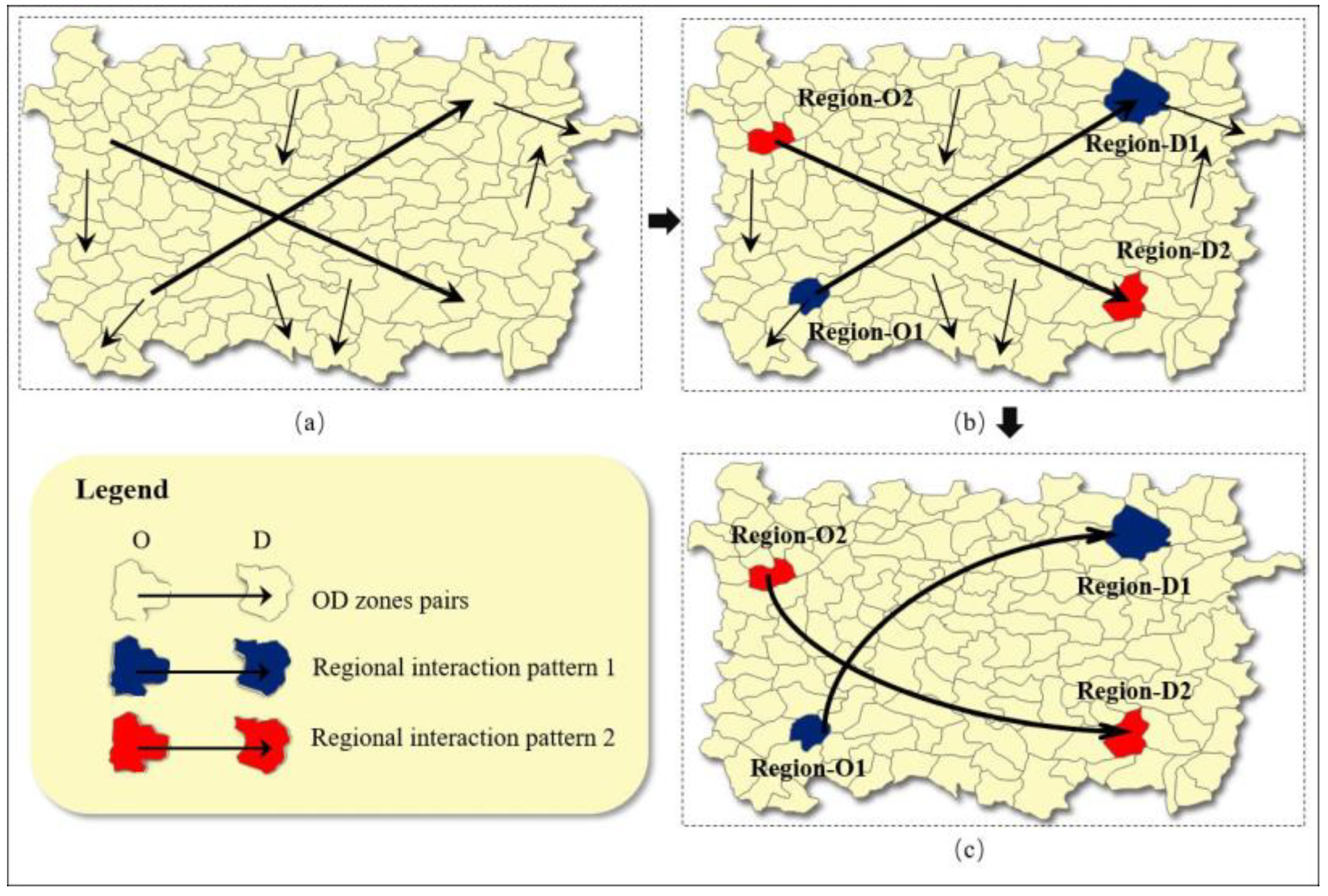
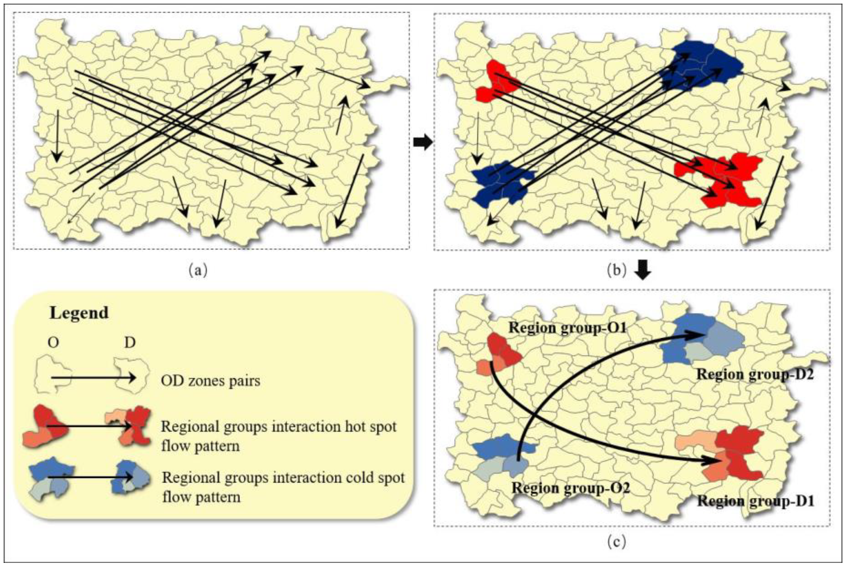
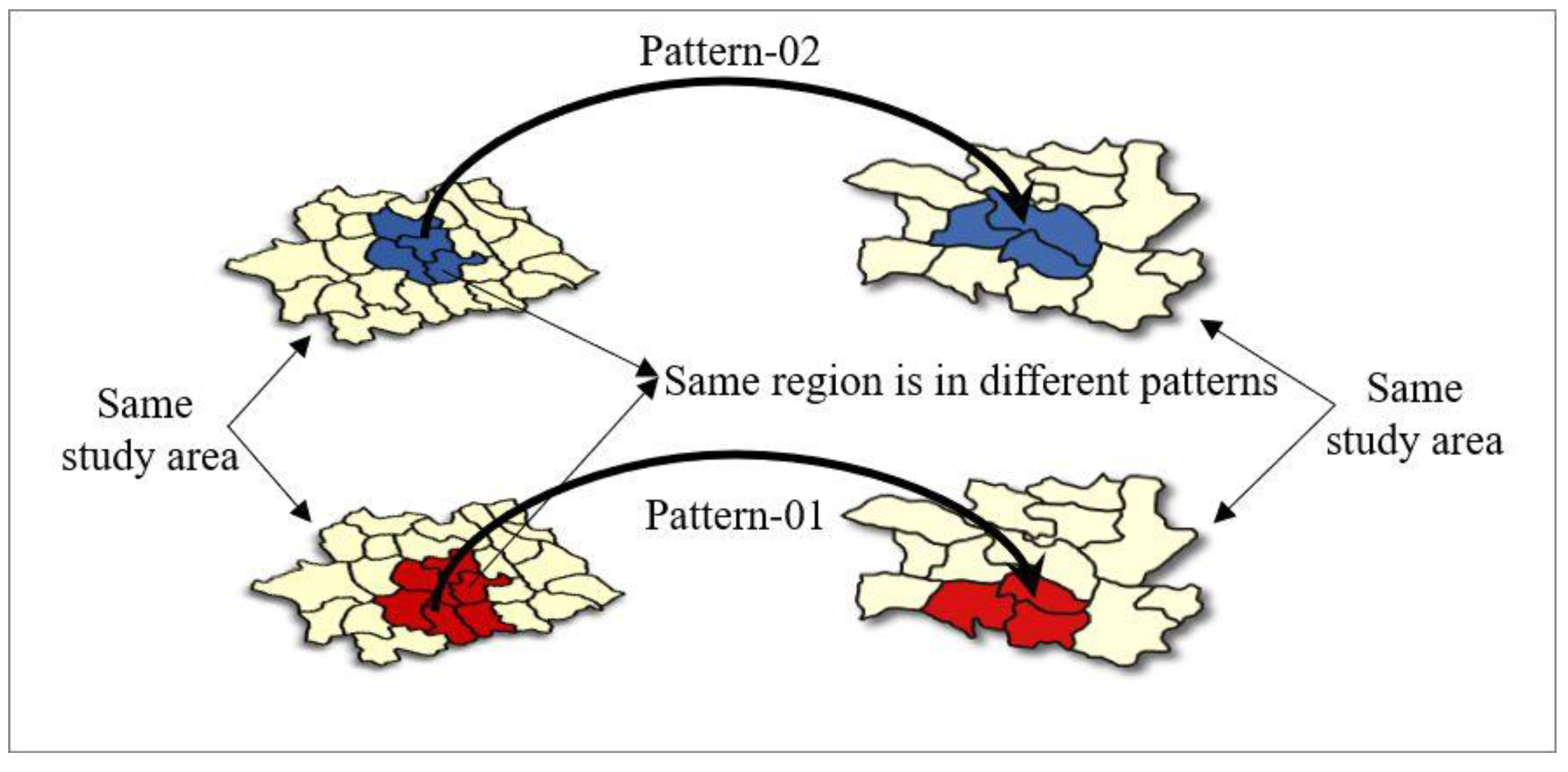
3.2.2. Visualization and Classification of Multiple RG-Flow-Patterns Based on Geo-information Tupu

In the traditional spatial data distribution and visualization patterns, the distribution pattern of the same topic and region can be presented on a map. For example, Local Moran’s I and General G index [39,40], the classical methods for the analysis of the local spatial autocorrelation, facilitate the presentation of model analysis on the same map. However, presenting the regional group interactive hotspot flow pattern on the same map is difficult. Figure 7 shows that although pattern-01 and pattern-02 belong to two different flow patterns in the same region, both patterns have a single repeating unit in the real and termination regional groups. Thus, expressing the two patterns on the same map is difficult for such situations.
The theory and method of geo-information Tupu was originally presented by Chen in the 1990s and can be used to solve this problem [41]. Chen’s geo-information Tupu theory emphasizes the structuring, abstraction, classification, and relevance of the features of geographic laws and uses these principles in a map sequence. The map sequence can be adopted by the geo-information Tupu method because in many cases, presenting multiple RG-Flow-Patterns on the same map is difficult, and the different RG-Flow-Patterns of the same topic can also be divided on the basis of type. The RG-Flow-Pattern map sequence can be arranged in accordance with type, interaction strength, and value size. Only the type division of the RG-Flow-Pattern map is introduced in this work given that interaction strength and values can be directly organized on the basis of P and Z values.
In fact, for RG-Flow-Patterns, type division is also a relatively simple task. In this work, RG-Flow-Patterns are classified into basic and complex types. The basic types mainly include the five types shown in Figure 8.

4. Case Study: National Migration Flow Data of China

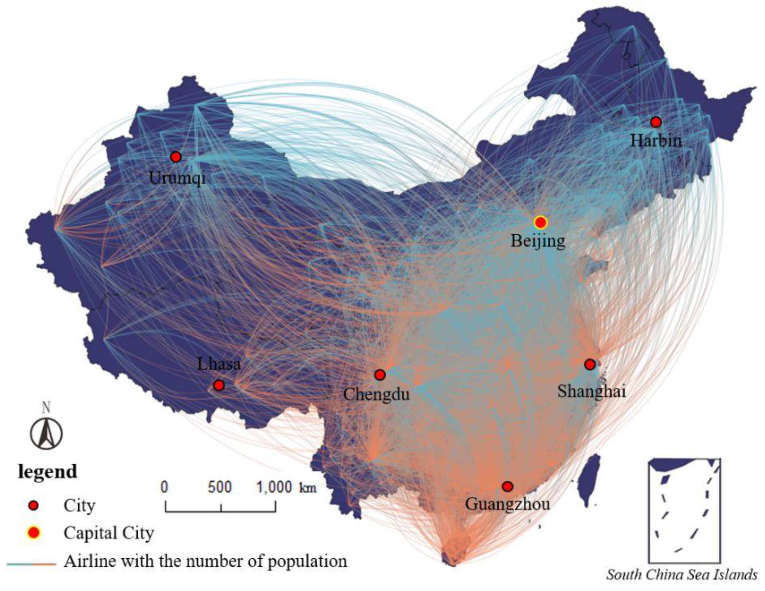
4.1. Study Area and Data Descriptions
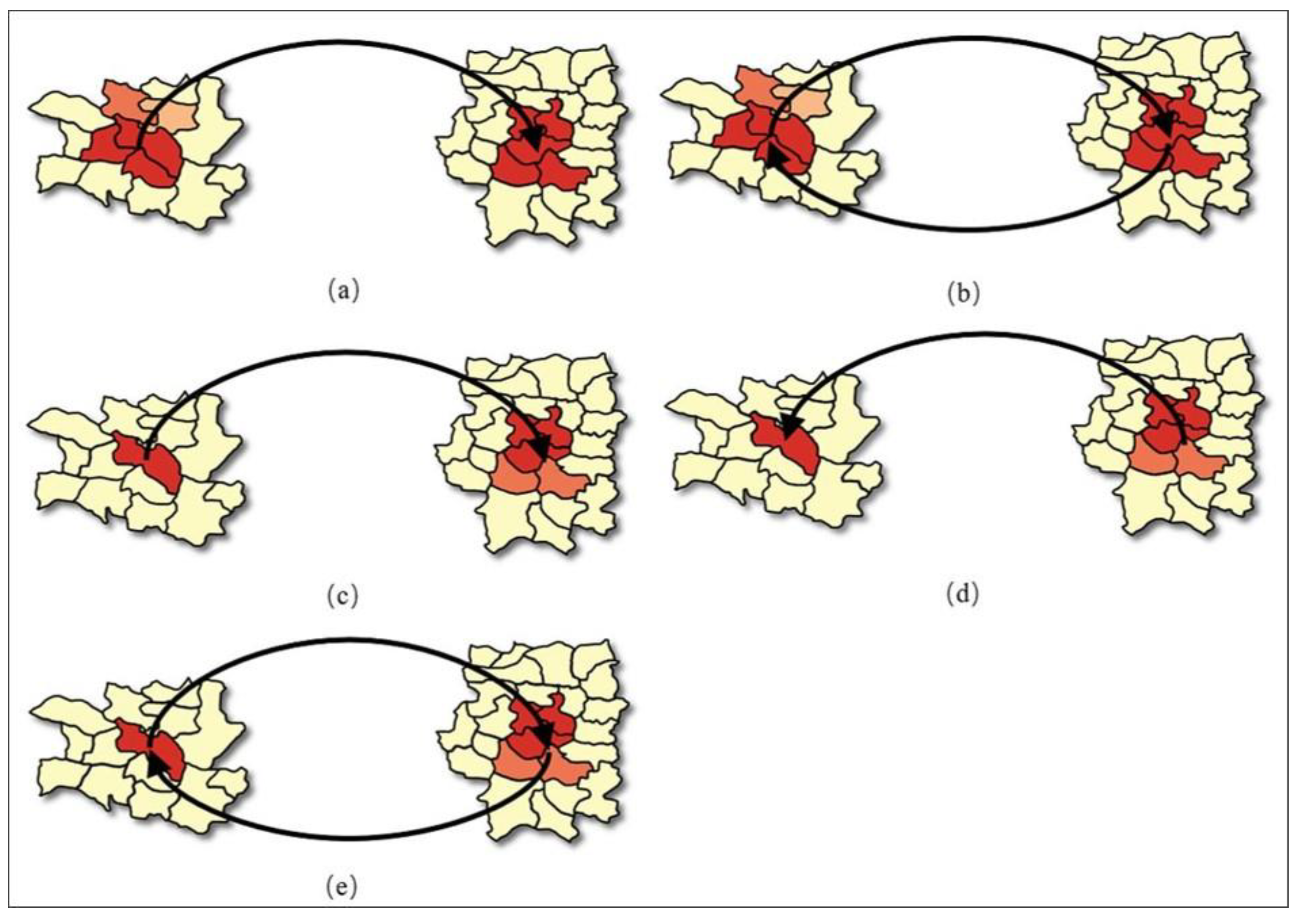
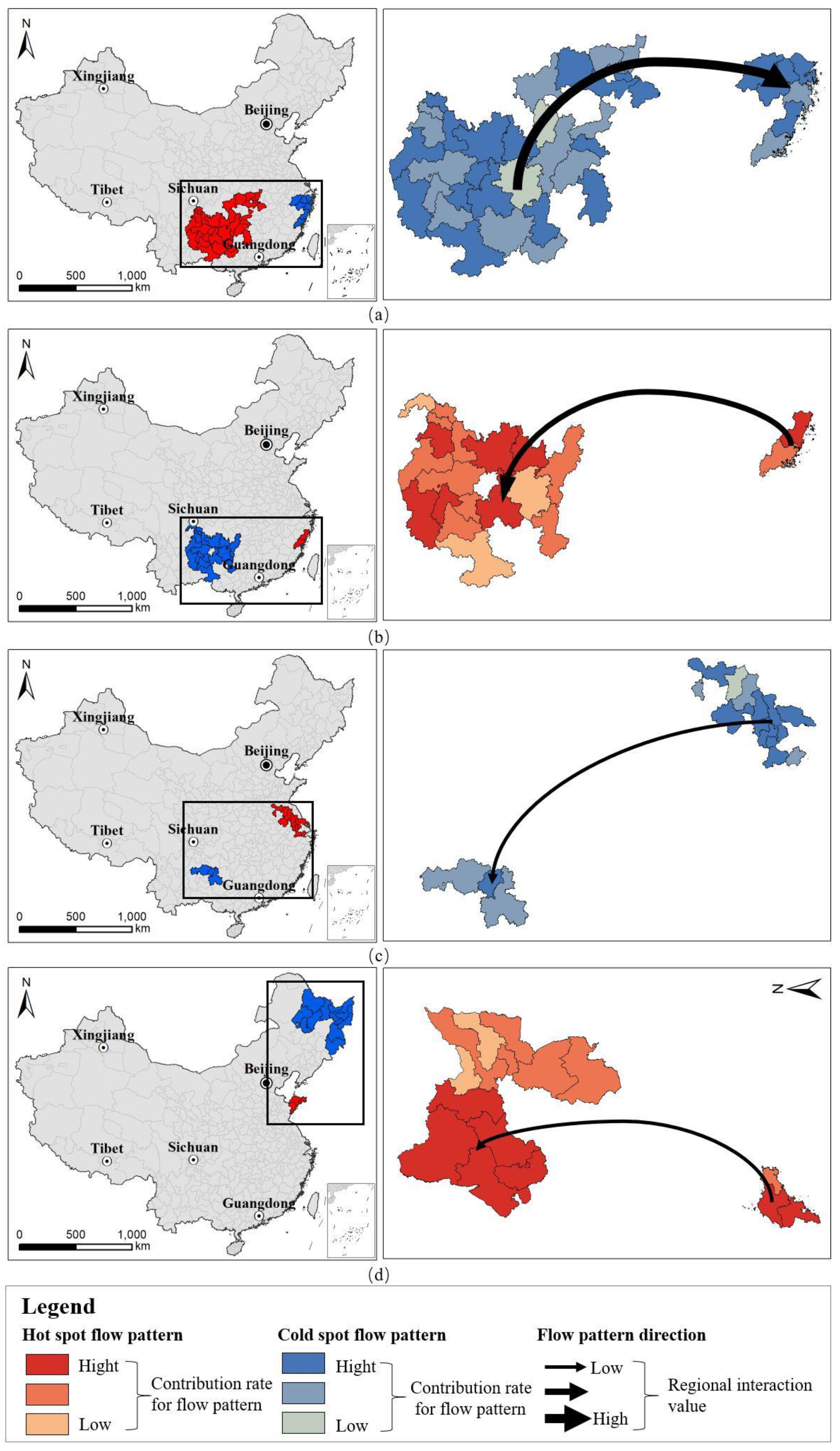
On a daily basis, a large number of people travel from one place to another because of work, leisure travel, or other purposes. Human mobility can reflect many area characteristics, such as urban attractiveness and tourism resources. China has a population of 1.3 billion, and different regions have drastically different economic, political, cultural, and resource characteristics. Massively imbalanced population size and regional disparities further promote population movements [2]. China’s nation-wide cross-regional transportation includes three types of transportation, namely, automobiles, trains, and aircraft. This work uses the migratory flow data of mainland China the main data source with the prefecture-level city as the smallest research unit given its effectiveness in the analysis of flow data across regions. We adopt the RG-Flow-Pattern method for empirical analysis. Figure 9 shows the distribution of population migration routes (by airplane) for the main study area on 1 April 2017. Only the top 10 data inflows and relocations from each prefecture-level city are used in this work.
The demographic data provided by the Tencent location big-data platform are used in this research. Tencent is a major Internet company in China that provides nationwide, location-based, real-time migration big-data services. This platform provides daily migration data for mainland China. Migration types include migration through aircraft, trains, and automobiles. The top 10 regions ranked on the basis of flow data are included, and the degree of the hotspot flow value of inward and outward movement is calculated. Among the three patterns of transportation data, flight data has the longest distance, and the RG-Flow-Pattern method is more effective at analyzing flow data with long distances between the origin and destination areas. Therefore, the population migration data of flights are analyzed in this study. The data used in this study involve 315 cities with approximately 6300 data points and include flow data with original city, destination city, and hot value as the main attributes. The hot value of each directed flow data record is positively correlated with the number of passengers. In our model, the hot value is used as an interaction value in the calculation.
The data used in the experiment consists of two components. A component of the data is the administrative division polygons at the prefecture-level city. These data are mainly used to determine spatial relationships among cities. The other component is the population flow data of flights among different cities. The interaction value between the two cities is measured on the basis of the heat value by mainly using the OD data mining of similar regional group flow patterns. Table 1 shows the main attributes of the two parts of data.

4.2. Result

The RG-Flow-Pattern method proposed in this study was adopted. The prefecture-level city is set as the regional unit, and the modal method of spatial relationship shown in Figure 5c is used. Then, the θ value of P ( R F j ) θ was set to 0.00001. The partial patterns obtained in the analytical results are shown in Figure 10:
Figure 10a shows that RG-Flow-Pattern algorithm identified that some regions in the southwestern part of China (the red part) and the eastern part of the coastal area (the blue part) form the regional group interaction flow model. Figure 10a shows the geographical distribution of the flow pattern on the left, and Figure 10a shows the interaction pattern on the right. The latter shows that the pattern belongs to the cold-spot flow pattern, and the direction of the flow pattern is from the southwest area to the eastern coastal area. The color of a single area represents the contribution of the flow of that area to the entire pattern. The southwest area is used as the starting regional group of the flow pattern, in which the color depth of each area represents the contribution of the sum of the values of the area that flows out to the termination area group to the outflow value (also called the outdegree) of the entire model. The coastal area is the most frequent end-of-flow model, in which the color depth of each area indicates the contribution rate of the inflow value of the area to the inflow value of the entire model. A dark color indicates a high contribution rate.
Figure 10b,d are interactive hotspot flow patterns recognized by the G-Flow-Pattern algorithm. Figure 10c is another set of identified regional group interaction cold-spot flow patterns.

5. Discussion and Conclusions

5.1. Discussion

5.1.1. Principle underlying the Selection of the Regional Adjacency Relationship and Regional Merge Threshold

The adjacent edge-and-corner approach is used to determine the adjacency of an area. In this approach, an area adjoining the target area is considered as adjacent as long as an edge or corner adjacent to the target area exists. Other methods mentioned in Section 3.2.1 can be selected to model the area’s adjacency. However, the use of different regional adjacency relationships may also result in differences in the models based on RG-Flow-Pattern analysis given the effect of regional adjoining relationships on the model. Spatial statistical methods, such as Moran’s I, the Geary index, and geographically-weighted regression, are recommended as a reference for the selection rules of regional spatial relations. Furthermore, when the value of θ in P ( R F j ) θ is different, the resulting flow pattern may also vary. When the value of θ is large, the number of flow patterns to be formed is small. The number of areas in the flow pattern that constitutes the starting and termination area groups also decreases. To solve this problem, the recommended practice is to obtain the P ( R F j ) θ values for all regional flows, and then use the bar histogram to evaluate the distribution of all regional flow P ( R F j ) θ values and select them in accordance with the analytical target. A reasonable threshold is taken as the value of θ . This method can control the number and strength of flow patterns to a certain extent.

5.1.2. Evaluation of Results

A complete flow pattern includes the basic elements of the flow pattern (starting regional group, termination regional group, and interaction arrows), interaction strength, interaction value size, each individual flow pattern, and the rate of contribution of the area’s traffic to the interaction value of the entire flow pattern. Although this design enables each flow pattern to contain sufficient information for self-evaluation, it presents the following disadvantages: First, these assessments are solely for a single-flow model and are insufficient for the assessment of the overall characteristics of all models. For a single-flow pattern, four situations starting from the strength of the pattern and the size of the interaction value are observed: a strong interaction pattern with a large interaction value; a weak interaction pattern with a small interaction value; a strong interaction pattern with a small interaction value; and a weak interaction pattern with a large interaction value. Understanding these four scenarios is useful for the subsequent analysis of the overall characteristics of the model. If the strength and interaction values of each flow pattern can be described by the XY coordinate system, then the four cases can be expressed clearly and transparently by using a four-quadrant diagram.

5.1.3. Shortcomings and Future Improvements

The RG-Flow-Pattern method requires that all flow patterns with certain intensities are recognized from the mass flow data, and a plurality of visual variables are used to express patterns and related evaluation amounts. However, the method exhibits the following deficiencies: First, although this method aims to analyze any type of flow data, such as people, logistics, and traffic flow, it encounters difficulty in finding two cross-regional regional groups with short interaction distance. Thus, this method is suitable for the mining of regional group interaction patterns between regions with long interaction distances. Although one can solve this problem by setting small partitions, more often than not, the interactive areas used for analysis are predefined and show geographic importance and cannot be customized because of their size. In subsequent studies, we will attempt to construct a flow data mining model that is based on this method and that is suitable for short interaction distances. Second, in a complete regional group interaction flow model, a strong self-interactive pattern may exist between a single region of a starting regional group and a single region of an ending regional group. In this case, the RG-Flow-Pattern method cannot recognize their self-interactive pattern. This self-interactive pattern mining method is relatively simple but is mainly challenged by the identification and improvement of the role of the self-interactive pattern in the proposed flow model. Expression is performed visually to facilitate subsequent visual analysis. These are the tasks that require further improvement.

5.2. Conclusions

Geographers have shifted their attention from physical space to flow space because of globalization and the development of the Internet. Methods for spatial analysis have also been extended to the discovery of spatial interaction patterns. Although spatial interaction has always been the focus of the GIS field, spatial interactions and even space-time interactions have attracted the attention of scholars because of the advent of big-data technologies. Numerous researchers mainly focus on point-to-point, area-to-area, or interaction-based research on regional convergence or diffusion but few have considered the interaction patterns that may exist between regional groups with adjoining relationships. In fact, the interaction of most flow data does not only exist between two separate areas but also between a group of areas and another regional group.
We assume that an imbalance in certain resources results in the development of a relationship between one area and another. Furthermore, under the condition of resource imbalances, the surrounding area of one certain region has a similar demand for a certain resource, thereby causing the target area and its surroundings with limited sources (regional groups) to interact with other regional groups with abundant resources. The proposed RG-Flow-Pattern analysis and visualization method can effectively mine the possible interaction patterns between two regional groups under such scenarios. In this analytical method, all regional groups with interaction relationships that satisfy a specific traffic threshold are identified. Moreover, in our proposed method, the strength level of each group of interaction flow patterns, the interaction size of the patterns, and each of the interaction variables and the extent to which the area contributes to the overall model interaction volume can be measured on the basis of the outcome variables.
The first law of geography is the basic principle of the GIS spatial analysis model, that is, the spatial unit has spatial correlation characteristics [42]. In the past, spatially distributed characteristics tend to be considered in analytical models of spatial distributions and relationships. Concomitant with the “interactive” turn of the GIS analysis model and from the perspective of flow space, the spatial flow model or spatial interaction model should also consider spatial correlation. However, the spatial flow model is more complex than spatial distribution and relationship models, and visualizing all patterns on a single map is difficult. In this work, we proposed a method for the analysis of spatial group interaction models based on the relevance of neighboring regional units. Moreover, we used the geo-information Tupu [41] method to express analytical results and address the difficulty of single-diagram visualization. Our analysis and visualization method can be extended to mine data on regional interaction relationships in any other flow data forms. If the target OD data is in point-to-point form, then the OD data based on a certain area unit must be summarized and the RG-Flow-Pattern model must be used for pattern mining. When the OD data itself is based on a certain area unit, then the RG-Flow-Pattern model can be used directly.

Abbreviations

Point-to-pointFrom one point to another point
Area-to-areaFrom one area to another area
Areas-to-areasFrom a group of areas to another group of areas
RG-Flow-PatternRegional Group Flow Patterns

Author Contributions

Conceptualization, H.Z., X.Z. and G.T.; Methodology, X.Z. and H.Z.; Software, H.Z and X.Z.; Formal Analysis, X.Z., H.Z. and X.G.; Data Curation, H.Z. and X.Z.; Writing-Original Draft Preparation, H.Z.; Writing-Review & Editing, X.Z., H.Z., X.G., and L.Z.; Visualization, H.Z. and X.Z.; Supervision, G.T. and G.J.; Project Administration, G.T., G.J. and L.Z.; Funding Acquisition, G.T., G.J. and L.Z.

Funding

This research was funded by [National Natural Science Foundation of China] Grant No. [41671389, 41701185 and 41471371], and by [Jiangsu Natural Science Foundation of Youth] Grant No. [BK20160893].

Acknowledgments

The authors would like to thank the editor and the four anonymous reviewers for their helpful feedback.

Conflicts of Interest

The authors declare no conflict of interest.

References

  1. Marty, P.F. An introduction to digital convergence: Libraries, archives, and museums in the information age. Libr. Quart. 2010, 80, 1–5. [Google Scholar] [CrossRef]
  2. Andris, C.; Liu, X.; Ferreira, J. Challenges for social flows. Comput. Environ. Urban Syst. 2018, 70, 197–207. [Google Scholar] [CrossRef]
  3. Andris, C. Integrating social network data into GISystems. Int. J. Geogr. Inf. Sci. 2016, 30, 2009–2031. [Google Scholar] [CrossRef]
  4. Midler, J.C. Non-euclidean geographic spaces: Mapping functional distances. Geogr. Anal. 2010, 14, 189–203. [Google Scholar] [CrossRef]
  5. Alamri, S.; Taniar, D.; Safar, M.; Al-Khalidi, H. A connectivity index for moving objects in an indoor cellular space. Pers. Ubiquit. Comput. 2014, 18, 287–301. [Google Scholar] [CrossRef]
  6. Wang, J.F.; Li, X.H.; Christakos, G.; Liao, Y.L.; Zhang, T.; Gu, X.; Zheng, X.Y. Geographical detectors-based health risk assessment and its application in the neural tube defects study of the heshun region, china. Int. J. Geogr. Inf. Sci. 2010, 24, 107–127. [Google Scholar] [CrossRef]
  7. Limtanakool, N.; Schwanen, T.; Dijst, M. Developments in the dutch urban system on the basis of flows. Reg. Stud. 2009, 43, 179–196. [Google Scholar] [CrossRef]
  8. McKenzie, G.; Janowicz, K.; Gao, S.; Gong, L. How where is when? On the regional variability and resolution of geosocial temporal signatures for points of interest. Comput. Environ. Urban. 2015, 54, 336–346. [Google Scholar] [CrossRef]
  9. Tao, R.; Thill, J.C. Spatial cluster detection in spatial flow data. Geogr. Anal. 2016, 48, 355–372. [Google Scholar] [CrossRef]
  10. Seto, K.C.; Reenberg, A.; Boone, C.G.; Fragkias, M.; Haase, D.; Langanke, T.; Marcotullio, P.; Munroe, D.K.; Olah, B.; Simon, D. Urban land teleconnections and sustainability. Proc. Natl. Acad. Sci. USA 2012, 109, 7687–7692. [Google Scholar] [CrossRef] [PubMed] [Green Version]
  11. Zhu, X.; Guo, D.S. Mapping large spatial flow data with hierarchical clustering. Trans. GIS 2014, 18, 421–435. [Google Scholar] [CrossRef]
  12. Adams, P.C. A taxonomy for communication geography. Prog. Hum. Geogr. 2011, 35, 37–57. [Google Scholar] [CrossRef]
  13. Mesbah, M.; Currie, G.; Lennon, C.; Northcott, T. Spatial and temporal visualization of transit operations performance data at a network level. J. Transp. Geogr. 2012, 25, 15–26. [Google Scholar] [CrossRef]
  14. Fonte, C.C.; Fontes, D.; Cardoso, A. A web GIS-based platform to harvest georeferenced data from social networks: Examples of data collection regarding disaster events. Int. J. Online Eng. 2018, 14, 165–172. [Google Scholar] [CrossRef]
  15. Hale, M.L.; Ellis, D.; Gamble, R.; Walter, C.; Lin, J. Secuwear: An open source, multi-component hardware/software platform for exploring wearable security. In Proceedings of the IEEE International Conference on Mobile Services, Combra, Portugal, 27 June–2 July 2015. [Google Scholar]
  16. Li, M.; Sun, Y.R.; Fan, H.C. Contextualized relevance evaluation of geographic information for mobile users in location-based social networks. ISPRS Int. J. Geo.-Inf. 2015, 4, 799–814. [Google Scholar] [CrossRef]
  17. Li, J.W.; Ye, Q.Q.; Deng, X.K.; Liu, Y.L.; Liu, Y.F. Spatial-temporal analysis on spring festival travel rush in china based on multisource big data. Sustaina.-Basel. 2016, 8, 1184. [Google Scholar] [CrossRef]
  18. Rosvall, M.; Bergstrom, C.T. Maps of random walks on complex networks reveal community structure. Proc. Natl. Acad. Sci. USA 2008, 105, 1118–1123. [Google Scholar] [CrossRef] [PubMed] [Green Version]
  19. Esquivel, A.V.; Rosvall, M. Compression of flow can reveal overlapping-module organization in networks. Phys. Rev. X 2011, 1, 1668–1678. [Google Scholar]
  20. Zhou, M.; Yue, Y.; Li, Q.Q.; Wang, D.G. Portraying temporal dynamics of urban spatial divisions with mobile phone positioning data: A complex network approach. ISPRS Int. J. Geo.-Inf. 2016, 5, 240. [Google Scholar] [CrossRef]
  21. Kempinska, K.; Longley, P.; Shawe-Taylor, J. Interactional regions in cities: Making sense of flows across networked systems. Int. J. Geogr. Inf. Sci. 2018, 32, 1348–1367. [Google Scholar] [CrossRef]
  22. Kim, K.; Oh, K.; Lee, Y.K.; Kim, S.; Jung, J.Y. An analysis on movement patterns between zones using smart card data in subway networks. Int. J. Geogr. Inf. Sci. 2014, 28, 1781–1801. [Google Scholar] [CrossRef]
  23. Chen, Z.L.; Gong, X.; Xie, Z. An analysis of movement patterns between zones using taxi GPS data. Trans. GIS 2017, 21, 1341–1363. [Google Scholar] [CrossRef]
  24. Liu, L.A.; Hou, A.Y.; Biderman, A.; Ratti, C.; Chen, J. Understanding individual and collective mobility patterns from smart card records: A case study in Shenzhen. Intell. Transp. Syst. 2009, 1–6. [Google Scholar] [CrossRef]
  25. Munizaga, M.A.; Palma, C. Estimation of a disaggregate multimodal public transport origin-destination matrix from passive smartcard data from Santiago, Chile. Transp. Res. C-Emer. 2012, 24, 9–18. [Google Scholar] [CrossRef]
  26. Ghasemzadeh, M.; Fung, B.C.M.; Chen, R.; Awasthi, A. Anonymizing trajectory data for passenger flow analysis. Transp. Res. C-Emer. 2014, 39, 63–79. [Google Scholar] [CrossRef]
  27. Zhang, Y.P.; Martens, K.; Long, Y. Revealing group travel behavior patterns with public transit smart card data. Travel Behav. Soc. 2018, 10, 42–52. [Google Scholar] [CrossRef]
  28. Chu, K.K.A.; Chapleau, R. Enriching archived smart card transaction data for transit demand modeling. Transp. Res. Rec. 2008, 2063, 63–72. [Google Scholar] [CrossRef]
  29. Higuchi, T.; Shimamoto, H.; Uno, N.; Shiomi, Y. A trip-chain based combined mode and route choice network equilibrium model considering common lines problem in transit assignment model. Procedia-Soc. Behav. Sci. 2011, 20, 354–363. [Google Scholar] [CrossRef]
  30. Concas, S.; DeSalvo, J.S. The effect of density and trip-chaining on the interaction between urban form and transit demand. J. Public Transp. 2014, 17, 16–38. [Google Scholar] [CrossRef]
  31. Zhou, L.; Ji, Y.X.; Wang, Y.Z. Analysis of public transit trip chain of commuters based on mobile phone data and GPS data. In Proceedings of the International Conference on Transportation Information Safety, Edmonton, AB, Canada, 8–10 August 2017. [Google Scholar]
  32. Blythe, P.T. Improving public transport ticketing through smart cards. In Proceedings of Institution of Civil Engineers-Municipal Engineer; Thomas, Telford, Ltd.: London, UK, 2004; Volume 157. [Google Scholar]
  33. Pelletier, M.P.; Trepanier, M.; Morency, C. Smart card data use in public transit: A literature review. Transp. Res. C-Emer. 2011, 19, 557–568. [Google Scholar] [CrossRef]
  34. Wang, Y.; Lim, E.P.; Hwang, S.Y. Efficient algorithms for mining maximal valid groups. Vldb. J. 2008, 17, 515–535. [Google Scholar] [CrossRef]
  35. Aung, H.H.; Tan, K.L. Discovery of evolving convoys. Sci. Stat. Database Manag. 2010, 6187, 196–213. [Google Scholar]
  36. Li, Y.X.; Bailey, J.; Kulik, L. Efficient mining of platoon patterns in trajectory databases. Data & Knowl. Eng. 2015, 100, 167–187. [Google Scholar]
  37. Williams, H.J.; Holton, M.D.; Shepard, E.L.C.; Largey, N.; Norman, B.; Ryan, P.G.; Duriez, O.; Scantlebury, M.; Quintana, F.; Magowan, E.A.; et al. Identification of animal movement patterns using tri-axial magnetometry. Mov. Ecol. 2017, 5, 6. [Google Scholar] [CrossRef] [PubMed]
  38. Bunting, R.J.; Chang, O.Y.; Cowen, C.; Hankins, R.; Langston, S.; Warner, A.; Yang, X.X.; Louderback, E.R.; Sen Roy, S. Spatial patterns of larceny and aggravated assault in Miami-Dade County, 2007–2015. Prof. Geogr. 2018, 70, 34–46. [Google Scholar] [CrossRef]
  39. Grieve, J. A regional analysis of contraction rate in written standard American English. Int. J. Corpus Linguis. 2011, 16, 514–546. [Google Scholar] [CrossRef]
  40. Zhang, S.L.; Zhang, K. Comparison between general moran’s index and getis-ord general g of spatial autocorrelation. Acta Sci. Nat. Univ. Sunyatseni 2007, 46, 93–97. [Google Scholar]
  41. Ye, Q.; Tian, G.; Liu, G.; Ye, J.; Yao, X.; Liu, Q.; Lou, W.; Wu, S. Tupu methods of spatial-temporal pattern on land use change. J. Geogr. Sci. 2004, 14, 131–142. [Google Scholar]
  42. Tobler, W.R. A computer movie simulating urban growth in the Detroit region. Econ. Geogr. 1970, 46, 234–240. [Google Scholar] [CrossRef]
Figure 1. Example and analytical methods for point-to-point flow data. (a) Point-to-point flow data, (b) points-to-points flow data, and (c) points-to-points flow patterns.
Ijgi 07 00328 g001
Figure 2. Example and analytical methods for regional flow data. (a) Area-to-area flow data; (b) area-to-area flow data with high interaction values; and (c) area-to-area flow patterns.
Ijgi 07 00328 g002
Figure 3. Flow pattern and visualization of interaction hotspots between regional groups. (a) Area-to-area flow data; (b) area-to-area flow data and area pairs with high interaction values; and (c) similar hotspot flow patterns between regional groups.
Ijgi 07 00328 g003
Figure 4. Overview of the framework for the analysis and visualization of similar flow hotspot patterns between regional groups.
Ijgi 07 00328 g004
Figure 5. Regional adjacency relationships. (a) Vector areas with the target region; (b) adjacent edge relationship; (c) adjacent edge and corner relationship; (d) customized adjacent range relationship; and (e) logical adjacent relationship.
Ijgi 07 00328 g005
Figure 6. Two examples and instrumental definition of single RG-Flow-Pattern visualization. (a) A regional interaction hotspot flow pattern with low interaction value; and (b) a regional interaction cold-spot flow pattern with high interaction value; and (c) legend of FG-Flow-Pattern.
Ijgi 07 00328 g006
Figure 7. Example of one region belonging to different patterns.
Ijgi 07 00328 g007
Figure 8. Basic categories of RG-Flow-Pattern based on geo-information Tupu. (a) Many-to-many regions and single direction RG-Flow-Pattern; (b) many-to-many region and double direction RG-Flow-Pattern; (c) one-to-many single direction RG-Flow-Pattern; (d) many-to-one single direction RG-Flow-Pattern; and (e) one and many double direction RG-Flow-Pattern.
Ijgi 07 00328 g008
Figure 9. Study area and visualization of flow data.
Ijgi 07 00328 g009
Figure 10. Four examples of RG-Flow-Patterns geo-information Tupu obtained under the threshold of 0.00001. (a) A cold-spot RG-Flow-Pattern; (b) a hotspot RG-Flow-Pattern; (c) a cold-spot RG-Flow-Pattern; (d) a hotspot RG-Flow-Pattern.
Ijgi 07 00328 g010
Table 1. Data attributes description.
Data TypeAttributeMeaningAttribute Type
Administrative polygonscity_nameName of each cityString
Population flow data of flightsorigin_city_nameName of origin cityString
destination_city_nameName of destination cityString
hot_valueHot value between citiesDouble

