
A New Endmember Preprocessing Method for the Hyperspectral Unmixing of Imagery Containing Marine Oil Spills


1
Navigation College, Dalian Maritime University, Dalian 116026, China
2
Environmental Information Institute, Dalian Maritime University, Dalian 116026, China
*
Author to whom correspondence should be addressed.
ISPRS Int. J. Geo-Inf. 2017, 6(9), 286; https://doi.org/10.3390/ijgi6090286
Submission received: 12 July 2017
/
Revised: 17 August 2017
/
Accepted: 6 September 2017
/
Published: 8 September 2017
(This article belongs to the Special Issue Oil and Gas Applications of Remote Sensing and UAV Systems)
Abstract
:The current methods that use hyperspectral remote sensing imagery to extract and monitor marine oil spills are quite popular. However, the automatic extraction of endmembers from hyperspectral imagery remains a challenge. This paper proposes a data field-spectral preprocessing (DSPP) algorithm for endmember extraction. The method first derives a set of extreme points from the data field of an image. At the same time, it identifies a set of spectrally pure points in the spectral space. Finally, the preprocessing algorithm fuses the data field with the spectral calculation to generate a new subset of endmember candidates for the following endmember extraction. The processing time is greatly shortened by directly using endmember extraction algorithms. The proposed algorithm provides accurate endmember detection, including the detection of anomalous endmembers. Therefore, it has a greater accuracy, stronger noise resistance, and is less time-consuming. Using both synthetic hyperspectral images and real airborne hyperspectral images, we utilized the proposed preprocessing algorithm in combination with several endmember extraction algorithms to compare the proposed algorithm with the existing endmember extraction preprocessing algorithms. The experimental results show that the proposed method can effectively extract marine oil spill data.
1. Introduction
Oil pollution is one of the most common forms of marine pollution. It is estimated that approximately 706 million gallons of oil are spilled into the ocean each year [1]. Industrial discharges and urban runoff, oil production, and the routine maintenance of ships during operation account for a significant proportion of this spilt oil. The remainder results from seepage, shipping accidents, or atmospheric circulation [2]. Marine oil spills have become one of the most serious ocean pollution problems because they can degrade ocean ecosystems and affect both the environment and the economy [3].
To address oil spill pollution and prevent large environmental and economic costs, a rapid and accurate response is necessary. Hyperspectral remote sensing offers good coverage and the continuity of observations, as well as rich spectral and spatial data. Thus, it is an efficient way to detect and monitor oil spills over a broad area. Moreover, airborne hyperspectral remote sensing is an effective and rapid tool for the remote detection and mapping of oil spills. During the Deepwater Horizon oil spills, hyperspectral remote sensing data were gathered from aerial flights that were undertaken to assess the extent and magnitude of the surface oil [4].
This paper aims to perform precise oil spill extraction over large ocean surface areas. From earlier studies, we know that the oil species typically involved in oil spill accidents (light diesel, heavy diesel, and jet fuel) often have low reflectance values, similar to that of water. Moreover, the reflectance difference between oil and water is not significant in many spectral channels. Traditional multi-band imagery and panchromatic imagery are not able to extract oil spills on the ocean. Therefore, we used hyperspectral imagery, taking advantage of its continuous imaging characteristics to discriminate oil and water on the ocean surface.
Spectral unmixing analysis has been a desirable exploitation goal from the earliest days of hyperspectral remote sensing up to the present [5]. The main techniques include endmember confirmation, dimensionality reduction, endmember identification, and abundance estimation. Spectral unmixing analysis is, therefore, a unique and important element of hyperspectral imagery analysis. It satisfies real needs and offers considerable advantages over other remote sensing data analysis methods in terms of solving these problems.
Here, we mainly discussed the endmember extraction method. Depending on whether pure pixels exist, we divided the endmember extraction algorithms into two categories. One category includes endmember identification algorithms, including the pixel purity index (PPI) [6], N-FINDR [7], orthogonal subspace projection (OSP) [8], and the vertex component analysis (VCA) [9] methods, as well as others. The other category includes endmember generation algorithms, such as minimum volume simplex analysis (MVSA) [10], simplex identification via variable splitting and augmented Lagrangian (SISAL) method [11], the iterative constrained endmember (ICE) method [12], convex cones analysis (CCA) [13], and iterative error analysis (IEA) [14].
However, none of these methods consider spatial adjacency. The endmember extraction algorithms that incorporate spatial information are subsequently described. The automated morphological endmember extraction (AMEE) algorithm defines a morphological eccentricity index to confirm the possibility of an endmember pixel [15]. The spatial–spectral endmember extraction (SSEE) tool works by analysing a scene in parts to increase the spectral contrast of the low contrast endmembers and improve the potential for these endmembers to be selected [16]. Spatial purity endmember extraction (SPEE) first investigates several initial endmember candidates by their intensity and feature levels, then identifies the endmembers using spatial context and spectral similarity refining.
Moreover, several endmember extraction preprocessing models have recently been proposed [17]. The spatial preprocessing (SPP) algorithm estimates a spatially derived scalar factor for each pixel that relates to the spectral similarity of the pixels lying within a certain spatial neighbourhood. This scalar value is then used to weigh the importance of the spectral information associated with each pixel in terms of its spatial context [18]. The region-based spatial preprocessing for endmember extraction (RBSPP) approach first identifies a collection of spectrally pure constituent spectra. It then expresses the measured spectrum of each mixed pixel as a combination of endmembers weighted by abundances that indicate the proportion of each endmember in the pixel [19]. The spatial-spectral preprocessing (SSPP) method first derives a spatial homogeneity index for each pixel in the hyperspectral image. This index is relatively insensitive to the noise present in the data. At the same time, it performs unsupervised clustering to identify a set of clusters in spectral space. Finally, it fuses the spatial and spectral information by selecting a subset of spatially homogeneous and spectrally pure pixels from each cluster. These pixels constitute the new set of candidates for endmember extraction [20]. The spatial–spectral preprocessing module (SSPM) determines the spectral purity score of the pixels located within spatially homogeneous regions. The algorithm is intended to ensure that the candidate endmembers are not spatial border pixels [21]. Based on selecting the pixels that are in both the spatial edges (SEs) and the spectral extremes (SEs) of the hyperspectral image, SE2PP first uses a parameter to define a homogeneous region and then directly extracts the heterogeneous edge points from large areas of the homogeneous region. At the same time, the algorithm extracts the spectral region for endmember extraction [22]. The above methods are all derived directly from the perspective of the spatial information contained in the imagery and ignore the intrinsic relationships within mixed pixels. In addition, most of them are prone to missing anomalous endmembers.
There is a spectral correlation between different bands in hyperspectral images. The traditional endmember extraction methods include VCA, OSP, and IEA, which only use the spectral information of the pixels and ignore the spatial information of the image. However, the existing preprocessing endmember extraction models [18,19,20,21,22] are intended to consider the continuity of the image space and use the specific parameters of the image to compute the image space over a wide range. There is no doubt that a large computation area leads to a large number of calculations and is time-consuming. Moreover, previous preprocessing models did not fundamentally consider the intrinsic relationships of the pixel formations to extract the endmember candidates.
This paper proposes a novel endmember extraction preprocessing method called the data field-spectral preprocessing (DSPP) algorithm. The method combines data field information (reflecting the intrinsic relationships within pixels) and spectral information to identify candidate endmembers. In addition, endmember extraction methods, such as VCA, OSP, MVSA, and SISAL, are applied to identify the exact endmembers. We apply the fully constrained least squares (FCLS) method based on the linear spectral mixing model to carry out the abundance estimation. Moreover, to assess the performance of the proposed algorithm, we compare it with the SPP, RBSPP, and SSPP preprocessing methods. The flowchart of the DSPP algorithm is shown in Figure 1.
2. Methodology
2.1. Data Field Index Calculation
The feature space is a basic concept in hyperspectral remote sensing studies. Pixels with similar spatial positions are more likely to belong to the same kind of objects than pixels that are far away from each other. In the feature space, the distance between similar pixels is closer and more likely to converge. Mixed pixels are more likely to be located on the boundary between different kinds of objects. However, anomalous endmembers are prone to be located in the sparsest areas in the feature space. A large homogeneous area in an image space has the cluster characteristics of the feature space, while an anomalous endmember appears as an isolated point. Therefore, the traditional preprocessing methods cannot adequately extract abnormal endmembers in large homogeneous areas.
According to the characteristics of physical fields, the structural characteristics of a hyperspectral image in feature space can be described by the data field theory. The data in the feature space are regarded as data particles, which can radiate energy; thus, the entire feature space is projected to the data field space, and each point in the space has a corresponding potential value. Using the field theory from physics as a reference, we introduce the intrinsic interactions of material particles and the corresponding field description to describe an abstract image datum space.
There exist some particles or nuclei of a given mass with a field around them in the space, in which any given object is subject to the force exerted by the other objects. Thereby a data field is determined over the entire space. For static data that do not depend on time, the data field can be considered stable and active. Therefore, given all the intensity vectors or the potential scalars, we can describe the spatial distribution.
From a point within the data field, the pixels are no longer isolated data points. Instead, they represent many particles capable of radiation. A given point radiates energy from itself to the entire area covered by the image. The energy intensity decreases with increasing distance. Any pixel receives energy from the surrounding points; meanwhile, it radiates energy to other points.
The potential energy function is calculated in formula (1) [23]:
where m ≥ 0 denotes the grey value of a pixel; k ∈ N denotes the distance index; and k, which is set to two in this study, represents the Euclidean distance. σ is the impact factor, which is a constant of the data field and describes the potential influence of the pixels on one another. When this factor is small, there is little influence between the pixels, reflecting limited clustering. In such cases, the lines of equal potential also describe independent pixel-centric regions of energy. With increases in the impact factor, increasing interactions between individual data pixels occur, and the line features are closer together. The effects of the impact factor on the endmember extraction tests will be evaluated in the experiments described in Section 3.
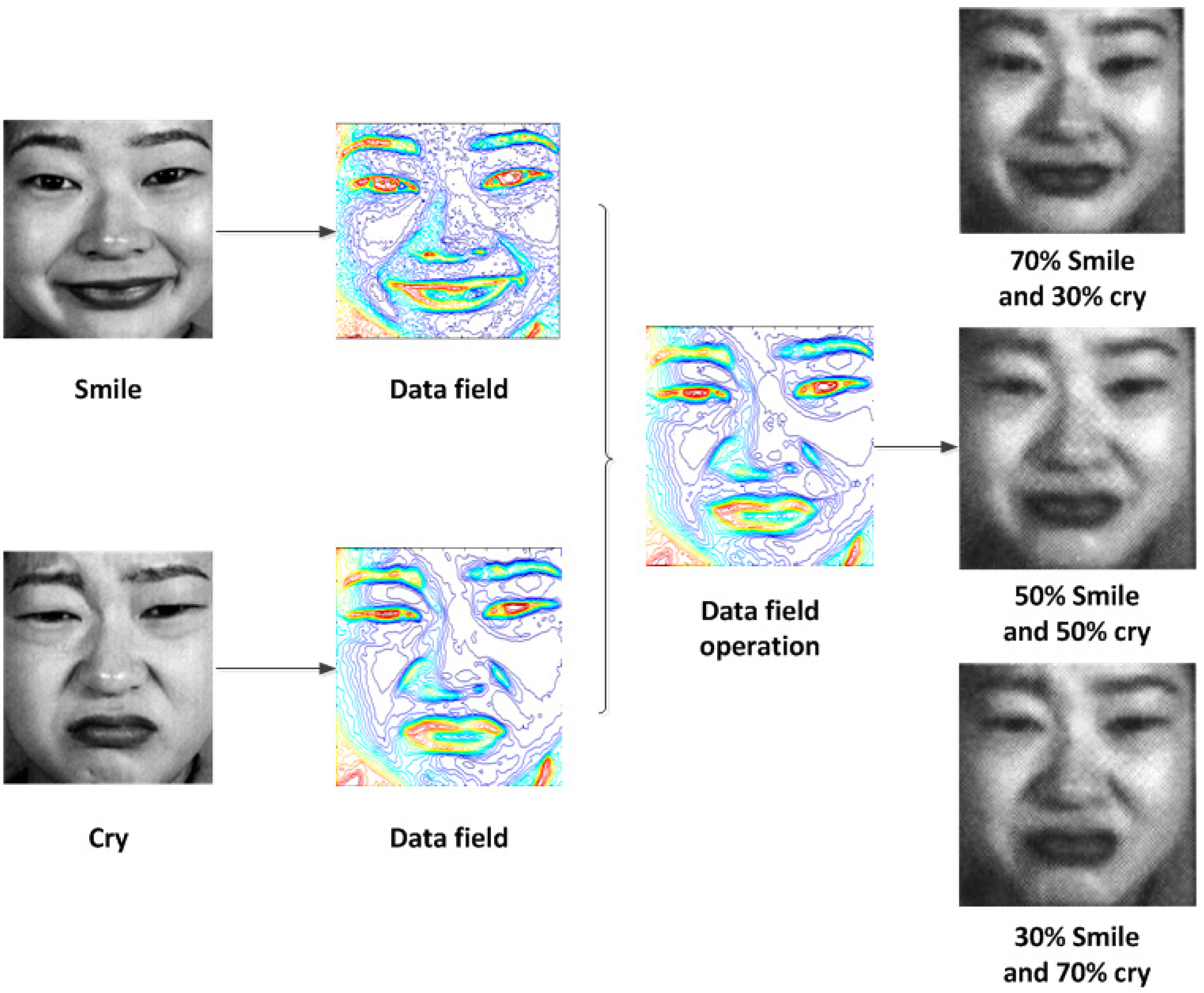
The data field model can effectively and conveniently reflect the distribution of the important feature points (such as the maxima and minima in the data field space) of the original image in different characteristic spaces. Using the field operation of the data field, the original image can be easily transformed through the extraction of feature points. Take a face for example, which can easily demonstrate the function of the data field model, as shown in Figure 2.
Different spatial and spectral characteristics in the local region result in different spatial distributions and different data fields associated with each pixel vector in the image space. We used the potential energy as the feature to extract from the characteristics of the data field, thus achieving the purpose of the endmember extraction preprocessing.
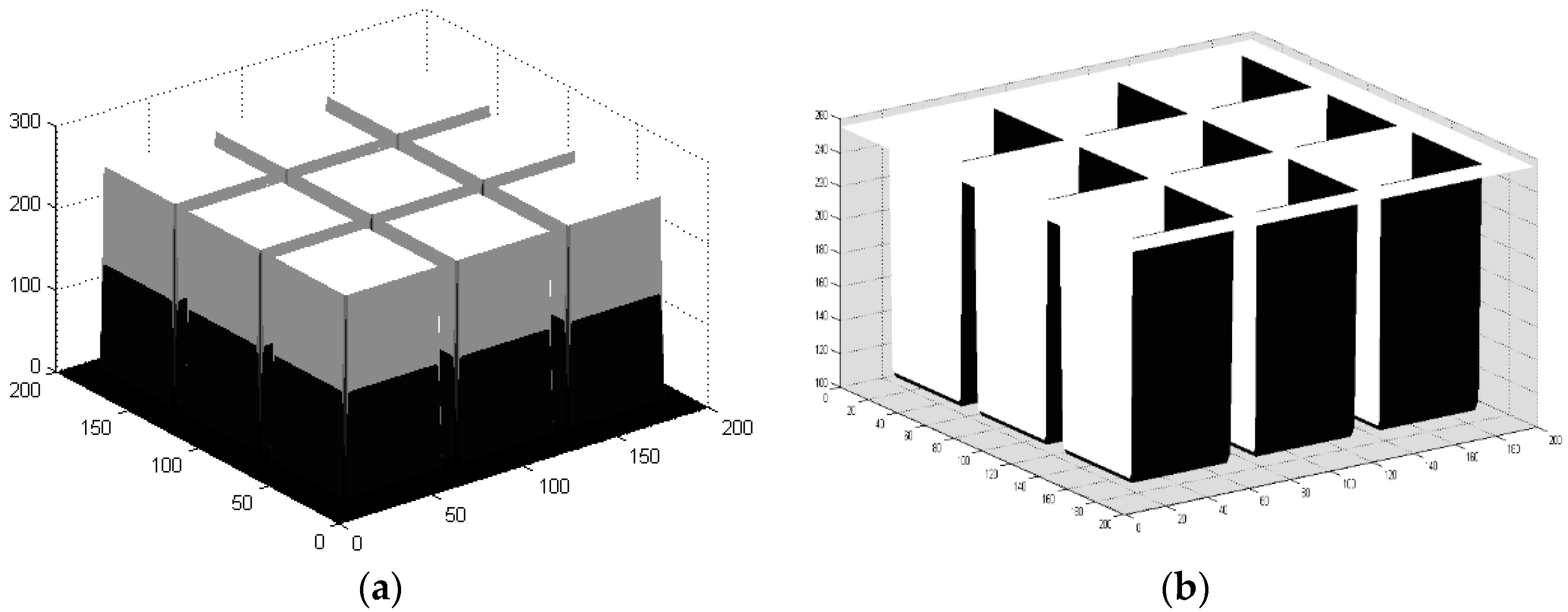
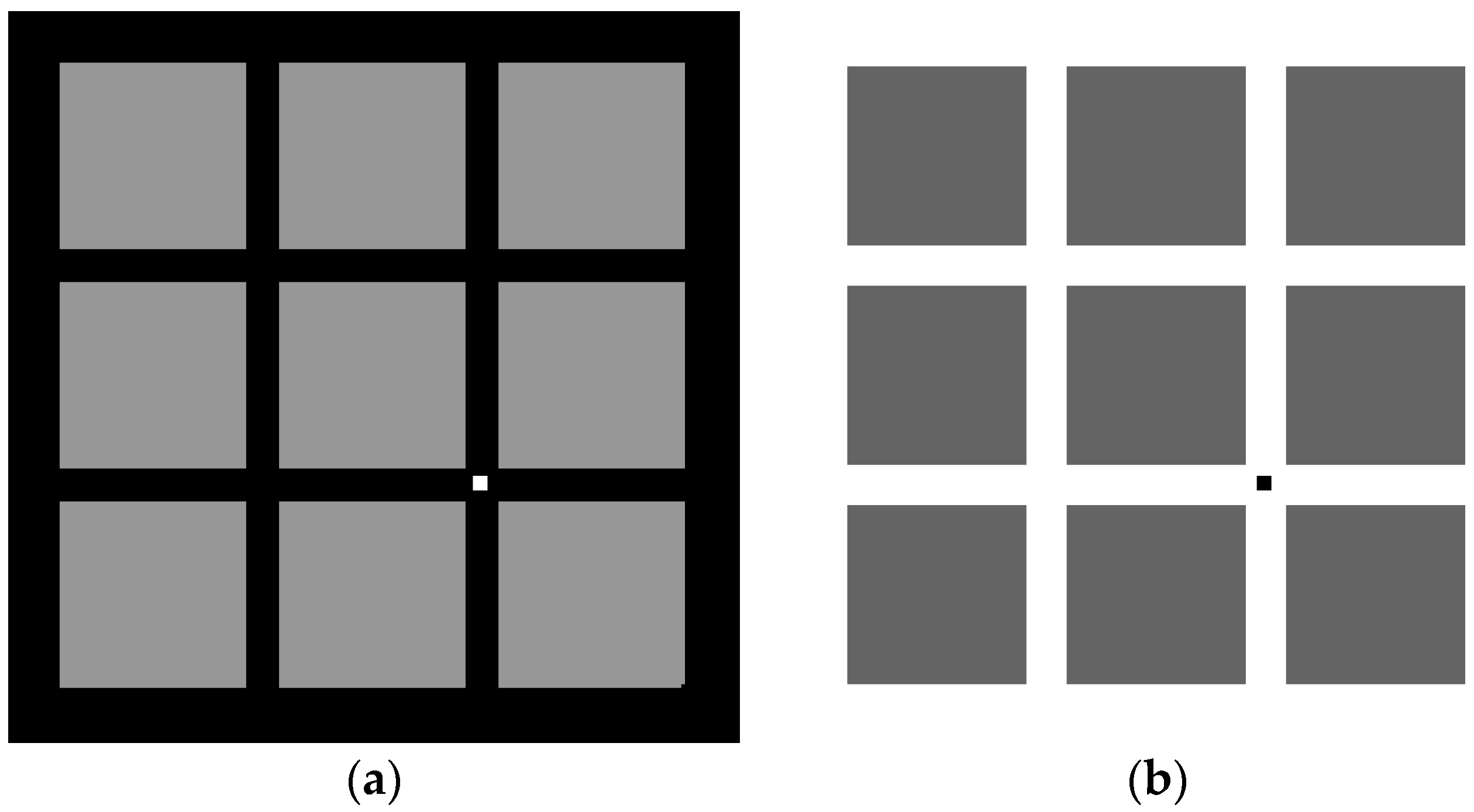
To more deeply explore the characteristics of an image data field, this paper studied the data field properties of central pixels and their neighbouring pixels in an image. We simulated a grid with a background value of = 0 and a foreground value of = 150, and another grid with a background value of = 255 and a foreground value of = 100, as shown in Figure 3. In addition, we also calculated the corresponding image data fields, as shown in Figure 4.
When the centre pixel and the neighbouring pixels of the homogeneous region are relatively high values, they are called the high grey value areas (the nine patches in Figure 3a). Conversely, the homogeneous regions containing low-value pixels are called the low grey value areas (the nine patches in Figure 3b). The data field calculated from the above figure shows that the average potential energy of the high grey areas is also high, so there exists a maximum in the local data field space. In contrast, the potential value of the nine patches is significantly lower than that of the edge region with a higher background value. In addition, both high-value areas and low-value areas are defined as homogeneous regions [24,25]. The normal endmember in the image space we are examining may exist in the geometric centre of a homogeneous region, corresponding to the potential extreme values of the data field space. Therefore, using the data field theory to locate the endmembers corresponds to locating the maximal or minimal points in the data field where the “potential cores” of the homogeneous area are located. The normal candidate endmembers are always located in the “potential cores” of the data field.
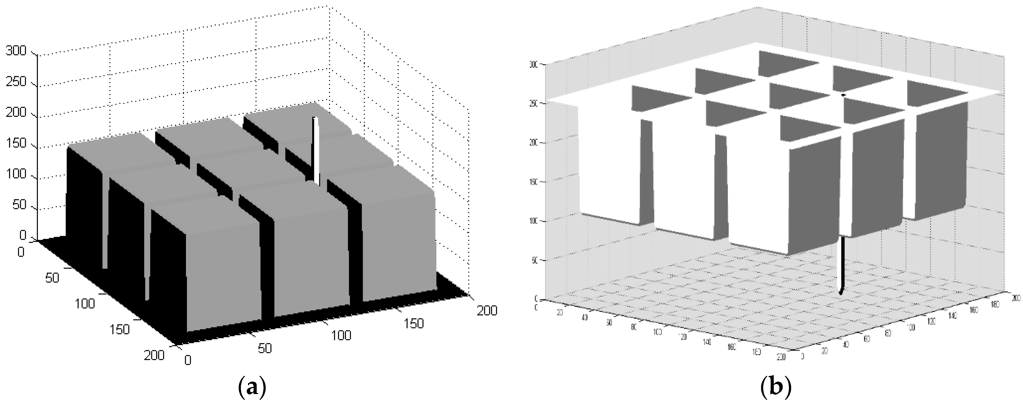
To explore the performance of the anomalous endmember extraction using the data field theory, anomalous pixels were added to the above simulated images. The corresponding data fields were then calculated, as shown in Figure 5 and Figure 6.
The accuracy of the anomalous endmember extraction directly affects the accuracy of the spectral unmixing. It is shown in the above figures that when an anomalous pixel is added to a corner of a simulated image, the anomalous pixel will form an obvious extreme in a neighbouring range of the local data field. On the other hand, the endmember of the homogeneous region will also generate many extreme points in the data field space. Therefore, to extract the extreme in two places, that is, to extract the local potential cores of the image, we can extract the candidate endmembers, including the anomalous endmembers and the homogeneous endmembers. This procedure lays a theoretical foundation for extracting candidate endmembers using data field theory.
In this step, in the process of the data field index calculation, with the help of principal component analysis (PCA) [26], we used the first three principal components of the hyperspectral image and the impact factor σ as the inputs and obtained a set of data field values derived from the input image as the outputs.
2.2. Spectral Clustering
In parallel with the first step, we first determined the endmember number e using the HySime algorithm [27]. In addition, we then applied the unsupervised spectral-based ISODATA algorithm to the original spectral data, where the minimum and the maximum class numbers were all set to e [20].
This step is useful for the next “spectral purity index calculation” process. In this step, during the process of spectral clustering, we inputted the hyperspectral image and the cluster class number and obtained the classified segmentation of the image.
2.3. Spectral Purity Index Calculation
We calculated a spectral purity index similar to the well-known pixel purity index algorithm to identify the most spectrally pure pixels in each cluster (we set the percentage for ranking pure pixels to β). First, a principal component analysis was applied to the entire image. Taking the first components as the direction for example, we computed the maximum and minimum projection values. The pixels with maximum and minimum projection values were assigned weights of 1. We also apply a threshold value; weights that were lower than the threshold were assigned values of 0. The spectral purity index for a given pixel is the sum of all the weights for that pixel over all e principal components.
In this step, we inputted the clustering map from step 2, the percentage of ranking spectrally pure pixels per cluster β, and a weight threshold value δ, and obtained a series of pixels with the greatest spectral purity.
2.4. Fusion of Data Field and Spectral Information
This step takes the data field pixels calculated in step 1 and the spectrally purest pixels identified in step 3 as the inputs. The two index results were calculated by means of a dot product computation, carried out point by point.
Finally, it returned a subset of pixels from the original hyperspectral image, which were preprocessed to subsequently extract the endmembers.
Moreover, in addition to using the DSPP endmember preprocessing algorithms for endmember candidate extraction, we also used OSP, VCA, MVSA, and SISAL to extract the exact endmembers. The reasons why we selected these extraction algorithms are as follows: (1) They are fully automated; (2) They require no additional input parameters other than the endmember number e; (3) The four algorithms can be divided into two groups. OSP and VCA are based on the pure signature assumption, whereas MVSA and SISAL are considered minimum volume methods. Therefore, the latter two algorithms do not assume that the endmembers exist in the image. At last, we applied a fully constrained linear model [28] to complete the hyperspectral unmixing. The result of this process is a set of e endmembers and their corresponding abundance estimation maps.
3. Experimental Results
3.1. Synthetic Data
3.1.1. DSPP Procedure
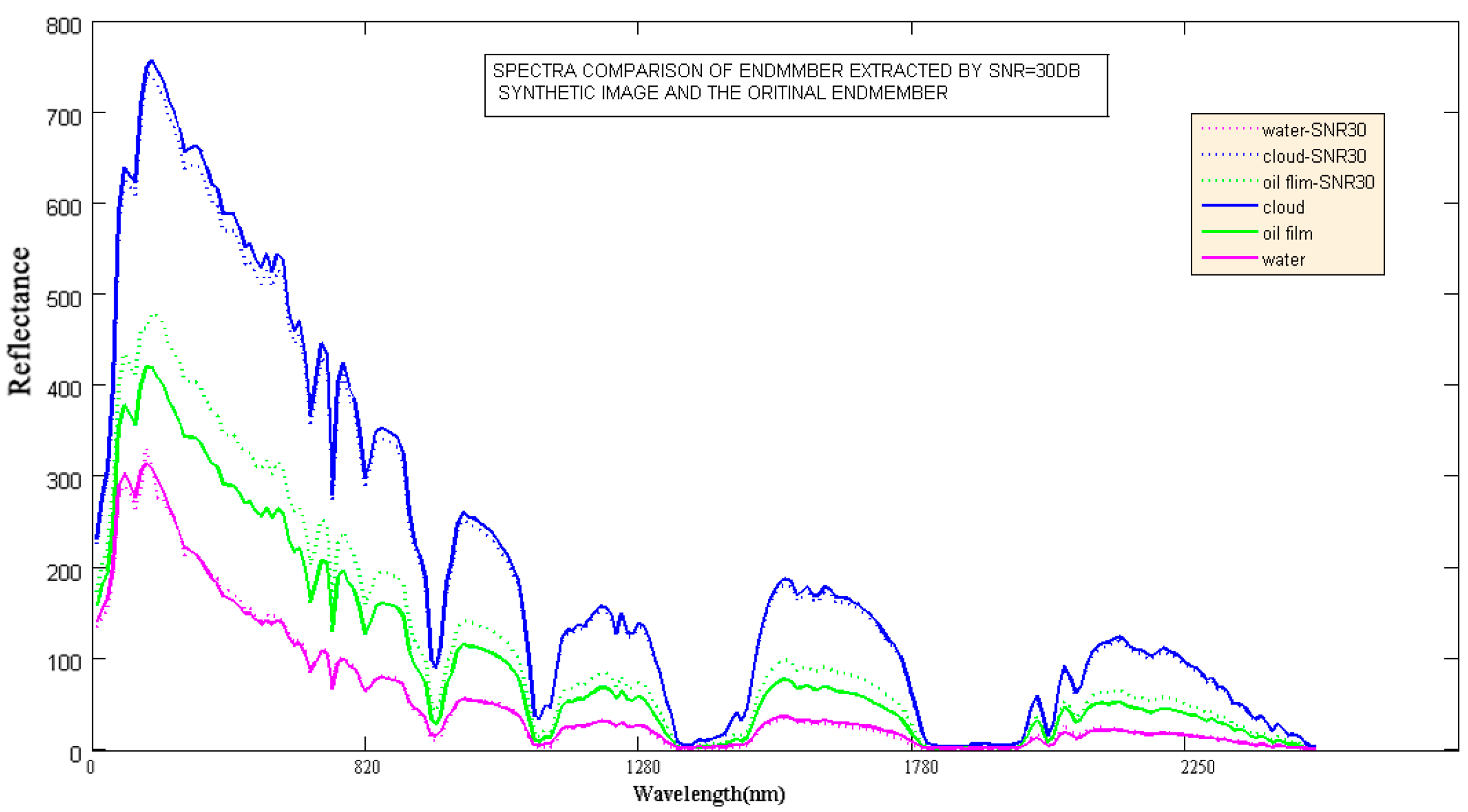
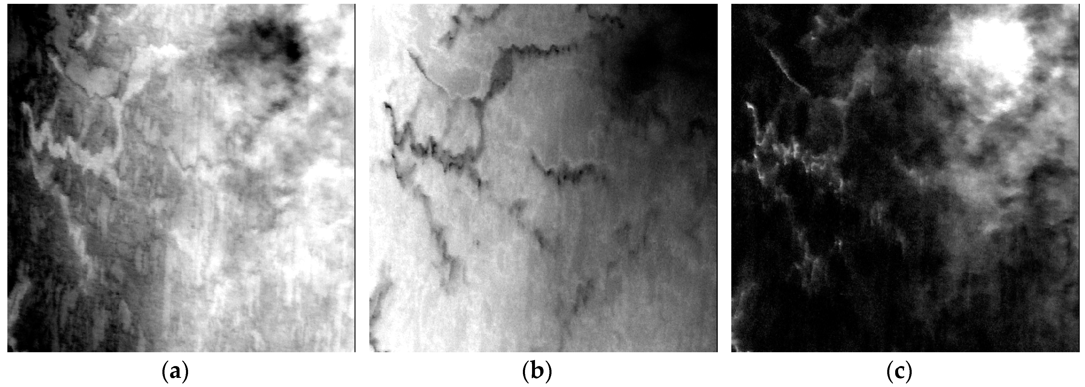
In this paper, we first use synthetic hyperspectral scenes to complement the real images mainly because the details of the simulations are predetermined and controllable. The spectra and abundance of each endmember are known in advance. Therefore, the performance of the algorithm can be validated in a controlled manner. The endmember spectra, which have a total of 224 bands that we chose, are often found in marine oil spill imagery, which includes clouds, oil, and water. Figure 7 shows the endmember spectra, from which we can see that the spectral shapes of these three typical features on the ocean surface are almost the same. The largest difference is found in the absolute value of the spectral differences. In this paper, to promote correspondence with the hyperspectral reflectance values seen in real data, we expanded the endmember reflectance of the synthetic data 10,000 times, from 0 to 10,000. Using the hyperspectral imagery synthesis tools [29], we chose the “Legendre” method to simulate the abundances within the range of 0.1–0.8. The fractional abundances in each pixel of the scene were positive and added up to one, ensuring that all pixel instances in the synthetic fractal image strictly adhered to a fully constrained linear mixture model. In addition, we inputted the ready endmembers. Thus, a database of five 128 × 128-pixel synthetic hyperspectral scenes was created. Figure 8 shows the five synthetic hyperspectral scenes displayed in band 10, band 120, and band 210 (similarly hereinafter).
Next, we computed the potential energy value of the data field of each input image, following formula (1). Each pixel has a potential value, as in geological digital elevation models. We connected the same values within an interval using ‘equipotential lines’. To explore how the different impact factors affected the model, we set the impact factor σ to 0.5, 2, and 5 in succession, as shown in Figure 9.
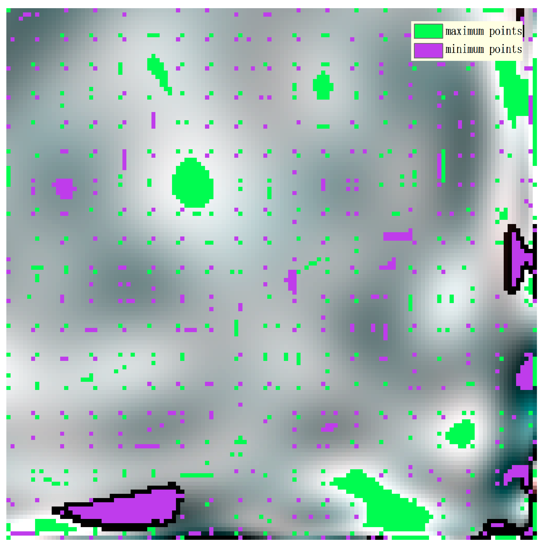
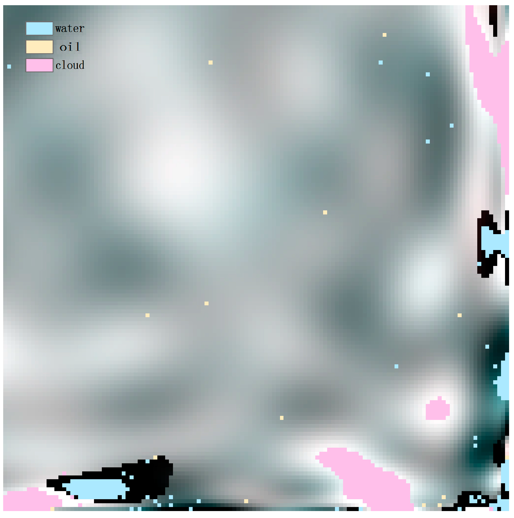
We found that the exact impact factor value does not play an essential role in the synthesis of small images (obviously different areas were drawn in the rectangular frames in Figure 9). The smaller the impact factor, the rougher the potential function curve and the lower the potential energy of the entire data field. Conversely, a greater impact factor means a smoother curve and a higher overall potential energy. However, in this step, we only required a maximum or a minimum in a certain neighbourhood. Through the experiments, we found that the impact factor had little influence on the extraction of the potential cores. Therefore, in the following, we take the impact factor σ to be 2 as an example to complete the experiment. The potential cores were calculated as follows. According to previous image data field theoretical analyses of potential energy, the candidate endmembers always exist as the potential cores within an image. Within a rectangular window neighbourhood with a radius = 5, we obtained maxima equal to the potential peak values, and the minima were the minimum potential values. The peaks and minima represent the sum of the candidate endmembers in this step, as shown in Figure 10. On the other hand, after the unsupervised clustering procedure was conducted with ISODATA for the same synthetic image, the candidate endmembers were calculated using the spectral purity index model (β was set to 30 and δ was set to 1.0), as shown in Figure 11.
The intersection sets of the data field endmember candidates and the spectral purity endmember candidates make up all endmember candidates for the next endmember extraction. Thus, the DSPP preprocessing procedure is complete, and the endmember candidates have been detected.
In the following section, the different endmember extraction algorithms, such as VCA, OSP, MVSA, and SISAL, are applied to the endmember candidates after the procedure described above. We also compare the performance of the proposed DSPP method to that of the other preprocessing procedures in combination with several endmember extraction algorithms. The SPP, RBSPP, and SSPP preprocessing procedure are compared qualitatively and quantitatively.
3.1.2. DSPP Performance Analysis
We compared the performance of the proposed DSPP algorithm with those of the existing SPP, RBSPP, and SSPP algorithms. Together with the VCA, OSP, MVSA, and SISAL endmember extraction algorithms, we obtained the endmember spectra. With the help of the FCLS model, their corresponding abundance maps were estimated. Take the abundance map using DSPP+VCA for example, as shown in Figure 12.
We then calculated the respective reconstructed images for the five original synthetic images. We empirically selected suitable parameter values for each algorithm so that they provided good results in most cases. We set the window size value of SPP to 5. For the SSPP algorithm, the percentage of pixels using the spatially homogeneous index was set to 50, and that of the spectral purity index was set to 30, and the parameter that denotes the spatial context of the given pixel was set to 1.5. Taking one of the synthetic images as an example, the reconstructed images using the above endmember preprocessing algorithms combined with VCA combination are shown in Figure 13.
As is shown in Figure 13, we qualitatively compared the reconstructed images with the original image in Figure 8. We drew the provisional conclusion that the reconstruction using DSPP+VCA is the closest to the original image. In addition, it is clear that the reconstructed images obtained using RBSPP+VCA and SSPP+VCA have many unsmoothed speckles. The results of SPP+VCA are better in this respect, but the spectral value was not similar to that of the original image.
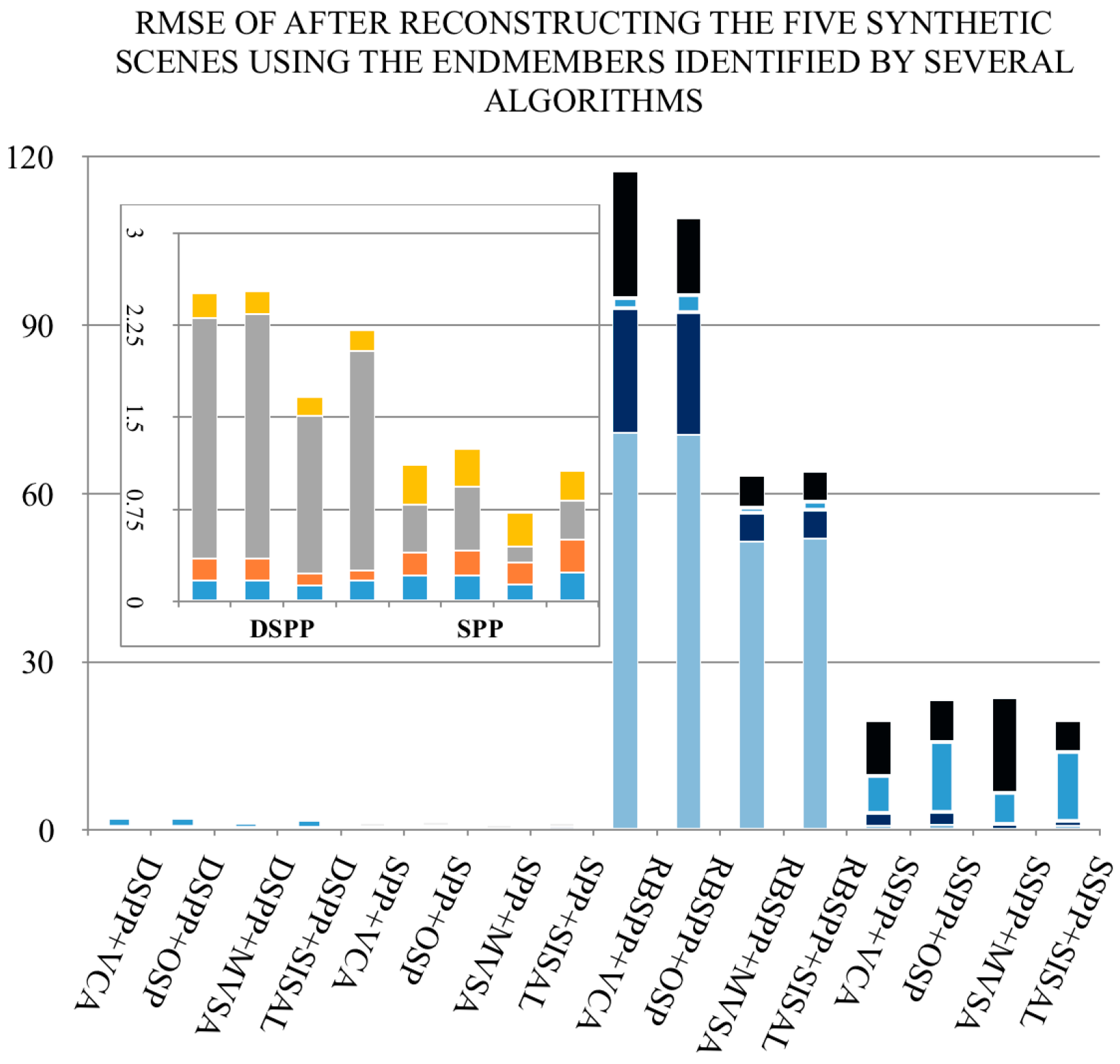
In this paper, we used the root mean square error (RMSE) to compare the original and the reconstructed hyperspectral images. The reconstructed images were generated using the endmembers obtained by the different algorithms and their corresponding abundances, which were estimated by the FCLS model. The RMSE values of the five reconstructed images using several endmember extraction algorithm combinations are shown in Figure 14.
Overall, the performance of SPP is the best. The proposed DSPP is also reasonably good. The RBSPP and SSPP rely primarily on map-based unsupervised classification to ensure spatial homogeneity, so they may have difficulties in extracting the anomalous endmembers. Moreover, in terms of our purpose of discriminating water and oil, which have similar spectra, we found that the MVSA and SISAL algorithms, which do not assume a pure signature, performed better than both VCA and OSP.
To validate the robustness of the proposed DSPP algorithm to noise, Gaussian white noise with a zero mean was added to the different SNRs (30 dB, 70 dB, and 110 dB), following the procedure described in [8]. The SNR is defined here as 50% reflectance divided by the standard deviation of the noise. The SNR = 30 dB synthetic image is shown in Figure 15, and the endmembers extracted using DSPP+VCA with SNR = 30 dB are shown in Figure 16.
In this section, we mainly used three metrics to verify the validation of the proposed preprocessing algorithm. One of these metrics is a spectral similarity measurement (SSM). Under different SNR conditions, we used SSM to assess the similarity among the spectra of the extracted endmembers using several algorithms and the spectra of the original endmembers. The Euclidean distance mainly describes the spectral radiance of the spectral vector difference for hyperspectral image gain sensitivity. On the other hand, while the spectral angle measurement is spectral vector-oriented and therefore represents the shape of the spectrum to some extent, it is insensitive to the gain of hyperspectral images. The above analysis shows that using the Euclidean distance or the spectral angles alone does not accurately reflect the similarity between the spectral vectors. Therefore, we used a combination of spectral angles and Euclidean distances to improve the accuracy of the endmember spectral vector similarity. The spectral similarity measurement was calculated as shown in formula (2).
The average SSM values of the five synthetic images are shown in Table 1. The smaller the SSM value, the more similar the extracted endmember spectra are to the original spectral and the better the performance.
From Table 1, similar to the above no-noise synthetic results, we can also say that the proposed DSPP algorithm yielded a better performance than the other preprocessing algorithms when oil, water, and clouds were the endmembers, which is consistent with our purpose of identifying marine oil spills. The SSM was always small, and it achieved a minimum value at low noise values. In addition, the performance of the SPP algorithm was also quite good, and the spectral similarity was always small. With increasing noise, the algorithm yielded stable results. Based on VCA, OSP, MVSA, and SISAL, we found that VCA performed much better in terms of its robustness to noise; the VCA endmember extraction algorithm that we applied included a module that estimates noise.
The next metric we used was the RMSE (discussed above), which was calculated between the original synthetic images and the FCLS-reconstructed images generated using the endmembers by the different combined algorithms. The calculated RMSE values are shown in Table 2.
The RMSE results were similar to the spectral similarity measurements. We concluded that our proposed DSPP and the existing SPP methods were consistently better. In addition, the results from RBSPP and SSPP were not satisfactory in our case. Unlike the spectral similarity measurement, it seems that the results of VCA and OSP were reasonably similar, while those of MVSA and SISAL were quite similar. The differences among the four endmember extraction algorithms did not mainly lie in their RMSE values.
Moreover, we compared the computational complexity of the proposed DSPP with that of other algorithms using the five synthetic images, employing the processing time as our metric. Our results are shown in Table 3.
The runtime of the preprocessing algorithms is generally shorter than that of the original endmember extraction. In the preprocessing stage, only the SPP algorithm is quicker than the DSPP algorithm. However, the endmember extraction time of SPP is long because it uses the entire image as the input, whereas the other three methods use the endmember candidates as the inputs. In addition, the DSPP contains a pixel selection module that discards a significant number of endmember candidates. As a result, the combinations involving DSPP require the least time for the endmember identification stage.
Hence, the proposed DSPP has the potential to yield significantly improved endmember identification precision and reduce the time used in preprocessing for extracting the endmember candidates.
3.2. Real Hyperspectral Data
To validate the effectiveness of the proposed algorithm further, the present study used Airborne Visible Infrared Imaging Spectrometer (AVIRIS) data covering the Deepwater Horizon Oil Spill. These data, which contain the region from 88°23’ W to 88°24’ W, and 28°49’ N to 28°50’38” N within 393 × 393 pixels, were acquired on 9th July 2010. The data comprises 224 spectral bands between 0.4 μm and 2.5 μm.
We also used the DSPP, SPP, RBSPP, and SSPP methods as endmember candidate preprocessing algorithms and combined them with the VCA, OSP, MVSA, and SISAL endmember extraction algorithms.
The endmembers extracted using DSPP+MVSA, SPP+MVSA, RBSPP+MVSA, and SSPP+MVSA are shown in Figure 17. We displayed the results of the MVSA algorithm because the MVSA endmember extraction algorithm was verified as the most applicable algorithm, as subsequently measured using the RMSE and SSM. In addition, the original endmember spectra were extracted from the image by expert experience. In addition, for the proposed DSPP algorithm, we set the impact factor σ to 5, β was set to 30, and δ was set to 0.7. We also set the window size value of SPP to 9. For the SSPP algorithm, the percentage of pixels using the spatially homogeneous index was set to 50, and that of the spectral purity index was set to 30.
The spectral similarity values were also calculated, as shown in Table 4. We found that the DSPP and SSPP endmember identification algorithms displayed a better performance than the other algorithms. In addition, the results of RBSPP were poor. Overall, the MVSA algorithm, which does not assume a pure signature, extracted endmembers that were more similar to the original endmembers.
Using the abundance maps of the different endmembers, we can extract oil spills using hyperspectral unmixing. As space is limited, the abundance maps of the endmembers using DSPP+MVSA and RBSPP+MVSA are shown in Figure 18 and Figure 19. The results using the above two algorithms have large differences.
By contrasting the abundance maps using different algorithms, we can initially identify the abundance of the three endmembers using DSPP+MVSA and RBSPP+MVSA, and the results were quite different. The higher the gray value of the abundance map, the greater the abundance of the endmember. The water on the right side of the image was completely mixed up using RBSPP+MVSA.
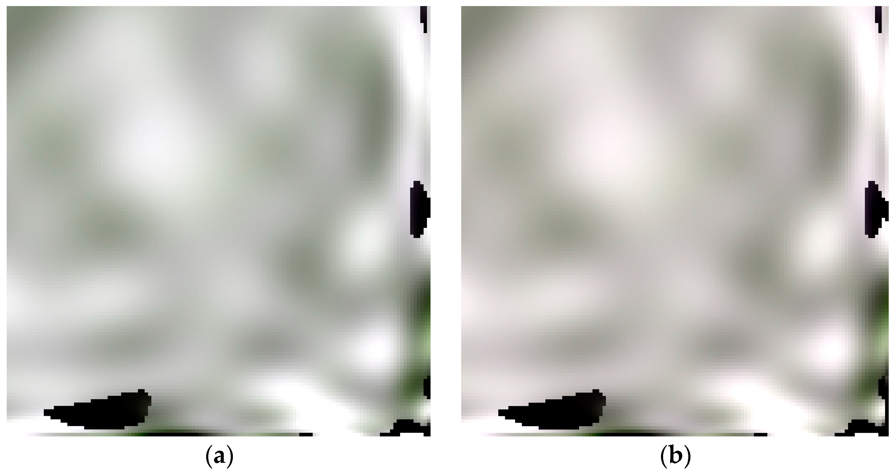
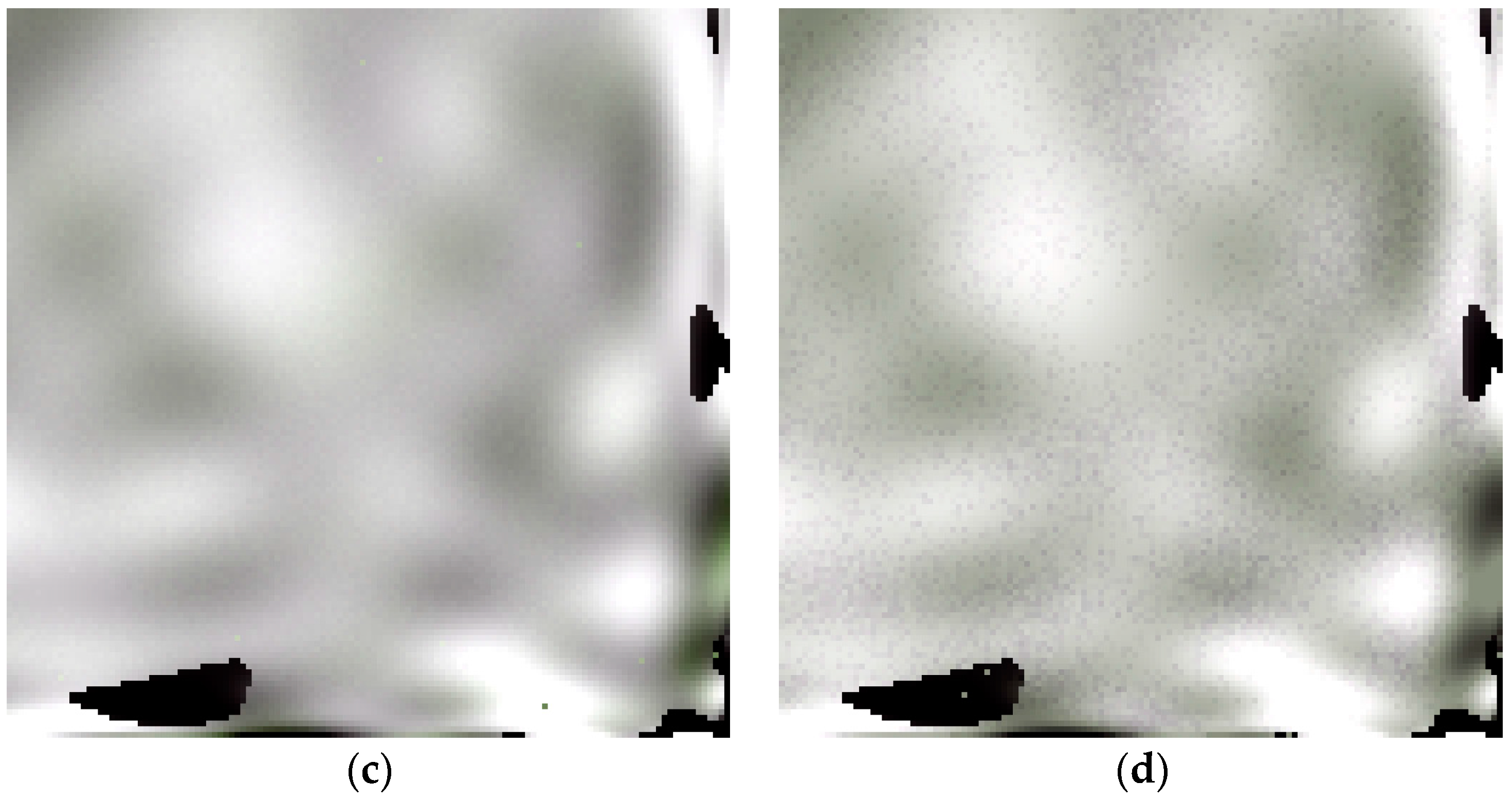
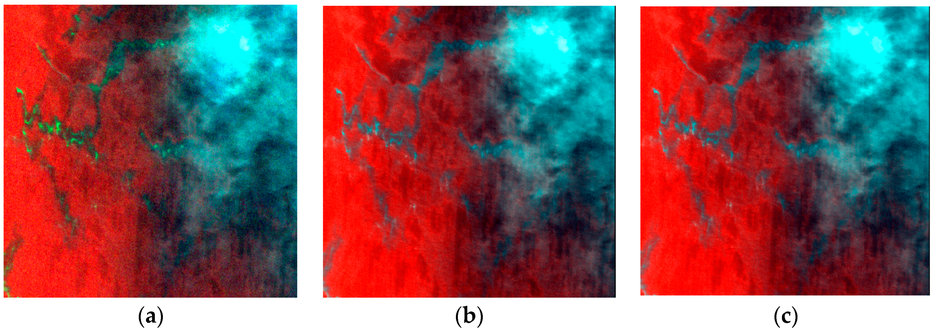
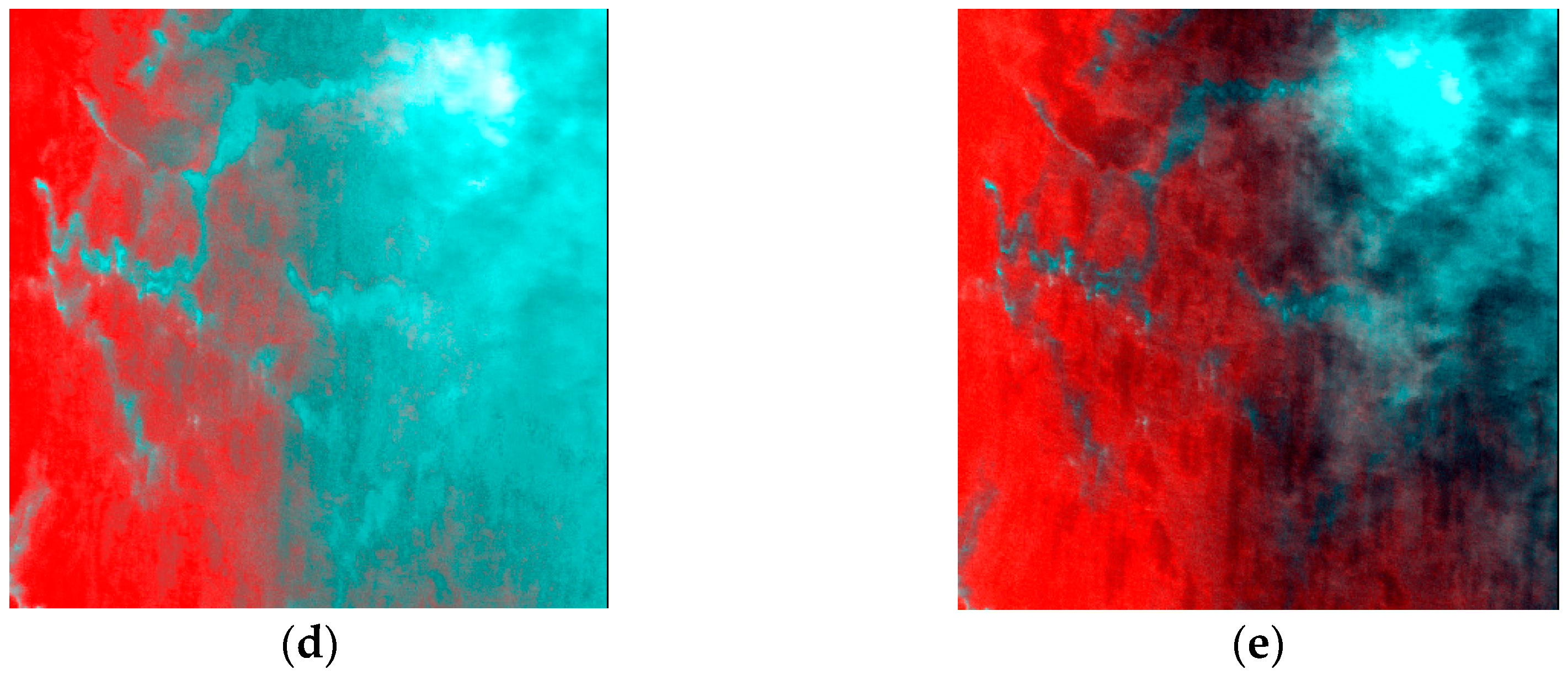
For a more intuitive comparison of the unmixing results using different algorithms, the images were reconstructed by the extracted endmembers and their corresponding abundance. The original hyperspectral images for band 10, band 66, and band 145 are shown in Figure 20, together with the reconstructed images using DSPP+MVSA, SPP+MVSA, RBSPP+MVSA, and SSPP+MVSA.
As shown in Figure 20, the DSPP, SPP, and SSPP combinations exhibited a good performance in terms of endmember extraction. Thus, further quantitative analysis was necessary to compare the preprocessing algorithms. RBSPP could not discriminate the cloud and oil endmembers properly, resulting in a poor reconstruction of thin clouds.
Table 5 tabulates the RMSE values between the original and the reconstructed hyperspectral images. The other algorithms were also optimized for the best performance. As shown in Table 5, the RMSE values using the DSPP algorithm were uniformly low, especially for DSPP+MVSA and DSPP+SISAL. Moreover, the results of the combinations using SPP were also favourable.
We also compared the computational complexity of the proposed DSPP with that of other algorithms using the real hyperspectral images, employing the processing time as our metric. Our results are shown in Table 6.
As shown in Table 6, as the size of the image increases, the advantages of the preprocessing algorithm become visible. The processing time is greatly shortened by directly using endmember extraction algorithms. The DSPP and SSPP are quicker than the other endmember extraction algorithms. In addition, the proposed algorithm has the shortest processing time during the entire endmember extraction.
4. Conclusions
In this paper, a new data field-spectral endmember extraction preprocessing algorithm has been proposed for the identification of marine oil spills. The proposed preprocessing algorithm can extract endmember candidates that could be used prior to subsequent endmember extraction and the spectral unmixing of the hyperspectral images. We applied the algorithms to synthetic hyperspectral images and a real hyperspectral image covering oil films. The extracted endmembers have been used for hyperspectral unmixing using the FCLS method. Using the SSM, RMSE, and processing time as metrics, the proposed algorithm has been shown to be efficient, robust, and fast through a comparison with existing preprocessing algorithms and noise robustness experiments. The proposed algorithm has the advantage of identifying candidates accurately, including anomalous endmembers. Therefore, this is an effective method to monitor oil spills using hyperspectral images. However, the method also has limitations in that it has more input parameters. The identification of an endmember extraction method for hyperspectral unmixing with no additional supervised inputs should be the goal of future research.
Acknowledgments
The authors would like to thank Gabriel Martín and Antonio Plaza for sharing the SPP, RBSPP, and SSPP preprocessing algorithms. This paper was supported by the National Natural Science Foundation of China under Grant No. 41571336 and 51509030.
Author Contributions
Can Cui designed the experiment and procedure; Ying Li performed the experiment; Bingxin Liu analyzed the result; they all wrote the manuscript; Guannan Li made major contributions to the interpretations and modification.
Conflicts of Interest
The authors declare no conflict of interest.
References
- Australian science. Effects of a Crude Oil Spill On Ecology. Available online: http://www.australianscience.com.au/environmental-science/effects-of-a-crude-oil-spill-on-ecology/ (accessed on 7 March 2012).
- Zhao, J.; Temimi, M.; Ghedira, H.; Hu, C. Exploring the potential of optical remote sensing for oil spill detection in shallow coastal waters-a case study in the Arabian Gulf. Opt. Express 2014, 22, 13755–13772. [Google Scholar] [CrossRef] [PubMed]
- Liu, B.; Li, Y.; Chen, P.; Zhu, X. Extraction of oil spill information using decision tree based minimum noise fraction transform. J. Indian Soc. Remote Sens. 2016, 44, 421–426. [Google Scholar] [CrossRef]
- White, H.K.; Conmy, R.N.; MacDonald, I.R.; Reddy, C.M. Methods of oil detection in response to the Deepwater Horizon oil spill. Oceanography 2016, 29, 76–87. [Google Scholar] [CrossRef]
- Mei, S.; He, M.; Zhang, Y.; Wang, Z.; Feng, D. Improving spatial-spectral endmember extraction in the presence of anomalous ground objects. IEEE Trans. Geosci. Remote Sens. 2011, 49, 4210–4222. [Google Scholar] [CrossRef]
- Boardman, J.W.; Kruscl, F.A.; Grccn, R.O. Mapping target signatures via partial unmixing of AVIRIS data. Summaries. In Proceedings of the Fifth JPL Airborne Earth Science Workshop, Pasadena, CA, USA, 23 January 1995; pp. 23–26. [Google Scholar]
- Winter, M.E. N-FINDR: An algorithm for fast autonomous spectral end-member determination in hyperspectral data. In Proceedings of the SPIE’s International Symposium on Optical Science, Engineering, and Instrumentation, Boston, MA, USA, 20–21 September 1999; pp. 266–275. [Google Scholar]
- Harsanyi, J.C.; Chang, C.I. Hyperspectral image classification and dimensionality reduction: An orthogonal subspace projection approach. IEEE Trans. Geosci. Remote Sens. 1994, 32, 779–785. [Google Scholar] [CrossRef]
- Nascimento, J.M.P.; Dias, J.M.B. Vertex component analysis: A fast algorithm to unmix hyperspectral data. IEEE Trans. Geosci. Remote Sens. 2005, 43, 898–910. [Google Scholar] [CrossRef]
- Li, J.; Bioucas-Dias, J.M. Minimum Volume Simplex Analysis: A Fast Algorithm to Unmix Hyperspectral Data. In Proceedings of the 2008 IEEE International Geoscience and Remote Sensing Symposium, IGARSS 2008, Boston, MA, USA, 7–11 July 2008. [Google Scholar] [CrossRef]
- Bioucas-Dias, J.M. A variable splitting augmented Lagrangian approach to linear spectral unmixing. In Proceedings of the 1st International Workshop on Hyperspectral Image and Signal Processing: Evolution in Remote Sensing (WHISPERS 2009), Grenoble, France, 26–28 August 2009. [Google Scholar] [CrossRef]
- Berman, M.; Kiiveri, H.; Lagerstrom, R.; Ernst, A. Ice: A statistical approach to identifying endmembers in hyperspectral images. IEEE Trans. Geosci. Remote Sens. 2008, 42, 2085–2095. [Google Scholar] [CrossRef]
- Ifarraguerri, A.; Chang, C.I. Multispectral and hyperspectral image analysis with convex cones. IEEE Trans. Geosci. Remote Sens. 1999, 37, 756–770. [Google Scholar] [CrossRef]
- Neville, R.; Staenz, K. Automatic endmember extraction from hyperspectral data for mineral exploration. In Proceedings of the 4th International Airborne Remote Sensing Conference and Exhibition/21st Canadian Symposium on Remote Sensing, Ottawa, ON, Canada, 21–24 June 1999. [Google Scholar]
- Plaza, A.; Martinez, P.; Perez, R.; Plaza, J. Spatial/spectral endmember extraction by multidimensional morphological operations. IEEE Trans. Geosci. Remote Sens. 2002, 40, 2025–2041. [Google Scholar] [CrossRef]
- Rogge, D.M.; Rivard, B.; Zhang, J.; Sanchez, A.; Harris, J.; Feng, J. Integration of spatial-spectral information for the improved extraction of endmembers. Remote Sens. Environ. 2007, 110, 287–303. [Google Scholar] [CrossRef]
- Mei, S.; He, M.; Wang, Z.; Feng, D. Spatial purity based endmember extraction for spectral mixture analysis. IEEE Trans. Geosci. Remote Sens. 2010, 48, 3434–3445. [Google Scholar] [CrossRef]
- Zortea, M.; Plaza, A. Spatial preprocessing for endmember extraction. IEEE Trans. Geosci. Remote Sens. 2009, 47, 2679–2693. [Google Scholar] [CrossRef]
- Martin, G.; Plaza, A. Region-based spatial preprocessing for endmember extraction and spectral unmixing. IEEE Geosci. Remote Sens. Lett. 2011, 8, 745–749. [Google Scholar] [CrossRef]
- Martin, G.; Plaza, A. Spatial-spectral preprocessing prior to endmember identification and unmixing of remotely sensed hyperspectral data. IEEE J. Sel. Top. Appl. Earth Obs. Remote Sens. 2012, 5, 380–395. [Google Scholar] [CrossRef]
- Kowkabi, F.; Ghassemian, H.; Keshavarz, A. A fast spatial-spectral preprocessing module for hyperspectral endmember extraction. IEEE Geosci. Remote Sens. Lett. 2016, 13, 782–786. [Google Scholar] [CrossRef]
- Lopez, S.; Moure, J.F.; Plaza, A.; Callico, G.M.; Lopez, J.F.; Sarmiento, R. A new preprocessing technique for fast hyperspectral endmember extraction. IEEE Geosci. Remote Sens. Lett. 2013, 10, 1070–1074. [Google Scholar] [CrossRef]
- Li, D.; Du, Y. Artificial Intelligence with Uncertainty; National Defence Industry Press: Beijing, China, 2005; pp. 198–199. ISBN 9787118039214. [Google Scholar]
- Wu, T.; Qin, K. Image data field for homogeneous region based segmentation. Comput. Electr. Eng. 2012, 38, 459–470. [Google Scholar] [CrossRef]
- Wu, T.; Qin, K. Data field-based transition region extraction and thresholding. Opt. Lasers Eng. 2012, 50, 131–139. [Google Scholar] [CrossRef]
- Franchi, G.; Angulo, J. Morphological principal component analysis for hyperspectral image analysis. ISPRS Int. J. Geo-Inf. 2016, 5, 83, in press. [Google Scholar] [CrossRef]
- Bioucas-Dias, J.M.; Nascimento, J.M.P. Hyperspectral subspace identification. IEEE Trans. Geosci. Remote Sens. 2008, 46, 2435–2445. [Google Scholar] [CrossRef]
- Heinz, D.; Chang, C.I. Fully constrained least squares linear mixture analysis for material quantification in hyperspectral imagery. IEEE Trans. Geosci. Remote Sens. 2001, 39, 529–545. [Google Scholar] [CrossRef]
- Hyperspectral Imagery Synthesis Toolbox for MATLAB. Available online: http://www.ehu.es/ccwintco/index.php/Hyperspectral_Imagery_Synthesis_tools_for_MATLAB (accessed on 5 April 2011).
Figure 1.
Flowchart of the proposed DSPP algorithm.

Figure 2.
Instruction of data field model [23].
Figure 2.
Instruction of data field model [23].

Figure 3.
Simulated image. (a) ; (b) , .

Figure 4.
Data field. (a) ; (b) , .

Figure 5.
Simulated image with anomaly pixels. (a) ; (b) .

Figure 6.
Data field with anomaly pixels. (a) ; (b) .

Figure 7.
Endmember spectra.

Figure 8.
Synthetic hyperspectral scenes.

Figure 9.
Data fields corresponding to different impact factors.

Figure 10.
Endmember candidates-data field.

Figure 11.
Endmember candidates-spectral purity.

Figure 12.
Abundance maps. (a) Water; (b) Oil; (c) Cloud.

Figure 13.
Reconstructed images. (a) DSPP+VCA; (b) SPP+VCA; (c) RBSPP+VCA; (d) SSPP+VCA.


Figure 14.
RMSE between the five reconstructed images and the original images.

Figure 15.
Synthetic image (SNR = 30 dB).

Figure 16.
Comparison of endmembers (SNR = 30 dB) .

Figure 17.
Comparison of the endmembers extracted using several different algorithms and their origins. (a) DSPP+MVSA; (b) SPP+ MVSA; (c) RBSPP+ MVSA; (d) SSPP+ MVSA.
Figure 17.
Comparison of the endmembers extracted using several different algorithms and their origins. (a) DSPP+MVSA; (b) SPP+ MVSA; (c) RBSPP+ MVSA; (d) SSPP+ MVSA.

Figure 18.
The abundance maps using DSPP+MVSA. (a) oil; (b) water; (c) cloud.

Figure 19.
The abundance maps using RBSPP+MVSA. (a) oil (b) water; (c) cloud.

Figure 20.
The reconstructed images obtained using the preprocessing algorithms and MVSA combinations. (a) Original image; (b) DSPP reconstructed image; (c) SPP reconstructed image; (d) RBSPP reconstructed image; (e) SSPP reconstructed image.
Figure 20.
The reconstructed images obtained using the preprocessing algorithms and MVSA combinations. (a) Original image; (b) DSPP reconstructed image; (c) SPP reconstructed image; (d) RBSPP reconstructed image; (e) SSPP reconstructed image.


Table 1.
SSM values of endmembers obtained using different SNRs and several different algorithms.
| SSM | Algorithm | SNR = 30 dB | SNR = 70 dB | SNR = 110 dB | ||||||
|---|---|---|---|---|---|---|---|---|---|---|
| Water | Oil | Clouds | Water | Oil | Clouds | Water | Oil | Clouds | ||
| DSPP | DSPP+VCA | 0.51 | 2.70 | 0.01 | 0.01 | 0.63 | 0.01 | 0.00 | 0.62 | 0.01 |
| DSPP+OSP | 0.02 | 73.02 | 0.11 | 0.00 | 3.58 | 0.02 | 0.00 | 3.67 | 0.02 | |
| DSPP+MVSA | 52.70 | 19.91 | 0.47 | 0.01 | 1.33 | 0.06 | 0.00 | 2.22 | 0.00 | |
| DSPP+SISAL | 0.61 | 23.32 | 0.45 | 1.55 | 1.89 | 0.03 | 0.20 | 2.98 | 0.00 | |
| SPP | SPP+VCA | 39.60 | 23.27 | 0.26 | 31.49 | 25.80 | 0.17 | 27.63 | 0.66 | 0.20 |
| SPP+OSP | 25.37 | 0.63 | 0.15 | 28.70 | 0.74 | 0.22 | 27.33 | 0.65 | 0.23 | |
| SPP+MVSA | 15.83 | 64.15 | 0.09 | 20.45 | 0.67 | 0.00 | 17.65 | 0.79 | 0.03 | |
| SPP+SISAL | 19.00 | 93.31 | 1.04 | 27.33 | 0.92 | 0.00 | 29.64 | 0.53 | 0.01 | |
| RBSPP | RBSPP+VCA | 252.97 | 30.35 | 5.02 | 259.25 | 10.44 | 3.77 | 259.42 | 8.25 | 3.88 |
| RBSPP+OSP | 266.58 | 37.11 | 5.45 | 260.18 | 69.90 | 4.06 | 259.36 | 34.53 | 4.13 | |
| RBSPP+MVSA | 707.84 | 7.70 | 4.42 | 374.27 | 0.28 | 0.40 | 185.37 | 10.59 | 1.61 | |
| RBSPP+SISAL | 114.02 | 44.99 | 4.56 | 196.16 | 9.14 | 0.51 | 187.66 | 10.04 | 1.48 | |
| SSPP | SSPP+VCA | 265.53 | 27.45 | 6.07 | 263.59 | 31.62 | 4.27 | 260.13 | 20.99 | 4.15 |
| SSPP+OSP | 274.70 | 27.91 | 3.82 | 264.28 | 26.87 | 3.50 | 267.71 | 6.15 | 3.65 | |
| SSPP+MVSA | 238.13 | 25.96 | 1.62 | 114.76 | 34.69 | 2.89 | 81.98 | 33.26 | 2.23 | |
| SSPP+SISAL | 231.33 | 27.03 | 1.78 | 133.27 | 35.14 | 3.81 | 104.80 | 33.97 | 3.30 | |
Table 2.
RMSEs of reconstructed images using different SNRs and different algorithms.
| RMSE | Algorithm | SNR = 30 dB | SNR = 70 dB | SNR = 110 dB |
|---|---|---|---|---|
| DSPP | DSPP+VCA | 4.6 | 1.999 | 1.284 |
| DSPP+OSP | 5.14 | 2.43 | 1.61 | |
| DSPP+MVSA | 4.6 | 1.995 | 1.283 | |
| DSPP+SISAL | 4.6 | 1.997 | 1.29 | |
| SPP | SPP+VCA | 4.95 | 3.094 | 2.39 |
| SPP+OSP | 5.17 | 3.085 | 2.54 | |
| SPP+MVSA | 5.07 | 1.975 | 1.426 | |
| SPP+SISAL | 4.58 | 1.976 | 1.29 | |
| RBSPP | RBSPP+VCA | 10.9 | 9.86 | 9.962 |
| RBSPP+OSP | 11.02 | 9.87 | 9.961 | |
| RBSPP+MVSA | 8.94 | 4.03 | 6.46 | |
| RBSPP+SISAL | 9.18 | 4.45 | 6.26 | |
| SSPP | SSPP+VCA | 12.49 | 9.98 | 10.51 |
| SSPP+OSP | 10.04 | 9.88 | 10.05 | |
| SSPP+MVSA | 7.27 | 7.49 | 6.72 | |
| SSPP+SISAL | 7.49 | 8.48 | 7.99 |
Table 3.
Processing time comparisons using different algorithms.
| Algorithm | Preprocessing Time (s) | Endmember Extraction Time (s) | Total Time (s) | |
|---|---|---|---|---|
| ORIGINAL | VCA | \ | 60.26 | 50.26 |
| OSP | \ | 136.87 | 136.87 | |
| MVSA | \ | 350.42 | 350.42 | |
| SISAL | \ | 172.52 | 172.52 | |
| DSPP | DSPP+VCA | 63.28 | 9.24 | 72.52 |
| DSPP+OSP | 63.28 | 10.86 | 74.14 | |
| DSPP+MVSA | 63.28 | 241.4 | 304.68 | |
| DSPP+SISAL | 63.28 | 8.31 | 71.59 | |
| SPP | SPP+VCA | 56.54 | 48.88 | 105.42 |
| SPP+OSP | 56.54 | 128.95 | 185.49 | |
| SPP+MVSA | 56.54 | 342.35 | 398.89 | |
| SPP+SISAL | 56.54 | 163.25 | 219.79 | |
| RBSPP | RBSPP+VCA | 83.71 | 8.69 | 92.4 |
| RBSPP+OSP | 83.71 | 9.98 | 93.69 | |
| RBSPP+MVSA | 83.71 | 256.8 | 340.51 | |
| RBSPP+SISAL | 83.71 | 9.05 | 92.76 | |
| SSPP | SSPP+VCA | 69.52 | 5.85 | 75.37 |
| SSPP+OSP | 69.52 | 6.72 | 76.24 | |
| SSPP+MVSA | 69.52 | 244.09 | 313.61 | |
| SSPP+SISAL | 69.52 | 8.58 | 78.1 |
Table 4.
SSM value of endmembers using several different algorithms.
| SSM | Algorithm | Water | Oil | Clouds |
|---|---|---|---|---|
| DSPP | DSPP+VCA | 0.0042 | 1.3083 | 0.5910 |
| DSPP+OSP | 0.1352 | 3.8199 | 0.5078 | |
| DSPP+MVSA | 0.3702 | 1.4977 | 2.0667 | |
| DSPP+SISAL | 0.5281 | 0.9696 | 2.5910 | |
| SPP | SPP+VCA | 0.0299 | 1.3041 | 1.054 |
| SPP+OSP | 0.0288 | 3.2215 | 1.2586 | |
| SPP+MVSA | 0.0952 | 0.7771 | 2.9965 | |
| SPP+SISAL | 0.0608 | 0.7013 | 1.9358 | |
| RBSPP | RBSPP+VCA | 0.3898 | 3.5866 | 6.6255 |
| RBSPP+OSP | 1.6857 | 4.2385 | 6.26 | |
| RBSPP+MVSA | 0.6622 | 2.5833 | 4.1918 | |
| RBSPP+SISAL | 1.2356 | 3.7815 | 2.4958 | |
| SSPP | SSPP+VCA | 0.0187 | 1.1604 | 3.0309 |
| SSPP+OSP | 0.0243 | 0.6502 | 2.5849 | |
| SSPP+MVSA | 0.0976 | 2.6116 | 4.9067 | |
| SSPP+SISAL | 0.102 | 2.2873 | 6.3993 |
Table 5.
RMSE values between the original and the reconstructed hyperspectral images using different algorithms.
Table 5.
RMSE values between the original and the reconstructed hyperspectral images using different algorithms.
| Algorithm | RMSE | |
|---|---|---|
| DSPP | DSPP+VCA | 4.820846 |
| DSPP+OSP | 8.338002 | |
| DSPP+MVSA | 3.127129 | |
| DSPP+SISAL | 3.147139 | |
| SPP | SPP+VCA | 4.097042 |
| SPP+OSP | 5.150471 | |
| SPP+MVSA | 3.136146 | |
| SPP+SISAL | 3.153928 | |
| RBSPP | RBSPP+VCA | 6.02655 |
| RBSPP+OSP | 8.232756 | |
| RBSPP+MVSA | 3.915835 | |
| RBSPP+SISAL | 4.212568 | |
| SSPP | SSPP+VCA | 5.620443 |
| SSPP+OSP | 8.221507 | |
| SSPP+MVSA | 3.187329 | |
| SSPP+SISAL | 3.312629 |
Table 6.
Processing time comparisons using different algorithms.
| Algorithm | Preprocessing Time (s) | Endmember Extraction Time (s) | Total Time (s) | |
|---|---|---|---|---|
| ORIGINAL | VCA | \ | 472.52 | 472.52 |
| OSP | \ | 650.42 | 650.42 | |
| MVSA | \ | 20,254.52 | 20,254.52 | |
| SISAL | \ | 828.86 | 828.86 | |
| DSPP | DSPP+VCA | 138.85 | 160.87 | 299.72 |
| DSPP+OSP | 138.85 | 174.41 | 313.26 | |
| DSPP+MVSA | 138.85 | 1587.35 | 1726.2 | |
| DSPP+SISAL | 138.85 | 168.25 | 307.1 | |
| SPP | SPP+VCA | 119.23 | 489.25 | 608.48 |
| SPP+OSP | 119.23 | 508.28 | 627.51 | |
| SPP+MVSA | 119.23 | 20073.1 | 20,192.33 | |
| SPP+SISAL | 119.23 | 756.35 | 875.58 | |
| RBSPP | RBSPP+VCA | 173.21 | 175.65 | 348.86 |
| RBSPP+OSP | 173.21 | 165.91 | 339.12 | |
| RBSPP+MVSA | 173.21 | 1640.92 | 1814.13 | |
| RBSPP+SISAL | 173.21 | 153.47 | 326.68 | |
| SSPP | SSPP+VCA | 152.68 | 163.89 | 316.57 |
| SSPP+OSP | 152.68 | 168.01 | 320.69 | |
| SSPP+MVSA | 152.68 | 1610.68 | 1763.36 | |
| SSPP+SISAL | 152.68 | 175.24 | 327.92 |
© 2017 by the authors. Licensee MDPI, Basel, Switzerland. This article is an open access article distributed under the terms and conditions of the Creative Commons Attribution (CC BY) license (http://creativecommons.org/licenses/by/4.0/).
Share and Cite
MDPI and ACS Style
Cui, C.; Li, Y.; Liu, B.; Li, G. A New Endmember Preprocessing Method for the Hyperspectral Unmixing of Imagery Containing Marine Oil Spills. ISPRS Int. J. Geo-Inf. 2017, 6, 286. https://doi.org/10.3390/ijgi6090286
AMA Style
Cui C, Li Y, Liu B, Li G. A New Endmember Preprocessing Method for the Hyperspectral Unmixing of Imagery Containing Marine Oil Spills. ISPRS International Journal of Geo-Information. 2017; 6(9):286. https://doi.org/10.3390/ijgi6090286
Chicago/Turabian StyleCui, Can, Ying Li, Bingxin Liu, and Guannan Li. 2017. "A New Endmember Preprocessing Method for the Hyperspectral Unmixing of Imagery Containing Marine Oil Spills" ISPRS International Journal of Geo-Information 6, no. 9: 286. https://doi.org/10.3390/ijgi6090286
Note that from the first issue of 2016, this journal uses article numbers instead of page numbers. See further details here.