Robust Hessian Locally Linear Embedding Techniques for High-Dimensional Data

Abstract

Recently manifold learning has received extensive interest in the community of pattern recognition. Despite their appealing properties, most manifold learning algorithms are not robust in practical applications. In this paper, we address this problem in the context of the Hessian locally linear embedding (HLLE) algorithm and propose a more robust method, called RHLLE, which aims to be robust against both outliers and noise in the data. Specifically, we first propose a fast outlier detection method for high-dimensional datasets. Then, we employ a local smoothing method to reduce noise. Furthermore, we reformulate the original HLLE algorithm by using the truncation function from differentiable manifolds. In the reformulated framework, we explicitly introduce a weighted global functional to further reduce the undesirable effect of outliers and noise on the embedding result. Experiments on synthetic as well as real datasets demonstrate the effectiveness of our proposed algorithm.

1. Introduction

Over the past 10 years, manifold learning has become a significant component of pattern recognition, machine learning, computer vision and robotics. A large number of nonlinear manifold learning methods have been proposed to discover the intrinsic structures of high-dimensional datasets, including Isometric feature mapping [1], Locally Linear Embedding (LLE) [2], Laplacian Eigenmaps (LE) [3], Local Tangent Space Alignment (LTSA) [4], Hessian eigenmaps or HLLE [5], Maximum Variance Unfolding (MVU) [6], Riemannian Manifold learning [7], Maximal linear embedding [8] and Fusion of Local Manifold learning methods (FLM) [9]. The discovered low-dimensional structures can be further used for classification, clustering, and data visualization. Most manifold learning algorithms assume that the sampled high-dimensional data reside on a smooth low-dimensional manifold. The basic manifold assumption [10] is also the key assumption in manifold classification [11,12] and manifold clustering [13]. However, the basic assumption may be unsuitable for real applications since real-world data are often contaminated with outliers and noises due to human mistakes or imperfect sensors. Outliers are observations that deviate so much from the underlying manifold as to arouse suspicion that they were generated by a different mechanism [14]. The percentage of outliers in the whole dataset is usually small. Comparing to outliers, noises are observations that deviate a little from the underlying manifold, while the percentage of noises can be large. Outliers and noises puzzle the existing manifold learning algorithms; therefore, a robust design is important to extend manifold learning to more realistic and challenging applications.

Some extensions have been proposed to improve the robustness of existing manifold learning algorithms. Chang and Yeung [15] attempt to address the outlier problem by proposing a robust version of LLE. RLLE adopts robust principal component analysis (RPCA) [16] to estimate the reliability score of each data point, then uses these reliable scores to detect outliers. Zhan and Yin [17] address this problem in the context of LTSA. RLTSA first performs RPCA to obtain local tangent coordinates; then using the result of RPCA, RLTSA minimizes the weighted local alignment error to obtain embedding result. Although some experimental results show that RLLE and RLTSA are robust against outliers, they still have some disadvantages: RPCA uses an iterative procedure to find the solution by starting from some estimates which is time consuming for high-dimensional data. Moreover, RLLE and RLTSA would fail when the dataset is corrupted by a large amount of small noises [18]. Zhang and Zha [18,19] propose a local smooth method for noise reduction. It is based on a weighted version of PCA to regulate the input data locally. Although this procedure is efficient for noisy data, it is not suitable for outliers. Since pulling back the outliers requires multiple iterations, the local-smoothing procedure suffers from the “trim the peak and fill the valley” phenomenon for regions of the manifold where the curvature is large. Hein and Maier [20] present a manifold denoising algorithm based on a graph-based diffusion process of the point sample. The denoising algorithm can be used as a pre-processing step to improve the discriminative capacity of graph-based semi-supervised learning [21,22]. However, since the diffusion process on the graph may concentrate the data into local clusters and change the local geometric structures of the original data, manifold denoising is not suitable for faithfully recovering the low-dimensional embedding. More recently, Gashler and Martinez [23] proposed a robust manifold learning method called CycleCut which is inspired by max-flow/min-cut methods for graph partitioning. The CycleCut algorithm can remove short-circuit connections and sever toroidal connections in a manifold. However, CycleCut cannot improve the stabilization of manifold learning algorithms, which means that CycleCut would also fail when the data have large amounts of small noises.

To our best knowledge, however, there is no extension of HLLE to address the outlier or noise problem. In this paper, we investigate the robust manifold learning problem in the context of HLLE and propose a robust version of HLLE algorithm called RHLLE. It is worthwhile to highlight our main contributions here:

(1)

We reformulate the original HLLE algorithm through the truncation function from differential manifold [24]. As far as we know, we are the first to explicitly relate the truncation function from differential manifold to a classical manifold learning method, i.e., HLLE, to explain the connection between the local geometric object and the global geometric object of the manifold. With the help of this reformulation, we explicitly propose a weighted global functional to reduce the influence of outliers and noises.

(2)

We propose a fast outlier detection method based on robust statistics [25]. In contrast to the traditional RPCA-based algorithms, our method is much more efficient for high-dimensional datasets. Our proposed method can be successfully applied to the existing manifold learning algorithms to improve their robustness.

(3)

As reviewed in this section, the related works are suitable for either the outlier or noise problem. In contrast, our RHLLE algorithm is robust against both outliers and noises.

The rest of the paper is organized as follows: we first briefly review the original HLLE algorithm and reformulate it through the truncation function from the differential manifold in Section 2. The sensitivity of HLLE to outliers and noises is illustrated in Section 3. Section 4 gives the details of our proposed RHLLE algorithm. Experimental results are reported in Section 5 and Section 6 concludes.

2. Reformulating HLLE through Truncation Function from Differential Manifold

2.1. Brief Review of Hessian LLE

Hessian LLE may be viewed as a modification of locally-linear embedding and its theoretical framework as a modification of the Laplacian eigenmap framework by replacing the Laplacian operator with the Hessian. HLLE is guaranteed to asymptotically recover the true manifold if the manifold is locally isometric to an open connected subset of ${\mathbb{R}}^d$ [5].

Consider a dataset X, which consists of N data points $x_1,x_2,\cdots ,x_N$ in high-dimensional space ${\mathbb{R}}^D$, and hypothesize that they lie on a smooth manifold $\mathcal{M}\subset {\mathbb{R}}^D$ of intrinsic dimensionality $d<D$. Let $X=[x_1,x_2,\cdots ,x_N]\in {\mathbb{R}}^{D\times N}$ and $Y=[y_1,y_2,\cdots ,y_N]\in {\mathbb{R}}^{d\times N}$ denote the matrix of all sampled points and their embedding coordinates, respectively. The objective of a manifold-based dimensionality reduction algorithm is to recover the corresponding low-dimensional coordinates $y_i\in \mathcal{Y}$ of each $x_i\in \mathcal{M}$. In other words, we assume $\mathcal{M}$ is the image of some coordinate space $\mathcal{Y}\subset {\mathbb{R}}^d$ under some smooth mapping $\psi :\mathcal{Y}\to {\mathbb{R}}^D$. Because the mapping ψ is a locally-isometric embedding, the inverse mapping $\varphi ={\psi }^{-1}:\mathcal{M}\to {\mathbb{R}}^d$ provides a locally-isometric coordinate system on $\mathcal{M}$. Let x be a fixed point in the interior of $\mathcal{M}$, and $T_x(\mathcal{M})$ be the tangent space defined at x. To define the Hessian, HLLE uses the orthogonal coordinates on the tangent space to compute the Hessian of a function $f:\mathcal{M}\to \mathbb{R}$ that is $C^2$ near x. Suppose that the tangent coordinate of $x\in \mathcal{N}(x)$ is given by u, where $\mathcal{N}(x)$ is the local patch built by the point x and its k nearest neighborhoods, $\mathcal{N}(x)=\{x,x_1,\cdots ,x_k\}$. Then the rule $g(u)=f(x)=f\circ \psi (u)$ defines a function $g:U\to \mathbb{R}$, where U is the neighborhood of $u\in {\mathbb{R}}^d$ formed by the tangent coordinates of $N(x)$. The Hessian of f at x in tangent coordinates can be defined as the ordinary Hessian of g:

$${(H_f^{tan})}_{i,j}(x)=\frac{\partial }{\partial u_i}\frac{\partial }{\partial u_j}g(u){|}_{u=\varphi (x)}$$

(1)

Although different local coordinate systems give different tangent Hessians, all of these Hessians share the same Frobenius norm $\parallel H_f^{tan}{(x)\parallel }_F^2$, so that the following quadratic form can be well defined:

$$\mathcal{H}(f)={\int }_{\mathcal{M}}{\parallel H_f^{tan}(x)\parallel }_F^{2}dx$$

(2)

where $dx$ stands for the canonical measure corresponding to the volume form on $\mathcal{M}$. The functional $\mathcal{H}(f)$ measures the average curviness of f over the manifold $\mathcal{M}$.

The key result of Donoho and Grimes [5] is that, if $\mathcal{M}$ truly is locally-isometric to an open connected subset of ${\mathbb{R}}^d$, then $\mathcal{H}(f)$ has a $(d+1)$-dimensional null space, consisting of the constant functions and a d-dimensional space of functions spanned by the original isometric coordinates. The HLLE algorithm adapts the basic structure of LLE to estimate the nullspace of the functional $\mathcal{H}(f)$, and has five steps:

(1)

Find nearest neighbors: For each data point $x_i$, find the indices corresponding to the k-nearest neighbors in Euclidean distance. Let $\mathcal{N}(x_i)$ denote the collection of those neighbors.

(2)

Obtain tangent coordinates: Perform a singular value decomposition on the points in $\mathcal{N}(x_i)$, getting their tangent coordinates.

(3)

Develop Hessian estimator: Develop the infrastructure for least-squares estimation of the local Hessian operator $H^i$.

(4)

Develop quadratic form: Build a symmetric matrix $\overline{\mathcal{H}}$ having, in coordinate pair $ij$, the entry ${\overline{\mathcal{H}}}_{i,j}={\sum }_l{\sum }_r({(H^l)}_{r,i}{(H^l)}_{r,j})$. $\overline{\mathcal{H}}$ approximates the continuous operator $\mathcal{H}$.

(5)

Compute the embedding from the estimated $\mathcal{H}$ functional: Perform an eigenanalysis of $\overline{\mathcal{H}}$ and choose Y to be the eigenvectors corresponding to the d smallest eigenvalues, excluding the constant eigenvector.

2.2. Reformulating Hessian LLE

The original implementation of HLLE lacks a straightforward interpretation about the construction of the approximated Hessian functional $\overline{\mathcal{H}}$ in Step 4. The original implementation also lacks an unambiguous explanation about the estimation of the local Hessian operator $H^i$ in Step 3. Furthermore, it is time consuming to use SVD to compute the tangent coordinates for the high-dimensional data. In this subsection, we present an alternative way to formulate HLLE. The truncation function from differential manifold [24] is employed for relating the locality and the global structure of the manifold. In the given framework, a straightforward interpretation about the construction of the approximated Hessian functional explicitly appears. For completeness, we also give an unambiguous explanation about the estimation of the local Hessian operator and the tangent coordinates in this subsection. It is worth noting that Kim et al. [26] also propose a similar way to estimate the Hessian energy using the local tangent coordinates in the context of semi-supervised regression. The proposed work is focused on the context of dimensionality reduction while the work in [26] is focused on the context of semi-supervised regression. The essence of the two works in the estimation of the local Hessian operator and the tangent coordinates is the same. However, our expression and formulation is easier to follow. Recently, based on the local tangent coordinates, Lin et al. [27,28] proposed a parallel vector field approach to approximate a second order operator, the connection Laplacian, which can also be used to approximate the Hessian operator.

In order to estimate the local tangent coordinates, we first perform PCA on the points in $\mathcal{N}(x_i)$ and get d leading PCA eigenvectors $V^i=\{v_1^i,v_2^i,\cdots ,v_d^i\}$, which correspond to an orthogonal basis of $T_{x_i}(\mathcal{M})$ (seen as a d-dimensional affine subspace of ${\mathbb{R}}^D$ that is tangent to $\mathcal{M}$ at $x_i$). The trick presented by Turk and Pentland for EigenFaces [29] is employed for high-dimensional data. Then the local tangent coordinates ${\{u_j^i\}}_{j=1}^k$ of a point $x_i\in \mathcal{N}(x_i)$ can be computed by projecting the local neighborhoods to this tangent subspace:

$$u_j^i=\langle V^i,x_j-x_i\rangle ={(V^i)}^T(x_j-x_i)$$

(3)

It is worth noting that we fix the origin of the tangent space at $x_i$ to be the data sample itself, while the original algorithm uses the mean of the neighborhood $\mathcal{N}(x_i)$ of $x_i$ to be the origin of the tangent space. When the dataset is non-uniformly distributed or sparse, it is lack of enough data samples to form different neighborhoods in some regions. Therefore, the local tangent spaces computed for the data samples in these regions will become the same. As a consequence, the tangent coordinates of the data samples will be biased. According to [30], the above correction of the origin of the tangent space can overcome the drawbacks of tangent space approximation in dealing with sparse or non-uniformly distributed-data-manifolds.

In order to estimate the local Hessian operator, we first perform a second-order Taylor expansion at a fixed $x_i$ on the smooth functions: ${\{f(x_j)\}}_{j=1}^k,f:\mathcal{M}\to \mathbb{R}$ that is $C^2$ near $x_i$.

$$f(x_j)=f(x_i)+{(\nabla f)}^T(x_j-x_i)+\frac{1}{2}{(x_j-x_i)}^T{H}_f^i(x_j-x_i)+O(\parallel x_j-x_i{\parallel }^3)$$

(4)

Recall that we have defined a function $g:U\to \mathbb{R}$ which uses the local tangent coordinates and satisfies the rule $g(u)=f(x)=f\circ \psi (u)$ in Section 2.1. Together with $u_i^i=\langle V^i,x_i-x_i\rangle =0$, we have:

$$f(x_j)=g(u_j^i)=g(0)+{(\nabla g)}^T{u}_j^i+\frac{1}{2}{u_j^i}^T{H}_f^i{u}_j^i+O(\parallel u_j^i{\parallel }^3)$$

(5)

Over the neighborhood of $u_j^i$, we develop the operator $b^i$ that approximates the function $g(u_j^i)$ by its projection on the basis $U_j^i=\{1,u_{j_1}^i,\cdots ,u_{j_d}^i,{(u_{j_1}^i)}^2,\cdots ,{(u_{j_d}^i)}^2,\cdots ,u_{j_1}^i\times u_{j_2}^i,\cdots ,u_{j_{d-1}}^i\times u_{j_d}^i\}$, we have:

$$f(x_j)=g(u_j^i)={(b^i)}^T·U_j^i$$

(6)

Let $b^i=[g(0),\nabla g,h^i]\in {\mathbb{R}}^{1+d+d(d+1)/2}$; then, $h^i\in {\mathbb{R}}^{d(d+1)/2}$ is the vector form of local Hessian matrix $H_f^i$ over neighborhood $N(x_i)$. The least-squares estimation of the operator $b^i$ can be obtained by:

$$\underset{b^i}{argmin}\sum _{j=1}^k{(f(x_j)-\langle b^i,U_j^i\rangle )}^2$$

(7)

The least-squares solution is $b^i={(U^i)}^{†}{f}^i$, where $f^i=[f(x_1),\cdots ,f(x_k)]\in {\mathbb{R}}^k$, $U^i=[U_1^i;U_2^i;\cdots ;U_k^i]\in {\mathbb{R}}^{k\times (1+d+d(d+1)/2)}$ and ${(U^i)}^{†}$ denotes the pseudo-inverse of $U^i$. Note that the the last $d(d+1)/2$ components of $b^i$ correspond to $h^i$, which is the vector form of local Hessian matrix $H_f^i$. The local Hessian operator $H^i\in {\mathbb{R}}^{(d(d+1)/2)\times k}$ is constructed by the last $d(d+1)/2$ rows of ${(U^i)}^{†}$, and we have: $h^i=H^i·f^i$. Therefore, the local quadratic form $\parallel H_f^{tan}(x_i){\parallel }_F^2$ can be estimated with:

$$\parallel H_f^{tan}(x_i){\parallel }_F^2={(h^i)}^T(h^i)={(f^i)}^T{(H^i)}^T(H^i)(f^i)$$

(8)

$\parallel H_f^{tan}(x_i){\parallel }_F^2$ is a local object defined on the manifold, while $\mathcal{H}(f)$ is a global object defined on the manifold. We use the truncation function from the differential manifold to connect them together. The truncation function is an important tool in the differential manifold to establish a relationship between the local and global properties of the manifold. Suppose U and V are two nonempty subsets of a smooth manifold $\mathcal{M}$, where $\overline{V}$ is compact and $\overline{V}\subset U$ ($\overline{V}$ is the closure of V). Then the truncation function [24] is defined as a smooth function $s:\mathcal{M}\to \mathbb{R}$ such that:

$$s(p)=\left\{\begin{array}{cc}1,\hfill & p\in V\hfill \\ 0,\hfill & p\notin U\hfill \end{array}\right.$$

(9)

The truncation function s can be discretely approximated by the 0-1 selection matrix $S^i\in {\mathbb{R}}^{N\times k}$ and an entry of $S^i$ is defined as:

$${(S^i)}_{pq}=\left\{\begin{array}{cc}1,\hfill & p=N_i\{q\}\hfill \\ 0,\hfill & p\ne N_i\{q\}\hfill \end{array}\right.$$

(10)

where $N_i=\{i_1,\cdots ,i_k\}$ denotes the set of indices for the k-nearest neighborhood of data point $x_i$. Thus, the local object $f^i=[f(x_1^i),\cdots ,f(x_k^i)]\in {\mathbb{R}}^k$ can be expressed by $f^i={(S^i)}^{T}f$, where $f=[f(x_1),\cdots ,f(x_N)]\in {\mathbb{R}}^N$ is a global object defined on the whole manifold.

By using the truncation function and its discrete approximation, together with Equation (8), the global functional $\mathcal{H}$ can be discretely approximated as follows:

$$\begin{array}{cc}\hfill \mathcal{H}(f)& ={\int }_{\mathcal{M}}\parallel H_f^{tan}{(x)\parallel }_F^{2}dx=\frac{1}{N}\sum _{i=1}^N{\parallel H_f^{tan}(x_i)\parallel }_F^2\hfill \\ & =\frac{1}{N}\sum _{i=1}^N{(f^i)}^T{(H^i)}^T(H^i)(f^i)=\frac{1}{N}\sum _{i=1}^N{f}^T{S}^i{(H^i)}^T(H^i){(S^i)}^{T}f\hfill \\ & =f^T\overline{\mathcal{H}}f\hfill \end{array}$$

(11)

where $\overline{\mathcal{H}}=\frac{1}{N}{\sum }_{i=1}^N{S}^i{(H^i)}^T(H^i){(S^i)}^T\in {\mathbb{R}}^{N\times N}$ is a sparse $N\times N$ matrix which approximates the continuous operator $\mathcal{H}$. $\overline{\mathcal{H}}$ is also named alignment matrix in the algorithm of local tangent space alignment (LTSA) [4] and can be computed based on an iterative procedure:

$$\overline{\mathcal{H}}(N_i,N_i)\leftarrow \overline{\mathcal{H}}(N_i,N_i)+{(H^i)}^T(H^i)$$

(12)

where $i=1,\cdots ,N$ and $\overline{\mathcal{H}}$ is initialized by the zero matrix. Recall that $N_i$ is the neighborhood index set with respect to the i-th point.

The global embedding coordinates $Y=[y_1,y_2,\cdots ,y_N]\in {\mathbb{R}}^{d\times N}$ can be obtained by minimizing the functional $\mathcal{H}(f)$. Let $y=f=[f(x_1),\cdots ,f(x_N)]$ be a row vector of Y. It is not hard to know that the embedding coordinates matrix Y is constructed with the eigenvectors corresponding to the d smallest eigenvalues, excluding the constant eigenvector, of $\overline{\mathcal{H}}$.

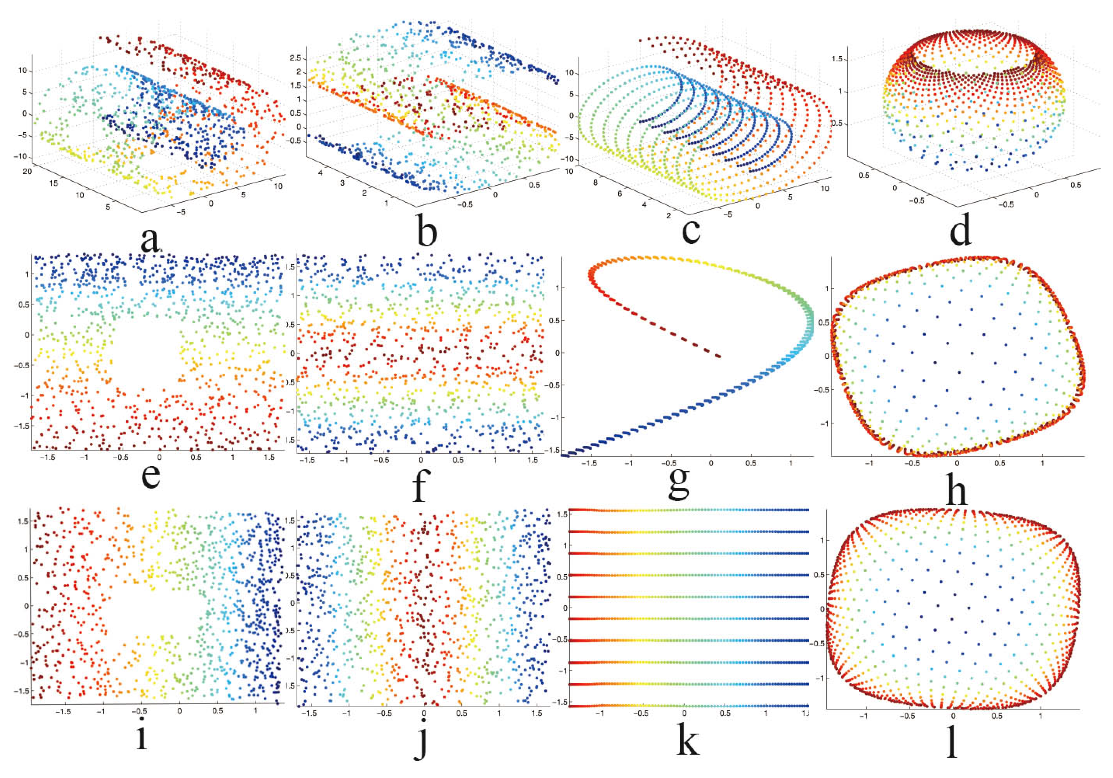
At the end of this section, we compare the original HLLE with our reformulated HLLE on four synthetic 2D manifolds. As we can see from Figure 1, the results derived by both methods are very similar on the ”Swiss Roll with hole” and “S-curve” manifolds, and our reformulated HLLE performs better than the original HLLE on the “Uniform Swiss Roll” and “Punched Sphere” manifolds. The results show that our reformulated HLLE is equivalent to the original HLLE on the general situation, while our reformulated HLLE is superior to the original HLLE in the case when data samples are sparse or not evenly distributed. The reason behind this good performance is that we correct the origin of the tangent space at a point $x_i$ from the mean of the neighborhood of $x_i$ to the point $x_i$ itself. This phenomenon is consistent with the research result of [30] because the local tangent spaces at sparse or not evenly-distributed regions, where there is a lack of data samples to form different neighborhoods, will become the same for two data points that are not adjacent to each other, if one uses the mean of the neighborhood of $x_i$(other than $x_i$ itself) to be the origin of the tangent space.

3. Sensitivity of Hessian LLE to Outliers and Noise

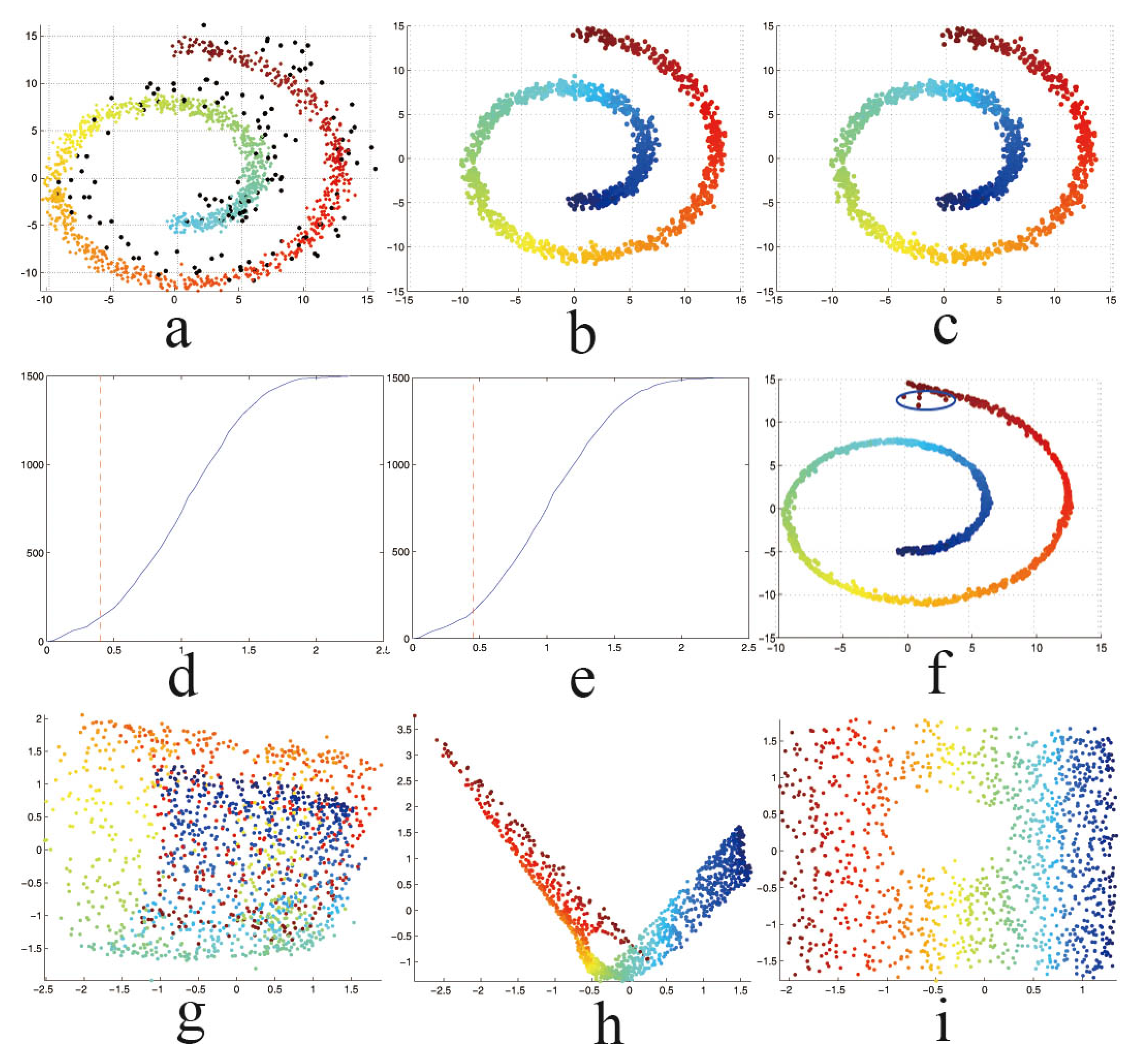
In this section, we use the “Swiss Roll with hole” dataset to illustrate how the HLLE result can be affected by outliers and noises in the data. There are 1500 samples in the dataset. We randomly select 150 samples ($10\%$) and impose uniformly-distributed random noise with a large amplitude on them as outliers. We add Gaussian noise to the remaining $90\%$ of the samples to simulate noise-corrupted data. Figure 2a plots these sample points, where the black points are the outliers and the colored points are the noise-corrupted data. As we can see from Figure 2g, due to outliers and noise, HLLE cannot recover the manifold structure well. In fact, the outliers and noise-corrupted points usually deviate from the smooth surface of the underlying manifold. Therefore, the dimension of the approximated local tangent space of the data points corrupted by the outliers or noises may be larger than the intrinsic dimension of the real manifold. Furthermore, the orientation of the approximated local tangent space of of the data points corrupted by the outliers or noise may deviate from the true one of the local manifold. As a result, the estimated local tangent space cannot catch the real local geometry of the manifold; hence, the local Hessian matrix, which uses the local tangent coordinates cannot reflect the local manifold structure well, leading to a large bias with respect to the true embedding result. Based on robust statistics, the RLLE algorithm can identify and remove the outliers successfully (see Figure 2b). However, RLLE would fail when the data have a large amount of small noises (see Figure 2h). In the next section, we present an approach to make HLLE more robust against both outliers and noises.

4. Robust Hessian Locally Linear Embedding

4.1. Robust PCA

In the original HLLE algorithm, the local tangent coordinates are obtained by performing PCA on each local patch. However, as is well known, PCA is quite sensitive to outliers. An iteratively-reweighted PCA algorithm, called Robust PCA (RPCA) [31], has been proposed to make PCA less sensitive to outliers. The optimization objective for the weighted PCA on the neighborhoods of $x_i$ can be expressed as:

$$min\sum _{j=1}^k{w}_j^i\parallel {\epsilon }_j^i{\parallel }^2=\underset{c^i,{(U^i)}^T{U}^i=I_d}{argmin}\sum _{j=1}^k{w}_j^i{\parallel x_j^i-c^i-U^i{(U^i)}^T(x_j^i-c^i)\parallel }^2$$

(13)

where $U^i\in {\mathbb{R}}^{D\times d}$ forms the orthonormal basis of the local tangent space of the point $x_i$, $c^i\in {\mathbb{R}}^D$ gives the displacement of the local tangent space, and the weights $w_j^i(j=1,2,\cdots ,k)$ are fixed. The least squares solution of the problem is given by:

$$U^i=[u_1^i,\cdots ,u_k^i],c^i=\frac{{\sum }_{j=1}^k{w}_j^i{x}_j^i}{{\sum }_{j=1}^k{w}_j^i}={\overline{x}}_w$$

(14)

where $\{u_1^i,\cdots ,u_k^i\}$ are the eigenvectors of the weighted sample covariance matrix:

$$S_w=\frac{1}{k}\sum _{j=1}^k{w}_j^i(x_j^i-{\overline{x}}_w){(x_j^i-{\overline{x}}_w)}^T$$

(15)

Following the basic ideas from robust statistics, Robust PCA determines the weights $w_j^i$ by the corresponding projection error ${\epsilon }_j^i$:

$$w_j^i=\left\{\begin{array}{cc}1,\hfill & {\epsilon }_j^i\le \frac{1}{2}\overline{{\epsilon }^i}\hfill \\ \frac{\overline{{\epsilon }^i}}{2{\epsilon }_j^i},\hfill & {\epsilon }_j^i>\frac{1}{2}\overline{{\epsilon }^i}\hfill \end{array}\right.$$

(16)

where $\overline{{\epsilon }^i}=\frac{1}{k}{\sum }_{k=1}^1{\epsilon }_j^i$ is the mean value of the projection error of the k nearest neighbors of $x_i$. Then RPCA uses an iterative procedure to find the solution by starting from some initial estimates. The iterative procedure of RPCA can be summarized as follows [32]:

(1)

Perform PCA to compute the orthonormal basis matrix $U^i$ and displacement $c^i$ of the local tangent space. Set $l=0$.

(2)

Repeat until convergence:

(a)

Compute ${({\epsilon }_j^i)}^l=x_j^i-{(c^i)}^l-{(U^i)}^l{{(U^i)}^l}^T(x_j^i-{(c^i)}^l)$;

(b)

Compute ${(w_j^i)}^l(j=1,\cdots ,k)$ according to (16), where ${\epsilon }_j^i={({\epsilon }_j^i)}^l$

(c)

Compute the weighted least squares estimates ${(U^i)}^{(l+1)}$ and ${(c^i)}^{(l+1)}$ according to (14 15), where $w_j^i={(w_j^i)}^l$

(d)

if $\parallel {(U^i)}^{(l+1)}-{(U^i)}^l{\parallel }_F<ϵ$, return;

else $l=l+1$.

4.2. Fast Outlier Identifying Algorithm

By setting an appropriate weight of each sample, Robust PCA can provide a measure of how likely each sample is coming from the underlying data manifold. With the help of Robust PCA, one can remove the outliers and obtain robust local tangent coordinates. However, the computational burden of RPCA is heavy for high-dimensional data. The bottleneck lies in the computation of the reconstruction error ${\epsilon }_j^i$ which depends on the matrix production $U^i{(U^i)}^T$. Since the iterative procedure of RPCA has to be executed for each sample point, and multiple iterations are usually needed. Suppose the average iterative time for each sample point is $\overline{L}$; then, the computational complexity for all reconstruction errors is $O(kN\overline{L}d{D}^2)$.

In this subsection, we propose a fast algorithm for outlier identifying and removal. Our basic idea is motivated by the following facts: (1) after convergence, RPCA will give a weighted sample mean, which approximates the mean of the clean samples among the k neighbors; (2) each iteration, RPCA uses the weight function from the robust statistics to perform M-estimation [25] for reducing the influence of possible outliers. Therefore, we can develop a two-step approach to approximate the original RPCA. Specifically, in sStep 1,we design an iterative algorithm with low computational complexity to compute the approximate mean of the clean samples among the k neighbors. In Step 2, we update the weights by the similar weight function from the robust statistics in one iteration.

Step 1

Since the objective of introducing the weights is to reduce the influence of possible outliers among the k neighbors, ideally we want to set the weights such that $w_j^i$ is small if $x_j^i$ is considered as an outlier. Note that the outliers are usually far from the mean of the subset of the k neighbors in which outliers have been removed. Conversely, the clean samples are much closer to the above mean than the outliers. Based on the above observation, we can choose the isotropic Gaussian exponential weights defined as:

$$w_j^i=\frac{exp(-\parallel x_j^i-\overline{x_i}{\parallel }^2/\sigma )}{{\sum }_{j=1}^{k}exp(-\parallel x_j^i-\overline{x_i}{\parallel }^2/\sigma )}$$

(17)

where $\overline{x_i}$ denotes an approximation of the mean of the clean sample points from the local patch, and σ is defined as the mean squared Euclidean distance of k nearest neighbors. With this definition, clean samples in the local patch have large weights, while outliers have small weights which decay exponentially with the distances to the mean of the clean samples.

In order to approximate the mean of the clean sample points from the local patch, we first choose $\overline{x_i}$ to be the mean of all the k samples from the local patch, including both the clean points and outliers. Then we update the mean $\overline{x_i}$ with the weighted sample mean vector:

$${\overline{x}}_i^w=\sum _{j=1}^k{w}_j^i{x}_j^i$$

(18)

where $w_j^i$ is computed by Equation (17). Then the mean $\overline{x_i}$ depends on the weights $w_j^i(j=1,\cdots ,k)$. However, as we can see from Equation (17), the weights in turn depend on the mean $\overline{x_i}$. Because of this cyclic dependency, we exploit an iterative procedure to find the solution. This iterative procedure can be summarized as follows:

(1)

Set the initial mean ${\overline{x_i}}^{(0)}=\frac{1}{k}{\sum }_{j=1}^k{x}_j^i$. Set $l=0$.

(2)

Repeat until convergence:

(a)

Compute ${(w_j^i)}^l(j=1,\cdots ,k)$ according to Equation (17);

(b)

update the mean ${\overline{x}}_i^{(l+1)}={\sum }_{j=1}^k{(w_j^i)}^l{({\overline{x}}_i^j)}^{(l)}$

(c)

if $\parallel {\overline{x_i}}^{(l+1)}-{\overline{x_i}}^{(l)}{\parallel }_2<ϵ$ (we set $ϵ=0.01$ in our experiments), return;

else $l=l+1$.

Step 2

After we obtain the iterative solution of $\overline{x_i}$, we further update the weights $w_j^i$ based on the idea from robust statistics. Specifically, we perform weighted PCA and compute the reconstruction errors for all the k samples from the local patch. Then, we update the weights by the weight function defined as:

$$w_j^i=w({\epsilon }_j^i)=\frac{{\rho }^{\prime }({\epsilon }_j^i)}{{\epsilon }_j^i}=\left\{\begin{array}{cc}1,\hfill & {\epsilon }_j^i\le \frac{1}{2}c\hfill \\ \frac{c}{2{\epsilon }_j^i},\hfill & {\epsilon }_j^i>\frac{1}{2}c\hfill \end{array}\right.$$

(19)

where ${\rho }^{\prime }(·)$ is the first derivative of $\rho (·)$ which is called the Huber function [33] and defined as:

$$\rho (\epsilon )=\left\{\begin{array}{cc}\frac{1}{2}{\epsilon }^2,\hfill & \left|\epsilon \right|\le c\hfill \\ c(|\epsilon |-\frac{1}{2}c),\hfill & \left|\epsilon \right|>c\hfill \end{array}\right.$$

(20)

where $c>0$ is a user-defined parameter. In this paper, the value of c is set according to the mean value of the projection errors; thus, $c=\overline{{\epsilon }^i}=\frac{1}{k}{\sum }_{k=1}^1{\epsilon }_j^i$.

It is worth noting that the computational complexity of the iterative procedure in Step 1 of our proposed algorithm is about $O(kNLD)$, where L is the assumed average iterative times. It is much lower than the computational complexity of the iterative procedure in RPCA, which is $O(kNLd{D}^2)$. In Step 2, we update the weights in one iteration. This procedure has the complexity of $O(kNd{D}^2)$ which is $1/L$ of that of the RPCA algorithm. Therefore, comparing with the original RPCA, our proposed two-step approach can save the computation time effectively, especially for high-dimensional data (when D is large).

After performing our robust two-step algorithm on the local patch, each point $x_j^i$ in it has an associated weight $w_j^i$. In order to identify the outliers, we compute the normalized weight as ${(w_j^i)}^{*}=w_j^i/{\sum }_{j=1}^k{w}_j^i$. For other points that are not in the local patch containing $x_i$, we set their normalized weight to 0. The normalized weights give us a measure on how likely each sample comes from the underlying data manifold that we can infer from the corresponding local patch. Then we can obtain the total reliability score of each point by summing up the normalized weights computed from all the local patches. The total reliability score of each point $x_j(j=1,2,\cdots ,N)$ can be defined as:

$$s_j=\sum _{i=1}^N{(w_j^i)}^{*}$$

(21)

The total reliability score is very small for outliers, while the total reliability score of clean points is relatively large. Therefore, we can identify the outliers based on the reliability scores, i.e., a point $x_j$ is identified as an outlier if and only if $s_j\le \alpha$ for some threshold $\alpha >0$. Furthermore, we can plot the cumulative distributions of reliability scores for the dataset to make it easier to choose the appropriate value of α. Figure 2d,e show the cumulative distributions of reliability scores for the “Swiss roll with a hole” dataset, where the y-axis shows the frequency counts, the x-axis indicates the reliability scores computed by the RPCA algorithm and our fast approximate algorithm respectively. The vertical dashed lines indicate the α values used in our experiments (usually near a point at which the slope of the cumulative distribution curve has a large change). Figure 2b,c show the outlier removal results by the RPCA algorithm and our fast approximate algorithm respectively. As we can see from Figure 2b,c, both our fast approximate algorithm and the RPCA algorithm can be applied to identify and remove the outliers effectively.

4.3. Noise Reduction Using Local Linear Smoothing

When the data have a large amount of small noises, we employ the local linear smoothing [18] method for noise reduction. The local smoothing algorithm is similar in spirit to local polynomial smoothing applied in nonparametric regression [34]. The basic idea of local linear smoothing is to project each point $x_i$ to an approximate tangent space computed by the weighted PCA. The main steps of local linear smoothing, for each iteration, are as follows [18]:

(1)

For each sample $x_i(i=1,2,\cdots ,N^{{}^{\prime }})$, find the k nearest neighbors of $x_i$ including itself: $X_i=[x_1^i,x_2^i,\cdots ,x_k^i]$

(2)

Compute the weights $w_j^i(j=1,\cdots ,k)$ using an iterative weight selection procedure.

(3)

Compute an approximation of the tangent space at $x_i$ by a weighted PCA according to Equation (13);

(4)

Project $x_i$ to the approximate tangent subspace to obtain:

$${\widehat{x}}_i={\overline{x}}_w^i+U^i{(U^i)}^T(x_i-{\overline{x}}_w^i)$$

As pointed out in [18], when increasing the number of iterations in local linear smoothing, local linear smoothing will suffer from the well-known “trim the peak and fill the valley” phenomenon [34] for regions of the manifold where the curvature is large. Bias correction can also alleviate this problem for some applications. However, bias-correction is also possible to overshoot the correction. Moreover, it is difficult to choose a suitable scaling parameter to balance between the bias-correction and the overshooting. Therefore, we employ for the local linear smoothing only one iteration in our algorithm. Figure 2f shows the result of the noise reduction using one iteration of local smoothing on the “Swiss roll with a hole” dataset whose outliers have been removed by our fast approximate algorithm. As we can see from this, most of the noise-corrupted points have been moved close to the underlying manifold surface, and only a few points in the blue ellipse still deviate from the manifold surface. Nevertheless, as we will present in the next subsection, our Robust HLLE algorithm can further reduce the undesirable effects of outliers and noises on the embedding result.

4.4. Robust Hessian Locally Linear Embedding

With the above preparation, we are now ready to present our main Robust Hessian locally linear embedding algorithm. We assumed that a dataset $X^{on}=[x_1^{on},x_2^{on},\cdots ,x_{N_{all}}^{on}]\in {\mathbb{R}}^{D\times N}$ is sampled from a d-dimensional manifold $\mathcal{M}$ with the existence of outliers and noise-corrupted points. Our RHLLE algorithm can be formally stated as follows:

(1)

Perform the fast outlier identifying algorithm described in Section 4.2 on the dataset $X^{on}$, and obtain the ddataset $X^{or}=[x_1^{or},x_2^{or},\cdots ,x_N^{or}]$ whose outliers have been removed.

(2)

Perform the local smoothing procedure described in Section 4.3 on the dataset $X^{or}$, and obtain the noise reduction dataset $X^{nr}=[x_1,x_2,\cdots ,x_N]$.

(3)

(a)

Find the k nearest neighbors for each point $x_i\in X^{nr}$ as the HLLE algorithm does.

(b)

Compute the total reliability scores $W_i^p$ for each local patch $\mathcal{N}(x_i)$, and determine the reliable local patch subset $\mathcal{RLP}$.

(c)

Compute the local tangent coordinates and the local Hessian operator $H^i$ for each local patch $\mathcal{N}(x_i)\in \mathcal{RLP}$ as described in Section 2.2.

(d)

Compute the weighted global functional ${\overline{\mathcal{H}}}_w$ instead of the global functional in Equation (11) which measures the average “curviness” of the manifold $\mathcal{M}$:

$${\overline{\mathcal{H}}}_w=\sum _{\mathcal{N}(x_i)\in \mathcal{RLP}}{W}_i^p{S}^i{(H^i)}^T(H^i){(S^i)}^T$$

(22)

(4)

Perform an eigenanalysis of ${\overline{\mathcal{H}}}_w$ and choose the low-dimensional embedding coordinates Y to be the eigenvectors of ${\overline{\mathcal{H}}}_w$ with d smallest eigenvalues, excluding the constant eigenvector.

Our RHLLE algorithm makes HLLE more robust from three aspects. In the first step of the algorithm, we use our proposed fast outlier identifying algorithm to remove the outliers. In the second step, we employ the local smoothing algorithm to reduce the influence of noise-corrupted data points. To further reduce the undesirable effects of outliers and noises on the embedding result, in the third step, we compute the local Hessian operators based on the selected reliable local patches and endow the reliable local patches with different weights to construct the weighted global functional.

In order to compute the total reliability scores $W_i^p$ in Step 3 (b) of our RHLLE algorithm, we first compute the total reliability scores $s_j$ for each point $x_j$ according to Equation (21). Then the total reliability scores $W_i^p$ for each local patch $\mathcal{N}(x_i)$ can be defined as follows:

$$W_i^p=\sum _{x_j\in \mathcal{N}(x_i)}{s}_j$$

(23)

The above total reliability scores $W_i^p$ can be used to qualitatively classify the local patches into two classes: the reliable local patches and unreliable local patches. In the reliable local patch, clean data points are preponderant, in contrast, the unreliable local patch usually contains data points that diverge from the underlying manifold. Therefore, the total reliability score in the reliable local patch is much larger than that of the unreliable local patch. Following the ideas of robust statistics [25], we set the threshold value to be $\theta =\frac{1}{2N}{\sum }_{i=1}^N{W}_i^p$; then, the reliable local patch subset can be formally defined as:

$$\mathcal{RLP}=\{\mathcal{N}(x_i):W_i^p\ge \theta \}$$

(24)

At the end of this subsection, we compare our RHLLE algorithm to the RLLE [15] and RLTSA [17] algorithms. All these methods develop the corresponding weighted cost function instead of the original one to reduce the undesirable effect of outliers or noises. However, there are three significant differences among them. Firstly, both RLLE and RLTSA use RPCA technique to identify the outliers, while our RHLLE develops a fast algorithm to identify the outliers. Our proposed fast algorithm is robust and can save much time, especially for high-dimensional data. Secondly, our RHLLE employs the local smoothing technique to reduce the influence of small noises, while the RLLE and RLTSA algorithms will fail when the dataset has large amounts of small noises. Furthermore, RLLE incorporates the reliability score of each point as weight into the reconstruction function to further reduce the influence of outliers. Whereas in RLTSA and our RHLLE, the undesirable effect of outliers and noise is further reduced by incorporating the total reliability scores of each reliable local patch as weight into the global functional.

5. Experiments

In this section, we apply our RHLLE algorithm to both synthetic datasets and real-world datasets to test its performance.

5.1. Synthetic Data

We apply our RHLLE to datasets that have been commonly used by other researchers: Swiss roll (Figure 3), S-curve (Figure 4) and helix manifold (Figure 5). For each manifold, we add uniformly distributed random noise with large amplitude to a small percentage of the data to simulate the dataset with outliers; we add Gaussian noise to a large percentage of the data to simulate the noise-corrupted dataset.

Table 1. Parameter settings of the synthetic data experiments.

Parameters	Swiss Roll	S-Curve	Helix
Dimensionality of ambient space (D)	3	3	3
Dimensionality of embedding space (d)	2	2	1
Number of nearest neighbors (k)	15	15	10
Number of the data points	1500	1500	1000
Percentage of outlier points	10%	10%	10%
Amplitude of the outliers	3	0.5	0.5
Percentage of noise-corrupted points	90%	90%	90%
Standard deviation of the Gaussian noise	0.5	0.1	0.05

shows the parameter settings used in these synthetic data experiments. The parameters include the dimensionality of the ambient space D, the dimensionality of the intrinsic dimensionality of the nonlinear manifold d, the number of nearest neighbors k, the number of the data points, the percentage of the outliers, the percentage of the noise-corrupted points, the amplitude of the outliers and the standard deviation of the Gaussian noise.

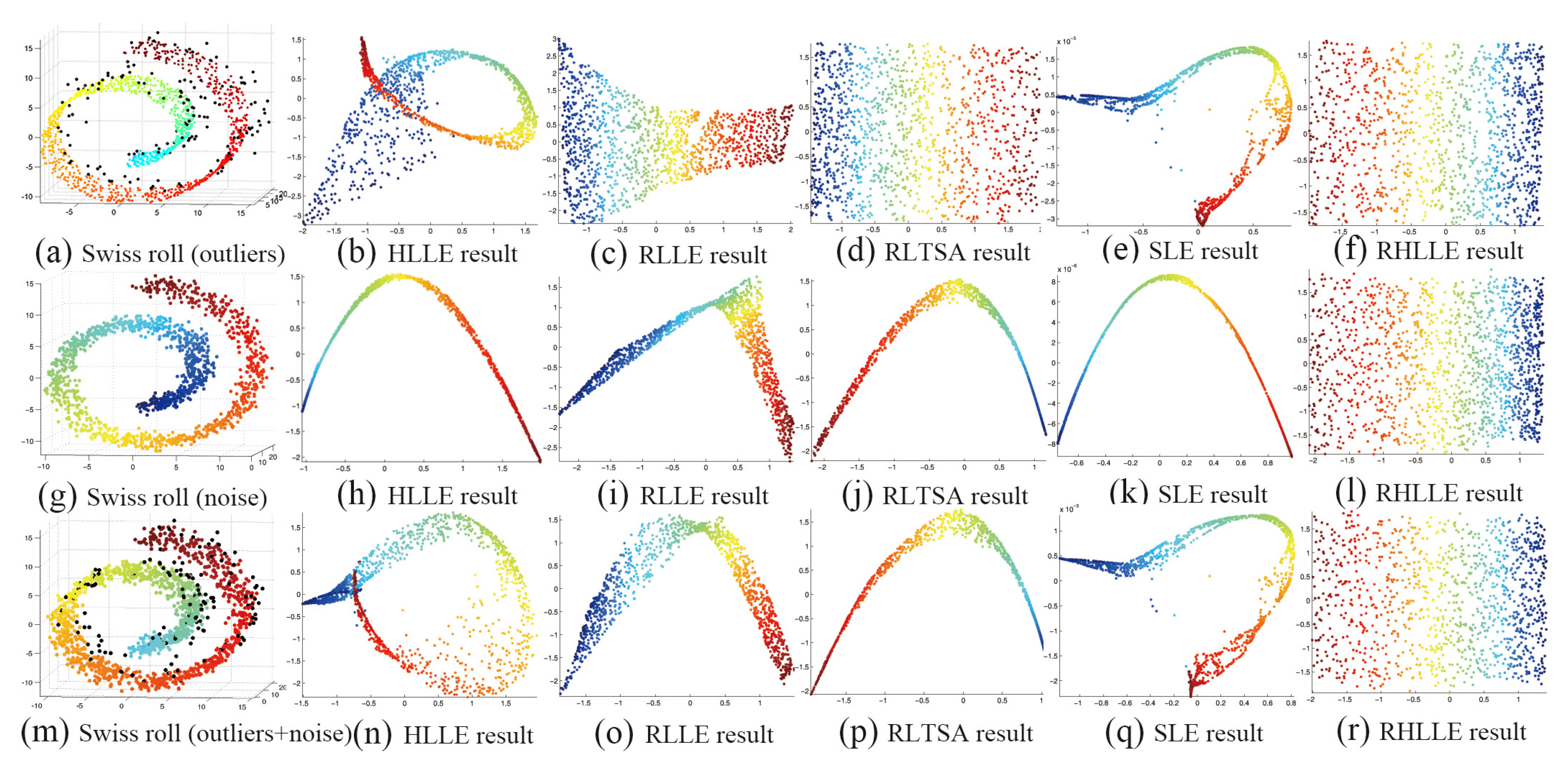
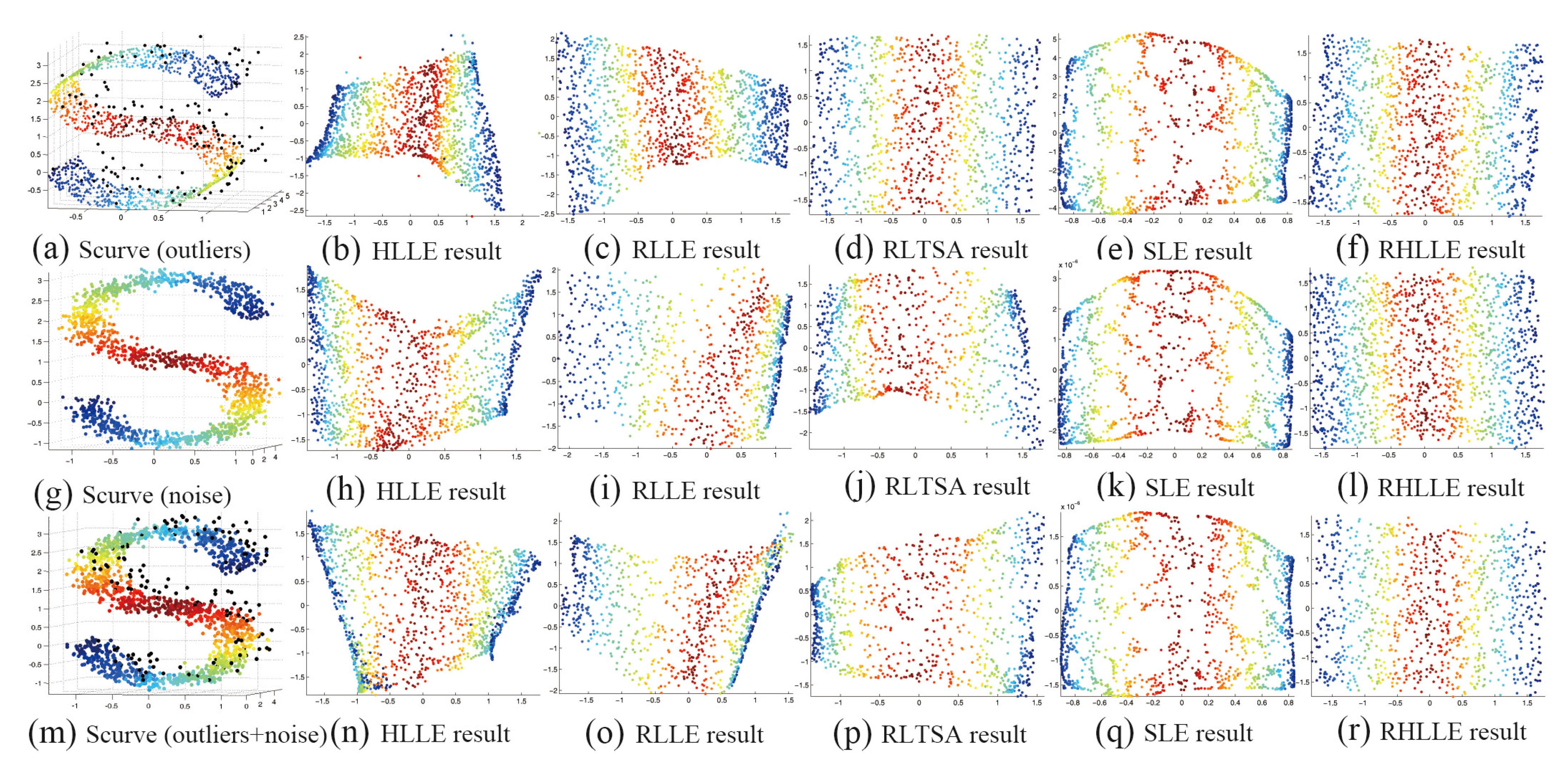
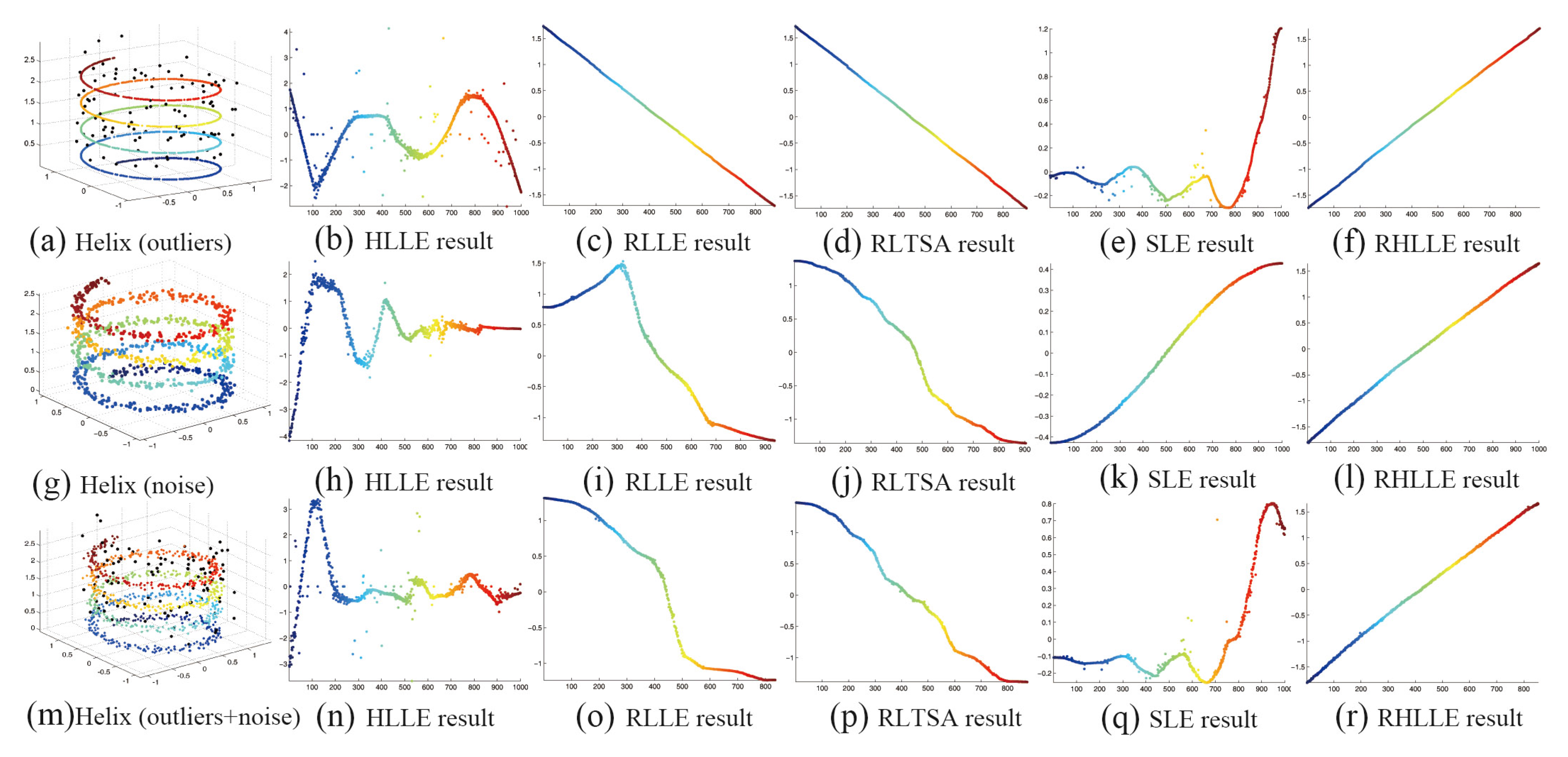
We compare our RHLLE with HLLE [5], RLLE [15], RLTSA [17] and SLE [35] on these datasets. The performance of these algorithms can be seen by comparing the coloring of the data points, the smoothness and the shape of the projection coordinates with their original manifolds. As we can see from Figure 3, Figure 4 and Figure 5, the traditional HLLE algorithm fails to recover the underlying manifold structure when there exist either or both outliers and noise-corrupted points (see Figure 3(b,h and n), Figure 4(b,h and n) and Figure 5(b,h and n). RLLE and RLTSA can recover the manifold structure when there are outliers (see Figure 3(c,d), Figure 4(c,d) and Figure 5(c,d)). However, RLLE and RLTSA cannot recover the manifold structure well when there exist large amounts of noise-corrupted points or both outliers and noise-corrupted points (see Figure 3(i,j,o and p), Figure 4(i,j,o and p) and Figure 5(i,j,o and p)). SLE can usually preserve the local geometry of the data manifolds in the embedding space when there exist large amounts of noise-corrupted points (see Figure 3k, Figure 4k and Figure 5k)). However, SLE cannot preserve the local geometry of the data manifolds well in the embedding space when there exist outliers or both outliers and noise-corrupted points (see Figure 3(e,q), Figure 4(e,q) and Figure 5(e,q)). The results in Figure 3, Figure 4 and Figure 5 show that only our RHLLE algorithm can accurately unfold and recover the original manifolds in the presence of either or both outliers and noise-corrupted points (see Figure 3(f,l and r), Figure 4(f,l and r) and Figure 5(f,l and r)). From the above experiments we can conclude that: (1) our RHLLE algorithm can significantly improve the performance of the Hessian LLE algorithm on the outliers and noise-corrupted data; (2) our RHLLE algorithm performs the best among the five methods on the synthetic datasets.

5.2. High-Dimensional Image Datasets

In the section, we present two experiments on high-dimensional real datasets to illustrate the effectiveness of our RHLLE algorithm. We compare our RHLLE with RLLE, RLTSA and SLE on these datasets.

The first experiment is performed on the teapot image [6] dataset. There are 400 color images of a teapot in this database. They are captured from different angles in a plane. In our experiment, we convert the color images to the 76 × 101 gray-level images, so the dimensionality of the vectorized image space is 7676.

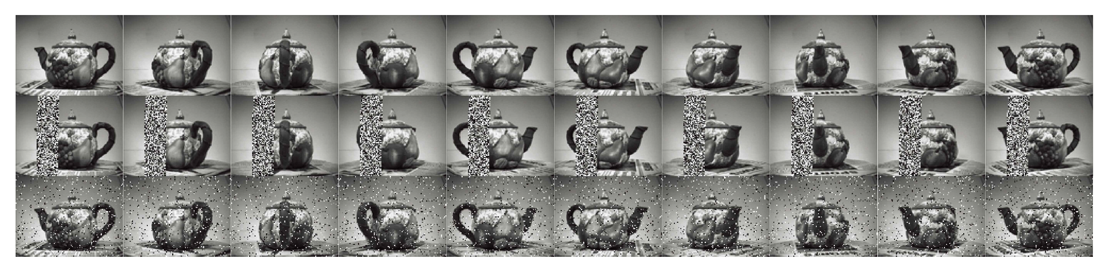
In order to add some outliers to the original image dataset, we first randomly select $10\%$ of the images and for each selected image we replace a rectangular block of the image (about $20\%$ pixels) with independent and identically-distributed samples from a uniform distribution. The location of the corrupt rectangular block is unknown to the algorithm. In order to generate noise-corrupted images, we first randomly select $90\%$ of the images and for each selected image we corrupt $10\%$ of randomly-chosen pixels by replacing their values with independent and identically-distributed samples from a uniform distribution. The corrupted pixels are randomly-chosen for each image, and the locations are unknown to the algorithm. Figure 6 shows 10 original teapot images, their corresponding outlier images and noise-corrupted images.

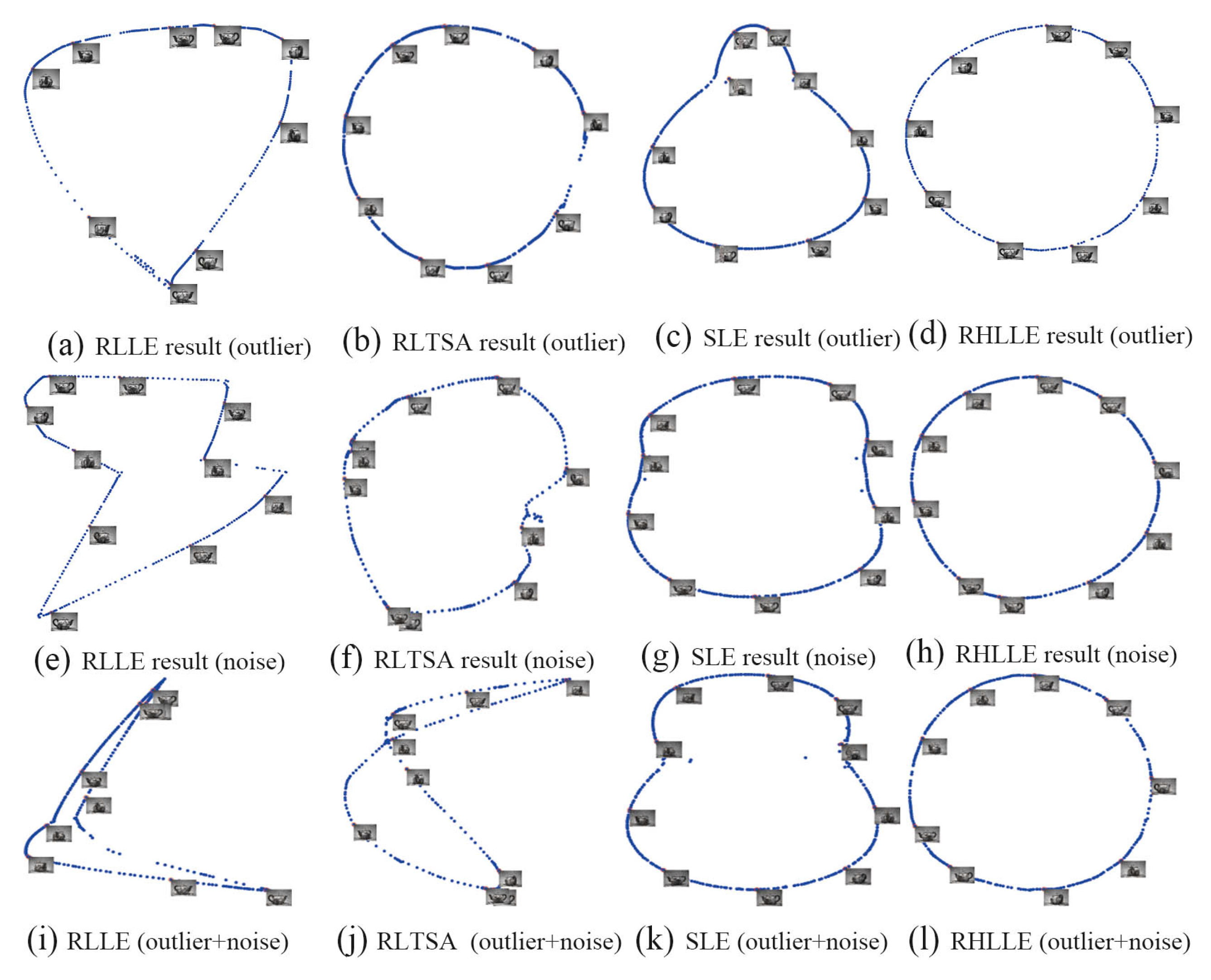
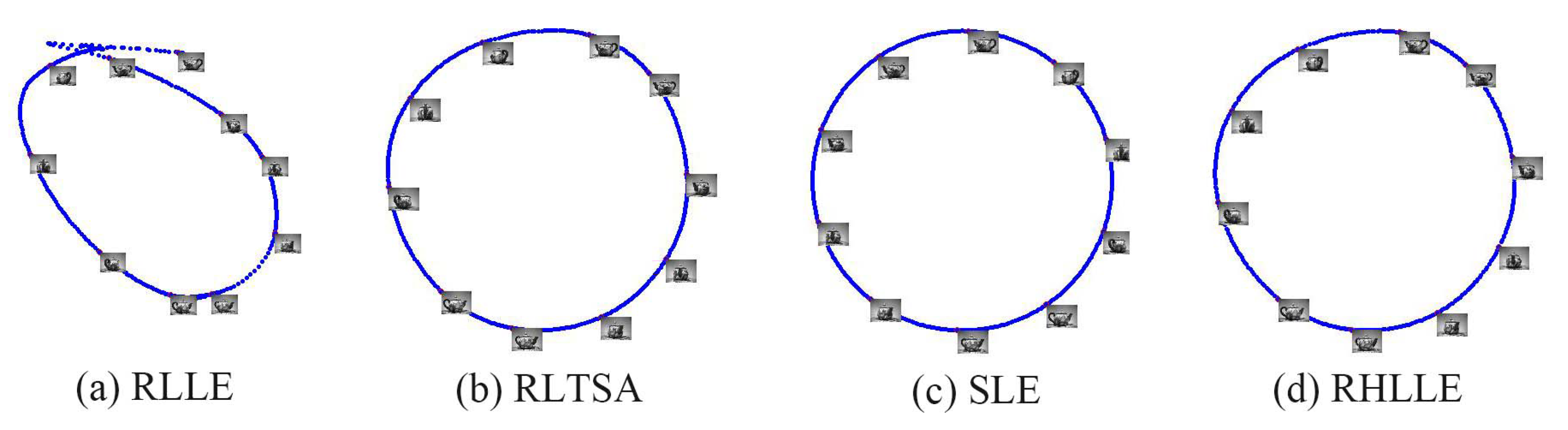
The low-dimensional embeddings in ${\mathbb{R}}^2$ of RLLE, RLTSA, SLE and RHLLE are shown in Figure 7. For completeness and to provide a baseline, the results on the original data without being corrupted are shown in Figure 8. In the embeddings we uniformly mark about $2.5\%$ of the points with red circles and attach their corresponding training images. In the experiment, we set the number of nearest neighbors k to 10. Figure 7 reveals the following points: (1) RLTSA and RHLLE perform better than RLLE and SLE when there are outliers in the image set (see Figure 7a–d); (2) SLE and RHLLE perform better than RLLE and RLTSA when there exist large amounts of noise-corrupted images (see Figure 7e–h); (3) RLLE and RLTSA perform even worse and fail to recover the underlying manifold structure when there exist both outliers and large amounts of noise-corrupted images in the teapot dataset (see Figure 7i,j); (4) The 2D embedding results obtained by our RHLLE are shown in Figure 7d,h and l. Along the circle we can see a clear and smooth change in the orientations of the teapot, which means that our RHLLE successfully uncovers the geometric structure of the image dataset. Therefore, our RHLLE is superior to RLLE, RLTSA and SLE in revealing the underlying manifold when there are either or both outliers and noise-corrupted images in the teapot dataset.

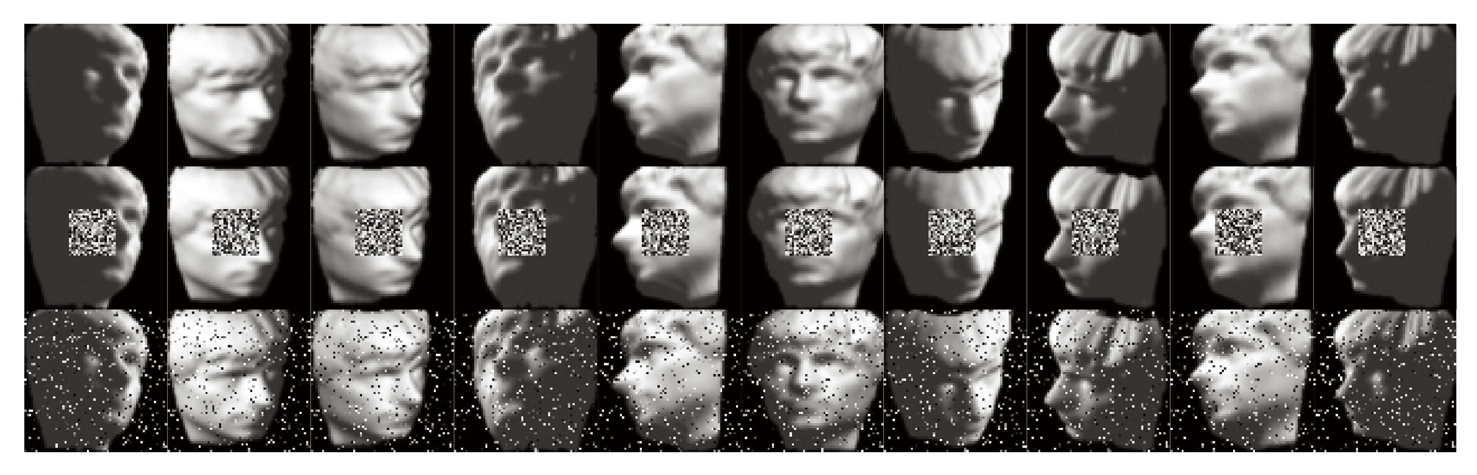
Besides the teapot image dataset, we also conduct experiments on the ISOFACE [1] dataset which is another benchmark dataset used by many manifold learning algorithms. This dataset contains 698 images of a 3D human head, which are collected under different poses and lighting directions. The resolution of each image is 64 × 64 and each image is represented as a 4096-dimensional vector. The intrinsic degrees of freedom are the horizontal rotation, vertical rotation and lighting direction. In order to add some outliers to the original face images, we first randomly select $10\%$ of the images and for each selected face image we replace a square block of the image (about 20% pixels) with independent and identically-distributed samples from a uniform distribution. The location of the corrupt square block is unknown to the computer. In order to generate noise-corrupted face images, we first randomly select $30\%$ of the face images and for each selected image we corrupt $10\%$ of randomly-chosen pixels by replacing their values with independent and identically-distributed samples from a uniform distribution. The corrupted pixels are randomly-chosen for each face image, and the locations are unknown to the algorithm. Figure 9 shows 10 original face images, their corresponding outlier images and noise-corrupted images.

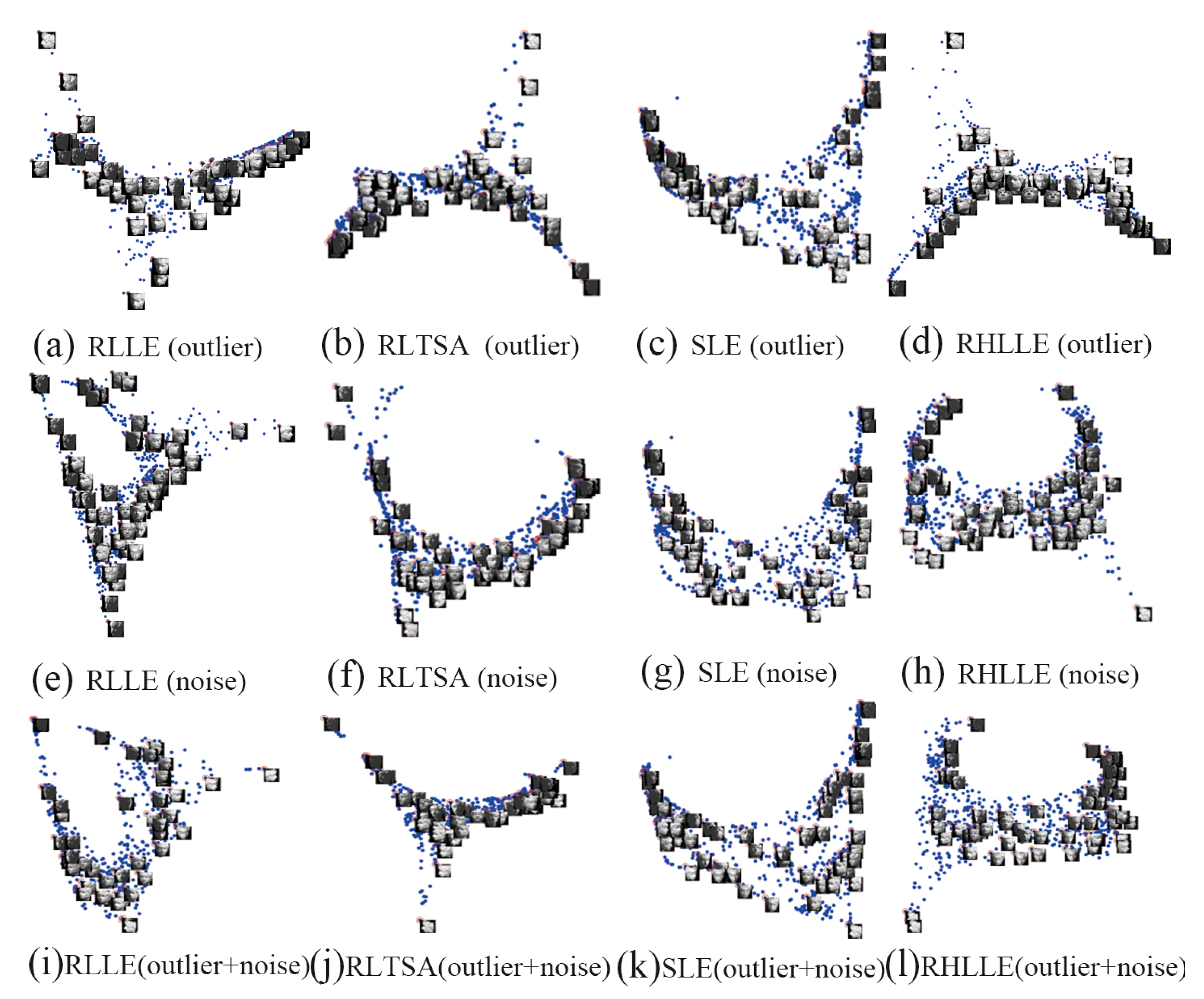
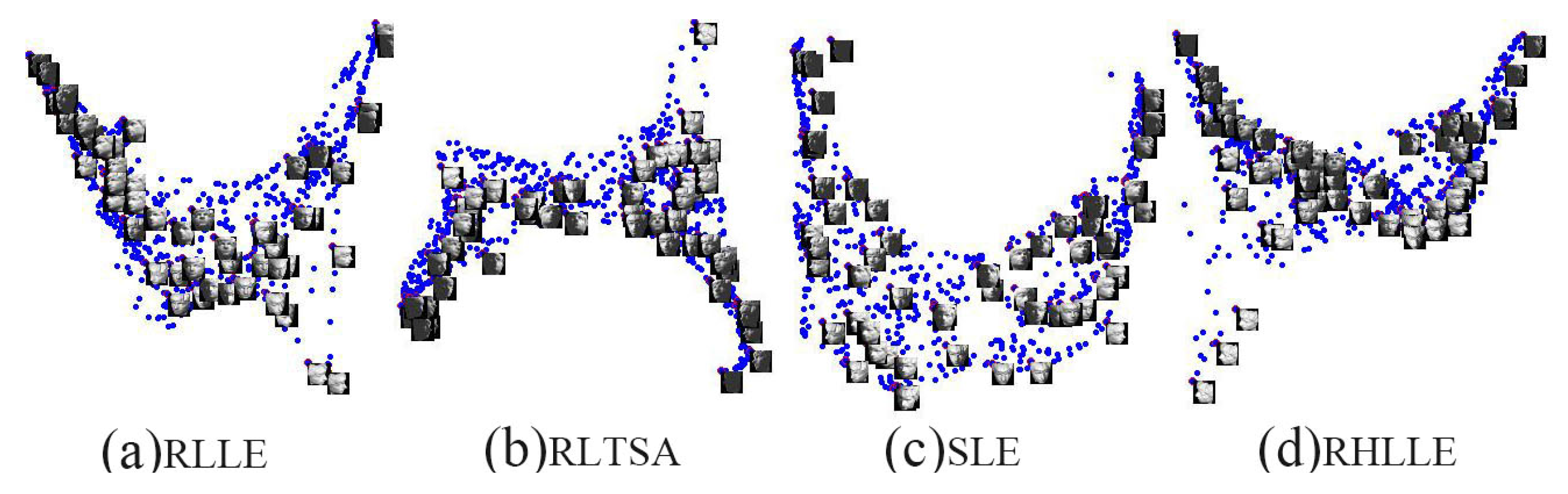
The 2D embedding results of RLLE, RLTSA, SLE and RHLLE are shown in Figure 10. For completeness and to provide a baseline, the results on the original data without being corrupted are shown in Figure 11. In the embedding we randomly mark about $8\%$ points with red circles and attach their corresponding training images. In the experiment, we set the number of nearest neighbors k to 15. Figure 10 reveals several interesting observations: (1) For the outliers situation, the embedding result of RLLE and SLE show that the orientations of the face change smoothly along the horizontal direction and the orientations of the face change from down to up along the vertical direction (see Figure 10a,c). The 2-D embedding results of RLTSA and RHLLE show that the poses and the light of the face images vary smoothly along the horizontal direction and the vertical direction respectively (see Figure 10b,d). Thus, all methods can approximately discover the intrinsic structures of this dataset with outliers; (2) For the noise-corrupted situation, the embedding results of RLLE and RLTSA are severely compressed and the changes in face rotation are not obvious (see Figure 10e and the right-hand side of Figure 10f). Therefore, RLLE and RLTSA cannot recover the underlying manifold structure well when there exist large amounts of noise-corrupted images; (3) For the outliers plus noise-corrupted situation, RLLE and RLTSA perform even worse (see Figure 10i,j), while SLE and our RHLLE successfully reveal the underlying manifold of the ISOFACE dataset with both outliers and noise-corrupted images (see Figure 10k,l).

To further quantitatively evaluate the embedding qualities obtained by RLLE, RLTSA, SLE and our RHLLE, we employ the global smoothness and co-directional consistence (GSCD) criteria introduced in [36]. Roughly speaking, the smaller the value of GSCD, the higher the global smoothness and the better co-directional consistence. For details about the GSCD criteria, please refer to [36].

Table 2. The GSCD results of RLLE, RLTSA, SLE and our RHLLE on the ISOFACE image set with outliers, noise and both outliers and noise respectively.

Method	RLLE	RLTSA	SLE	Our RHLLE
Outlier	0.2865	0.2411	0.2332	0.2294
Noise	0.3322	0.2771	0.1942	0.1843
Outlier+Noise	0.3747	0.3020	0.2148	0.2036

shows the GSCD values computed by different algorithms on the ISOFACE image set with outliers, noise and both outliers and noise respectively. As we can observe from Table 2, our RHLLE algorithm obtains the smallest GSCD value, this result reveals that our RHLLE performs the best in recovering the underlying manifold structure of the ISOFACE dataset with either or both outliers and noise-corrupted points. Moreover, these GSCD results further verify the visualization results (as shown in Figure 10) in a quantitative way.

The average computation times over 10 independent runs of different methods are shown in

Table 3. The average computation time (in seconds) for different methods on synthetic as well as real-world datasets. D denotes the dimensionality of the ambient space and N denotes the number of the data points in each dataset.

Method∖Data	Swiss Roll	S Curve	Helix	Teapot	Isoface
	$\mathit{D}\mathbf{=}\mathbf{3}\mathbf{,}\mathit{N}\mathbf{=}\mathbf{1500}$	$\mathit{D}\mathbf{=}\mathbf{3}\mathbf{,}\mathit{N}\mathbf{=}\mathbf{1500}$	$\mathit{D}\mathbf{=}\mathbf{3}\mathbf{,}\mathit{N}\mathbf{=}\mathbf{1000}$	$\mathit{D}\mathbf{=}\mathbf{7676}\mathbf{,}\mathit{N}\mathbf{=}\mathbf{400}$	$\mathit{D}\mathbf{=}\mathbf{4096}\mathbf{,}\mathit{N}\mathbf{=}\mathbf{698}$
RLLE	1.378	0.976	0.421	1999.3	1248.7
RLTSA	1.482	1.081	0.511	2006.1	1253.9
SLE	463.2	477.8	218.5	10.83	42.65
our RHLLE	1.572	1.256	0.792	514.8	263.3

. As we can observe from Table 3, our RHLLE takes significantly less time than RLLE and RLTSA for high-dimensional datasets. This result is because, for high-dimensional data, the computational complexity of RLLE and RLTSA are dominated by the iterative weighted PCA procedure which has the computational complexity of $O(kNLd{D}^2)$, where L is the number of iterations (usually less than 15); while our RHLLE designs a fast iterative algorithm with low computational complexity $O(kNLD)$ to approximate the original RPCA and the time-consuming reconstruction-errors procedure only need to be computed in one iteration, as we have discussed in Section 4.2. As we can observe from Table 3, SLE takes much more time than other algorithms when the number of data points N is relatively large. This is because that the computational complexity of SLE is dominated by the semi-definite program which scales as $O(N^3+c^3)$, where c is the number of constraints. There are $O(N{k}^2)$ constraints on $O(N^2)$ matrix elements, where k is the number of nearest neighbors [6,35]. Therefore, SLE is more suited for small-scale problems compared to other methods.

6. Conclusions

In this paper, we propose the RHLLE (Robust Hessian LLE) method for robust manifold learning. We introduce a fast algorithm based on robust statistics to identify outliers in high-dimensional data. Moreover, RHLLE uses the local linear smoothing method to reduce the influence of noise. To further reduce the influence of outliers and noise, we propose to incorporate the total reliability scores of reliable local patches as weights into the global functional, then minimize the weighted global functional to obtain robust embedding results. The methods we developed can be used by other manifold learning algorithms to obtain a more accurate reconstruction of the underlying nonlinear manifolds. Extensive experiments on both artificial datasets and real datasets demonstrate the effectiveness of our RHLLE algorithm.

References

- Tenenbaum, J.B.; de Silva, V.; Langford, J.C. A global geometric framework for nonlinear dimensionality reduction. Science 2000, 290, 2319–2323. [Google Scholar] [CrossRef] [PubMed]
- Roweis, S.T.; Saul, L.K. Nonlinear dimensionality reduction by locally linear embedding. Science 2000, 290, 2323–2326. [Google Scholar] [CrossRef] [PubMed]
- Belkin, M.; Niyogi, P. Laplacian eigenmaps and spectral techniques for embedding and clustering. In Advances in Neural Information Processing Systems 14 (NIPS); Dietterich, T.G., Becker, S., Ghahramani, Z., Eds.; Neural information processing systems foundation: Vancouver, BC, Canada, 2001; Volume 14, pp. 585–591. [Google Scholar]
- Zhang, Z.Y.; Zha, H.Y. Principal manifolds and nonlinear dimensionality reduction via tangent space alignment. J. Shanghai Univ. (Engl. Ed.) 2004, 8, 406–424. [Google Scholar] [CrossRef]
- Donoho, D.L.; Grimes, C. Hessian eigenmaps: Locally linear embedding techniques for high-dimensional data. Proc. Natl. Acad. Sci. 2003, 100, 5591–5596. [Google Scholar] [CrossRef] [PubMed]
- Weinberger, K.Q.; Saul, L.K. Unsupervised learning of image manifolds by semidefinite programming. Int. J. Comput. Vis. 2006, 70, 77–90. [Google Scholar] [CrossRef]
- Lin, T.; Zha, H. Riemannian manifold learning. IEEE Trans. Pattern Anal. Mach. Intell. 2008, 30, 796–809. [Google Scholar] [PubMed]
- Wang, R.; Shan, S.; Chen, X.; Chen, J.; Gao, W. Maximal linear embedding for dimensionality reduction. IEEE Trans. Pattern Anal. Mach. Intell. 2011, 33, 1776–1792. [Google Scholar] [CrossRef] [PubMed]
- Xing, X.; Wang, K.; Lv, Z.; Zhou, Y.; Du, S. Fusion of Local Manifold Learning Methods. IEEE Signal Process. Lett. 2015, 22, 395–399. [Google Scholar] [CrossRef]
- Seung, H.S.; Lee, D.D. The manifold ways of perception. Science 2000, 290, 2268–2269. [Google Scholar] [CrossRef] [PubMed]
- Belkin, M.; Niyogi, P.; Sindhwani, V. Manifold regularization: A geometric framework for learning from labeled and unlabeled examples. J. Mach. Learn. Res. 2006, 7, 2399–2434. [Google Scholar]
- Xing, X.; Yu, Y.; Jiang, H.; Du, S. A multi-manifold semi-supervised Gaussian mixture model for pattern classification. Pattern Recognit. Lett. 2013, 34, 2118–2125. [Google Scholar] [CrossRef]
- Souvenir, R.; Pless, R. Manifold clustering. In Proceeding of the Tenth IEEE International Conference on Computer Vision, ICCV 2005, Beijing, China, 17–21 October 2005; Volume 1, pp. 648–653.
- Hawkins, D.M. Identification of Outliers; Springer: New York, NY, USA, 1980; Chapter 1. [Google Scholar]
- Chang, H.; Yeung, D.Y. Robust locally linear embedding. Pattern Recognit. 2006, 39, 1053–1065. [Google Scholar] [CrossRef]
- De La Torre, F.; Black, M.J. A framework for robust subspace learning. Int. J. Comput. Vis. 2003, 54, 117–142. [Google Scholar] [CrossRef]
- Zhan, Y.; Yin, J. Robust local tangent space alignment via iterative weighted PCA. Neurocomputing 2011, 74, 1985–1993. [Google Scholar] [CrossRef]
- Zhang, Z.; Zha, H. Local Linear Smoothing for Nonlinear Manifold Learning; Technical Report; CSE, Penn State University: Old Main, PA, USA, 2003. [Google Scholar]
- Park, J.; Zhang, Z.; Zha, H.; Kasturi, R. Local smoothing for manifold learning. In Proceedings of the 2004 IEEE Computer Society Conference on Computer Vision and Pattern Recognition, Washington, DC, USA, 27 June–2 July 2004; Volume 2, pp. 445–452.
- Hein, M.; Maier, M. Manifold denoising. In Advances in Neural Information Processing Systems 19 (NIPS); Schölkopf, B., Platt, J.C., Hoffman, T., Eds.; Neural Information Processing System Foundation: Vancouver, BC, Canada, 2006; Volume 19, pp. 561–568. [Google Scholar]
- Zhou, D.; Bousquet, O.; Lal, T.N.; Weston, J.; Schölkopf, B. Learning with Local and Global Consistency. In Advances in Neural Information Processing Systems 16 (NIPS); Thrun, S., Saul, L.K., Schölkopf, B., Eds.; Neural Information Processing Systems Foundation: Vancouver, BC, Canada, 2003; Volume 16, pp. 321–328. [Google Scholar]
- Xing, X.; Du, S.; Jiang, H. Semi-Supervised Nonparametric Discriminant Analysis. IEICE Trans. Inf. Syst. 2013, 96, 375–378. [Google Scholar] [CrossRef]
- Gashler, M.; Martinez, T. Robust manifold learning with CycleCut. Connect. Sci. 2012, 24, 57–69. [Google Scholar] [CrossRef]
- Chern, S.S.; Chen, W.H.; Lam, K.S. Lectures on Differential Geometry; World Scientific Pub Co Inc.: Singapore, 1999; Volume 1. [Google Scholar]
- Huber, P.J. Robust Statistics; Springer: Berlin, Germany, 2011. [Google Scholar]
- Kim, K.I.; Steinke, F.; Hein, M. Semi-Supervised Regression Using Hessian Energy with an Application to Semi-Supervised Dimensionality Reduction. In Advances in Neural Information Processing Systems 22 (NIPS); Bengio, Y., Schuurmans, D., Lafferty, J.D., Williams, C.K.I., Culotta, A., Eds.; Neural Information Processing Systems Foundation: Vancouver, BC, Canada, 2009; Volume 22, pp. 979–987. [Google Scholar]
- Lin, B.; He, X.; Zhang, C.; Ji, M. Parallel vector field embedding. J. Mach. Learn. Res. 2013, 14, 2945–2977. [Google Scholar]
- Lin, B.; Zhang, C.; He, X. Semi-Supervised Regression via Parallel Field Regularization. In Advances in Neural Information Processing Systems 24 (NIPS); Shawe-Taylor, J., Zemel, R.S., Bartlett, P.L., Pereira, F., Weinberger, K.Q., Eds.; Neural Information Processing Systems Foundation: Granada, Spain, 2011; Volume 24. [Google Scholar]
- Turk, M.; Pentland, A. Eigenfaces for recognition. J. Cognit. Neurosci. 1991, 3, 71–86. [Google Scholar] [CrossRef] [PubMed]
- Zhang, P.; Qiao, H.; Zhang, B. An improved local tangent space alignment method for manifold learning. Pattern Recognit. Lett. 2011, 32, 181–189. [Google Scholar] [CrossRef]
- De la Torre, F.; Black, M.J. Robust principal component analysis for computer vision. In Proceeding of the Eighth IEEE International Conference on Computer Vision, 2001. ICCV 2001, Vancouver, BC, USA; 2001; Volume 1, pp. 362–369. [Google Scholar]
- Holland, P.W.; Welsch, R.E. Robust regression using iteratively reweighted least-squares. Commun. Stat. Theory Methods 1977, 6, 813–827. [Google Scholar] [CrossRef]
- Huber, P.J. Robust regression: Asymptotics, conjectures and Monte Carlo. Ann. Stat. 1973, 1, 799–821. [Google Scholar] [CrossRef]
- Cleveland, W.S.; Loader, C. Smoothing by Local Regression: Principles and Methods. In Statistical Theory and Computational Aspects of Smoothing; Springer: Heidelberg, Germany, 1996; pp. 10–49. [Google Scholar]
- Hou, C.; Zhang, C.; Wu, Y.; Jiao, Y. Stable local dimensionality reduction approaches. Pattern Recognit. 2009, 42, 2054–2066. [Google Scholar] [CrossRef]
- Zhang, J.; Wang, Q.; He, L.; Zhou, Z.H. Quantitative analysis of nonlinear embedding. IEEE Trans. Neural Netw. 2011, 22, 1987–1998. [Google Scholar] [CrossRef] [PubMed]
Figure 1.
Embeddings of the synthetic 2D manifolds. (a) Swiss Roll with a hole; (b) S-curve; (c) Uniform Swiss Roll; (d) Punched Sphere. The first row shows the four manifolds, and the second (e–h) and third rows; (i–l) are the corresponding embedding results obtained by the original HLLE and our reformulated HLLE respectively. In all experiments, the number of data samples is 1000 and the number of nearest neighbors is fixed to .
Figure 2.
Results of HLLE, RLLE and RHLLE applied to the “Swiss roll with a hole” dataset with the existence of outliers and noises. (a) Dataset with outliers and noises; (b) Results of outlier removal using RLLE’s method; (c) Results of outlier removal using RHLLE’s method; (d) Cumulative distributions of reliability scores computed by the RLLE’s method; (e) Cumulative distributions of reliability scores computed by the RHLLE’s method; (f) Results of noise reduction with one iteration of local smoothing; (g) HLLE result; (h) RLLE result; (i) RHLLE result.
Figure 3.
The first row shows the Swiss roll dataset with outliers and the embedding results of different algorithms;The second row shows the Swiss roll dataset with noise and the embedding results of different algorithms; The third row shows the Swiss roll dataset with both outliers and noise and the embedding results of different algorithms.
Figure 4.
The first row shows the S-curve dataset with outliers and the embedding results of different algorithms; The second row shows the S-curve dataset with noise and the embedding results of different algorithms; The third row shows the S-curve dataset with both outliers and noise and the embedding results of different algorithms.
Figure 5.
The first row shows the Helix curve dataset with outliers and the embedding results of different algorithms; The second row shows the Helix curve dataset with noise and the embedding results of different algorithms; The third row shows the Helix curve dataset with both outliers and noise and the embedding results of different algorithms.
Figure 6.
Ten teapot images, their corresponding outlier images and noise-corrupted images.
Figure 7.
2D embedding results of RLLE, RLTSA, SLE and RHLLE on the teapot image set with outliers, noise and both outliers and noise respectively.
Figure 8.
2D embedding results of RLLE, RLTSA, SLE and RHLLE on the original teapot image set without being corrupted.
Figure 9.
Ten ISOFACE images, their corresponding outlier images and noise-corrupt images.
Figure 10.
2-D embedding results of RLLE, RLTSA, SLE and RHLLE on the ISOFACE image set with outliers, noise and both outliers and noise respectively.
Figure 11.
2D embedding results of RLLE, RLTSA, SLE and RHLLE on the original ISOFACE image set without being corrupted.