Article

The Parameterized Complexity of the Rainbow Subgraph Problem †

Institut für Softwaretechnik und Theoretische Informatik, TU Berlin, Ernst-Reuter-Platz 7, D-10587 Berlin, Germany
*
Author to whom correspondence should be addressed.
This paper is an extended version of our paper published in the Proceedings of the 40th International Workshop on Graph-Theoretic Concepts in Computer Science (WG 2014), Nouan-le-Fuzelier, France, 25–27 June 2014.
Algorithms 2015, 8(1), 60-81; https://doi.org/10.3390/a8010060
Submission received: 22 September 2014 / Revised: 13 February 2015 / Accepted: 16 February 2015 / Published: 27 February 2015

Abstract

:
The NP-hard RAINBOW SUBGRAPH problem, motivated from bioinformatics, is to find in an edge-colored graph a subgraph that contains each edge color exactly once and has at most k vertices. We examine the parameterized complexity of RAINBOW SUBGRAPH for paths, trees, and general graphs. We show that RAINBOW SUBGRAPH is W[1]-hard with respect to the parameter k and also with respect to the dual parameter := nk where n is the number of vertices. Hence, we examine parameter combinations and show, for example, a polynomial-size problem kernel for the combined parameter and “maximum number of colors incident with any vertex”. Additionally, we show APX-hardness even if the input graph is a properly edge-colored path in which every color occurs at most twice.

1. Introduction

The RAINBOW SUBGRAPH problem is defined as follows.
RAINBOW SUBGRAPH
Instance: An undirected graph G = (V, E), an edge coloring χ : E → {1, …, p} for some p ≥ 1, and an integer k ≥ 0.
Question: Is there a subgraph G′ of G that contains each edge color exactly once and has at most k vertices?
We call a subgraph G′ with these properties a solution of order at most k. In the problem name, the term rainbow refers to the fact that all edges of G″ have a different color. For convenience, we define a rainbow cover as a subgraph where every color occurs at least once; these definitions are illustrated in Figure 1. Note that every rainbow cover G′ of order at most k has a subgraph that is a solution: Simply remove any edge whose color appears more than once in G′. Repeating this operation as long as possible yields a solution of the same order as G′.
RAINBOW SUBGRAPH arises in bioinformatics: there is a natural reduction from the (POPULATION) PARSIMONY HAPLOTYPING problem to RAINBOW SUBGRAPH [1,2]. In PARSIMONY HAPLOTYPING, one aims to reconstruct a set of chromosome types, called haplotypes, from an observed set of genotypes. Each genotype consists of exactly two haplotypes; these haplotypes explain the observed genotype. There can be, however, more than one possibility of explaining a genotype by two haplotypes. In the reduction to RAINBOW SUBGRAPH, the approach is to first compute all possible explanations for each genotype. Then, each haplotype that occurs in at least one possible explanation becomes a vertex of the graph. Each pair of haplotypes that explains one of the input genotypes is connected by an edge, and this edge receives the label of the genotype as edge color. Selecting a minimum number of haplotypes that explains all genotypes is now equivalent to finding a minimum-size vertex set that induces a graph containing all edge colors. Note that in the worst case, this reduction might not produce a polynomial-size instance, as the number of possible explanations of each genotype may become exponential. Another bioinformatics application appears in the context of PCR primer set design [1,3].

1.1. Related Work

The optimization version of RAINBOW SUBGRAPH has been mostly studied in terms of polynomial-time approximability. Here the optimization goal is to minimize the number of vertices in the solution; we refer to this problem as MINIMUM RAINBOW SUBGRAPH. MINIMUM RAINBOW SUBGRAPH is APX-hard even on graphs with maximum vertex degree Δ ≥ 2 in which every color occurs at most twice [4]. Moreover, MINIMUM RAINBOW SUBGRAPH cannot be approximated within a factor of c ln Δ for some constant c unless NP has slightly superpolynomial time algorithms [5].
The more general MINIMUM-WEIGHT MULTICOLORED SUBGRAPH problem, where each vertex has a nonnegative weight and we minimize the total weight of the vertices chosen, has a randomized q log p-approximation algorithm, where q is the maximum number of times any color occurs in the input graph [1]. MINIMUM RAINBOW SUBGRAPH can be approximated within a ratio of (δ + ln[δ] + 1)/2, where δ is the average vertex degree in the solution [6]. Katrenič and Schiermeyer [4] presented an exact algorithm for RAINBOW SUBGRAPH that has running time 2p ·Δ2p ·nO(1), where n is the order of the input graph and Δ is the maximum vertex degree of the input graph. This is the only previous fixed-parameter algorithm for MINIMUM RAINBOW SUBGRAPH that we are aware of. There are, however, several results on the parameterized complexity of PARSIMONY HAPLOTYPING [79]. RAINBOW SUBGRAPH is also a special case of SET COVER WITH PAIRS [10] which, in graph-theoretic terms, corresponds to the case where the input is a multigraph with vertex weights and the aim is to find a minimum-cost rainbow cover.

1.2. Our Contributions

Since RAINBOW SUBGRAPH is NP-hard even on collections of paths and cycles [4], we perform a broad parameterized complexity analysis. Table 1 gives an overview of the complexity of MINIMUM RAINBOW SUBGRAPH on paths, trees, and general graphs, when parameterized by
  • p: number of colors;
  • k: number of vertices in the solution;
  • := nk: number of vertex deletions to obtain a solution;
  • Δ: maximum vertex degree;
  • ΔC := maxυ∈V |{c | ∃{u, υ} ∈ E : χ({u, υ}) = c}|: maximum color degree;
  • q: maximum number of times any color occurs in the input graph.
For each parameter and some parameter combinations, we give either a fixed-parameter algorithm or show W[1]-hardness. Our main results are as follows: RAINBOW SUBGRAPH is APX-hard even if the input graph is a properly edge-colored path with q = 2; this strengthens a previous hardness result [4]. RAINBOW SUBGRAPH is W[1]-hard on general graphs for each of the considered parameters; this rules out fixed-parameter algorithms for most natural parameters. For the number of colors p, solution order k, and number of vertex deletions, the complexity seems to depend on the density of the graph as the problem is W[1]-hard for each of these parameters but it becomes tractable if any of these parameters is combined with the maximum degree Δ. Our algorithm for the parameter combination (Δ, p) improves a previous algorithm for the same parameters [4]. For trees, we show a difference between the parameters p and : in this case, RAINBOW SUBGRAPH is fixed-parameter tractable for the parameters k or p, but W[1]-hard for the parameter .

2. Preliminaries

We use n and m to denote the number of vertices and edges in the input graph, respectively. The order of a graph G is the number n of vertices in G. We call a graph G′ = (V, E′) induced subgraph of a graph G = (V, E) if V′ ⊆ V and E′ = {{u, υ } | u, υV′ and {u, υ} ∈ E}. The graph induced by a vertex set V′ in G is denoted G[V′]. The degree of a vertex υ is denoted deg(υ).
APX is the class of optimization problems that allow polynomial-time approximation algorithms with a constant approximation factor. If a problem is APX-hard, then it cannot be approximated in polynomial time to arbitrary constant factors, unless P = NP. To show that a problem is APX-hard, we can use an L-reduction from a known APX-hard problem. An L-reduction from a problem Π to a problem Π′ produces from an instance I of Π in polynomial time an instance I′ of Π′ such that for some constant a, OPT(I′) < a · OPT(I); additionally, it must be possible in polynomial time to produce from a feasible solution of I′ of value x′ a feasible solution of I of value x where | OPT(I) − x| ≤ b| OPT(I′) − x′| for some constant b ([11], Definition 16.4).
An instance of a parameterized problem is a pair (I, x), where x is some problem-specific parameter, typically a nonnegative integer [1214]. A problem is called fixed-parameter tractable (FPT) with respect to x if it can be solved in f(x) · |I|O(1) time, where f is an arbitrary computable function. A data reduction (rule) is a polynomial-time self-reduction for a parameterized problem, that is, it replaces in polynomial time an instance (I, x) with an instance (I′, x′) such that I′ has a solution with respect to the new parameter x′ if and only if I has a solution with respect to the original parameter x; we say that the rule is correct when this property holds. We say that an instance is reduced with respect to a reduction rule if the rule does not affect the instance. If the size of I′ depends only on some function of x, we say that we have a problem kernel with respect to parameter x.
Analogously to NP, the class W[1] captures parameterized hardness [1214]. It is widely assumed that if a problem is W[1]-hard, then it is not fixed-parameter tractable. One can show W[1]-hardness by a parameterized reduction from a known W[1]-hard problem. This is a reduction that runs in f(x) · |I|O(1) time for some function f and maps the parameter x to a new parameter x′ that is bounded by some function of x.
We will use the following simple observation several times.
Observation 1. Let G′ = (V, E′) be a solution for a RAINBOW SUBGRAPH instance with G = (V, E). If there are two vertices u, υ in Vsuch that {u, υ} ∈ E but {u, υ} ∉ E, then there is a solution Gthat does contain the edge {u, υ} and has the same number of vertices.
Observation 1 is true since replacing the edge in G′ that has the same color as {u, υ} by {u, υ} is a solution.
Next, we list some basic observations regarding parameter bounds and relations between parameters of MINIMUM RAINBOW SUBGRAPH. Let (G, χ) be an instance of MINIMUM RAINBOW SUBGRAPH and let S be a solution to G. Since a graph with n vertices contains at most n(n − 1)/2 edges, we can assume for the order k of a solution and the number p of colors that
p k ( k 1 ) / 2
A graph with n vertices and maximum vertex degree Δ has at most nΔ/2 edges; so if G has maximum vertex degree Δ, then
p k Δ / 2
If the solution S contains no cycles, then p ≤ |V (S)| − 1, so if G is acyclic, then we can assume
p k 1

3. Parameterization by Color Occurrences

We now consider the complexity of RAINBOW SUBGRAPH parameterized by the maximum number q of color occurrences. Indeed, the value of q is bounded in some applications: For example in the graph formulation of PARSIMONY HAPLOTYPING, q depends on the maximum number of ambiguous positions in a genotype, which can be assumed to be small.
Katrenič and Schiermeyer [4] showed that MINIMUM RAINBOW SUBGRAPH is APX-hard for Δ = 2. The instances produced by their reduction contain precisely two edges of each color, so APX-hardness even holds for q = 2. However, the resulting graph contains cycles and is not properly edge-colored, so the complexity on acyclic graphs and on properly edge-colored graphs (like those resulting from PARSIMONY HAPLOTYPING instances) remains to be explored. We show that neither restriction is helpful, as RAINBOW SUBGRAPH is APX-hard for properly edge-colored paths with q = 2. This strengthens the hardness result of Katrenič and Schiermeyer [4]. For this purpose, we develop an L-reduction (see Section 2) from the following special case of MINIMUM VERTEX COVER:
MINIMUM VERTEX COVER IN CUBIC GRAPHS
Instance: An undirected graph H = (W, F) in which every vertex has degree three.
Task: Find a minimum-cardinality vertex cover of G.
MINIMUM VERTEX COVER IN CUBIC GRAPHS is APX-hard [15].
Theorem 1. MINIMUM RAINBOW SUBGRAPH is APX-hard even when the input is a properly edge-colored path in which every color occurs at most twice.
Proof. Given an instance H = (W = {w1, …, wn}, F) of MINIMUM VERTEX COVER IN CUBIC GRAPHS, construct an edge-colored path G = (V, E) as follows. The vertex set is V := {υ1, …, υ16n+2}. The edge set is E := {{υi, υi+1} | 1 ≤ i ≤ 16n + 1}, that is, vertices with successive indices are adjacent. It remains to specify the edge colors. Herein, we use u* to denote unique colors, that is, if an edge is u*-colored, then it receives an edge color that does not appear anywhere else in G. In addition to these unique colors, introduce five colors for each vertex of H, that is, for each wiW create edge colors ci, c i, c i, xi, and yi. The colors ci, c i, and c i are “filling” colors which are needed because G is connected. Furthermore, for each edge fiF introduce a unique edge color ϕi.
Now, color the first 6n + 1 edges of G by the following sequence.
Algorithms 08 00060f3
That is, the edge between υ1 and υ2 is u*-colored, the edge between υ2 and υ3 is c1-colored, and so on. The u*-colors are unique and thus occur only once in G. Consequently, both endpoints of these colors are contained in every solution.
Now for each vertex wi in H color 10 edges in G according to the edges that are incident with wi. More precisely, for each wi color the edges from υ6n+2+10(i−1) to υ6n+2+10i. We call the subpath of G with these vertices the wi-part of G. Let {fr, fs, ft} denote the set of edges incident with wi. Then color the edges between υ6n+2+10(i−1) and υ6n+2+10i by the following sequence.
Algorithms 08 00060f4
The resulting graph is a path with exactly 16n + 1 edges and p = 8n + |F | + 1 colors.
The idea of the construction is that we may use the vertices of the wi-part to “cover” the colors corresponding to the edges incident with wi. If we do so, then the solution has two connected components in the wi-part. Otherwise, it is sufficient to include one connected component from the wi-part. Since the solution graph is acyclic and the number of edges in a minimal solution is fixed, the number of connected components in the solution and its order are equal up to an additive constant.
We now show formally that the reduction fulfills the two properties of L-reductions (see Section 2). Let S* be an optimal vertex cover for the MINIMUM VERTEX COVER IN CUBIC GRAPHS instance and let G* be an optimal solution to the constructed MINIMUM RAINBOW SUBGRAPH instance.
The first property we need to show is that |V (G*)| = O(|S*|). As observed above, the number of colors p in G is O(n + |F |) and thus |V (G*)| 2p = O(n + |F|). Clearly, S* contains at least |F |/3 vertices, since every vertex in H covers at most three edges. Moreover, since H is cubic we have n < 2|F | and thus |S*| = Θ(n + |F |). Consequently, |V (G*)| = O(|S*|).
The second property we need to show is the following: given a solution G′ to G, we can compute in polynomial time a solution S′ to H such that
| S | | S | = O ( | V ( G ) | | V ( G ) | ) .
Let G′ be a solution to G. The proof outline is as follows. We show that G′ has order p+n+1+x, x ≥ 0, and that, given G′, we can compute in polynomial time a size-x vertex cover S′ of H. Then we show that, conversely, there is a solution of order at most p + n + 1 + |S*|. Thus, the differences between the solution sizes in the MINIMUM VERTEX COVER IN CUBIC GRAPHS instance and in the MINIMUM RAINBOW SUBGRAPH instance are essentially the same.
We now show that G′ has order p + n + 1 + x, x ≥ 0. Since G′ is a solution it contains each edge color exactly once. Thus, G′ has exactly p edges. We now apply a series of modifications to G′ that do not increase the order of G′. The aim of these modifications is to put all of the first 6n + 1 edges of G into G′. This can be achieved as follows: If G′ contains an edge with a color ci, c i, or c i such that its endpoints are not among the first 6n + 2 vertices, then remove this edge from G′ and add the uniquely defined edge with the same color whose endpoints are among the first 6n + 2 vertices. As observed above, each of these first vertices is contained in every solution and therefore also in G′. Due to Observation 1, this modification thus does not increase the order of G′ and maintains that G′ is a solution. Hence, we assume from now on that G′ contains all of the first 6n + 1 edges of G and no other edges of color ci, c i, or c i. This implies that each connected component of G′ is either fully contained in the first part or fully contained in some wi-part (since the first edge of each such part has a c-color). Moreover, every wi-part contains at least one connected component of G′, as the colors xi and yi occur only in this part. Therefore, G′ has n + 1 + x components for some x ≥ 0. Since G′ is acyclic, the order of G′ thus is p + n + 1 + x.
Now, construct S′ in polynomial time as follows. Consider each wi-part of G. Let {fr, fs, ft} denote the edges of H that are incident with wi. If one of the connected components of G′ that is contained in the wi-part contains an edge with color ϕr, ϕs, or ϕt, then add wi to S′.
First, we show that |S′| ≤ x. Consider a wi-part of G such that wiS′. By the discussion above, the connected components of G′ that are contained in the wi-part of G do not contain edges with color ci, c i, or c i. Hence, these connected components are subgraphs of the following graph that has three connected components:
Algorithms 08 00060f5
Every subgraph of this graph that contains the edge colors xi, yi, and one of the other three colors ϕr, ϕs, and ϕt has at least two connected components. Hence, for each wiS′, G′ has at least two connected components in the wi-part. Further, for each other wi-part, G′ has at least one connected component. Finally, G′ has one further connected component consisting of the first 6n + 1 edges. Altogether, the number of connected components thus is at least n + 1 + |S′| and thus |S′| ≤ x.
Second, we show that S′ is a vertex cover of H: Since G′ contains an edge of every color, there is for each edge fjF at least one wi-part such that G′ contains an edge with color ϕj from this part. By the construction of S′, we have wiS′. Summarizing, we have shown that if there is a solution G′, then it has p + 1 + n + x vertices for some x ≥ 0 and from such a solution we can construct a vertex cover S′ of size at most x.
Now, let τ := |S′| − |S*|. We show that there is a solution Ĝ to G which needs at most |V (G′)| − τ vertices. Construct Ĝ as follows. For each edge fiF select an arbitrary vertex of S* that is incident with fi. Then, add the edge with color ϕi in the subpath of G that corresponds to wi and its endpoints to Ĝ. For each subpath where at least one edge has been added in this way, add the first x- and y-edge and its endpoints to Ĝ. For all other subpaths, add the second x- and y-edge to Ĝ. Finally, add the first 6n + 1 edges of G plus their endpoints to Ĝ. Then, Ĝ contains p edges, one for each color. The number of connected components in Ĝ is 1 + 2|S*| + n − |S*|, hence, the number of vertices in Ĝ is p + 1 + |S*| + n. Consequently, we have
| V ( G ) | | V ( G ^ ) | = p + 1 + x + n ( p + 1 + | S | + n ) | S | | S | = τ .
Now an optimal solution G* has at most as many vertices as Ĝ, and thus
| V ( G ) | | V ( G ) | | V ( G ) | | V ( G ^ ) | | S | | S | = τ
which directly implies Equation (4). □

4. Parameterization by Number of Colors

We now consider the parameter number of colors p. We show that RAINBOW SUBGRAPH is generally W[1]-hard with respect to p, but becomes fixed-parameter tractable if the input graph is sparse. Recall that we assume Inequality (1) which states that pk(k − 1)/2. Moreover, we can construct a solution by arbitrarily selecting one edge of each color, implying k ≤ 2p in nontrivial instances. Thus, the parameter p is polynomially upper- and lower-bounded by the solution order k. In consequence, while our main focus is on parameter p, every parameterized complexity classification for p also implies the corresponding parameterized complexity classification for k.

4.1. Hardness on Bipartite Graphs

A graph G is called d-degenerate if every subgraph of G has a vertex of degree at most d. We can show that even on 2-degenerate bipartite graphs, the decision problem RAINBOW SUBGRAPH is W[1]-hard for parameter p (and thus also for parameter k) by a parameterized reduction from the MULTICOLORED CLIQUE problem.
Theorem 2. MINIMUM RAINBOW SUBGRAPH is W[1]-hard with respect to the number of colors p, even if the input graph is 2-degenerate and bipartite.
Proof. We give a parameterized reduction from the following well-known problem:
MULTICOLORED CLIQUE
Instance: An undirected graph G = (V, E) with proper vertex coloring χV : V →{1, …, pV}.
Question: Does G have a clique of order pV?
Here, proper means that {u, υ} ∈ EχV (u) ≠ χV (υ). MULTICOLORED CLIQUE is W[1]-complete with respect to parameter pV [16].
Let (G = (V, E), χV) be an instance of MULTICOLORED CLIQUE. We construct a bipartite edge-colored graph G′ with vertex set initialized with V as follows. First, for every edge {u, υ} of G add to G′ a path of length two between u and υ where the middle vertex of this path is a new vertex ω{u,v}. Call the union of all middle vertices VE. Then, for each pair of vertex colors i and j of G create two new edge colors ci,j and cj,i. For each edge {u, υ} of G where χV (u) = i and χV (υ) = j, color the edge {u, ω{u,v}} with color ci,j and the edge {v, ω{u,v}} with color cj,i. This completes the construction of G′. Note that G′ is 2-degenerate and that it has 2 ( p V 2 ) edge colors overall. We now show the equivalence of the instances.
G has a clique of size p V G has a rainbow subgraph with at most p V + ( p V 2 ) vertices .
“⇒”: Let S be a clique of size pV in G. Since χV is a proper coloring of G, the vertices in S have pV pairwise different colors. Hence, the subgraph of G′ that is induced by S ∪ {ω{u,v} | {u, υ} ⊆ S} has 2 ( p V 2 ) edges which have pairwise different colors.
“⇐”: Let S′ be the vertex set of a rainbow subgraph with at most p V + ( p V 2 ) vertices in G′. We can assume that S′ has exactly p V + ( p V 2 ) vertices since adding isolated vertices does not destroy the property of being a solution. Since in particular every color ci,1 and c1,i is covered, S′ has at least one vertex from V for each color i, together at least pυ vertices. Moreover, S′ has at least ( p V 2 ) vertices from VE: we need at least 2 ( p V 2 ) edges to collect all colors, each edge contains exactly one vertex from VE, and each vertex in VE occurs in at most two edges. Thus, there are exactly pυ vertices from V and exactly ( p V 2 ) vertices from VE in S′. In order to cover the 2 ( p V 2 ) colors, each vertex in VE needs to have degree two in G′[S′]; since such a vertex corresponds to an edge in G, we have ( p V 2 ) edges in G[V ∩ S′], and we have a clique of size pV. □

4.2. Degree-Bounded Graphs

Replacing degeneracy by the larger parameter maximum degree Δ of G yields fixed-parameter tractability: Katrenič and Schiermeyer [4] proposed an algorithm that solves MINIMUM RAINBOW SUBGRAPH in (2Δ2)p · nO(1) time. We show an improved bound of O((4Δ 4)p · Δn2). The algorithm by Katrenič and Schiermeyer [4] works by enumerating all connected rainbow subgraphs in O2p · np) time and finding a solution via dynamic programming. We also employ enumeration followed by dynamic programming, but enumerate only connected induced subgraphs. For this, we use the following lemma.
Lemma 1. ([17], Lemma 2) Let G be a graph with maximum degree Δ and let υ be a vertex in G. There are at most (4Δ 4)k connected induced subgraphs of G that contain υ and have order at most k. Furthermore, these subgraphs can be enumerated in O((4Δ − 4)k · n) time.
Obviously, we can enumerate all connected induced subgraphs of G of order at most k by applying Lemma 1 for each vertex υV (G). In the second step, we select from the computed set of connected subgraphs a subset with minimum total number of vertices that covers all colors. Clearly, those subgraphs correspond to the connected components of some optimal solution, which can be retrieved by stripping edges with redundant colors. This second step is a MINIMUM-WEIGHT SET COVER instance.
MINIMUM-WEIGHT SET COVER
Instance: A set family C with weight function w : C { 0 , , W }.
Task: Find a minimum-weight subfamily S C such that each element of U : = C i C C i occurs in at least one set in S.
The MINIMUM-WEIGHT SET COVER instance is constructed by adding a set for each enumerated induced subgraph that contains the colors covered by this subgraph and is weighted by its order.
Theorem 3. Let (G, χ) be an instance of MINIMUM RAINBOW SUBGRAPH with p colors and maximum vertex degree Δ. An optimal solution of (G, χ) can be computed in O((4Δ 4)p · Δn2) time.
Proof. Let (G, χ) be an instance of MINIMUM RAINBOW SUBGRAPH and let k′ be the maximum order of a connected component of a solution. By Lemma 1, we can enumerate in O((4Δ 4)k · n2) time all connected induced subgraphs of order at most k′, and in particular all subgraphs induced by the connected components of a solution to G. By interleaving the construction of the set of colors occurring in the current subgraph with the graph enumeration, we can generate the MINIMUM-WEIGHT SET COVER instance in the same time bound.
It is easy to see that MINIMUM-WEIGHT SET COVER with |U| = p can be solved in O ( 2 p p | C | ) time and exponential space by dynamic programming. Since | C | may be as large as 2p, this yields a bound of O(4pp). Because connected components of a solution are rainbow, we can assume k≤ p + 1 (a connected graph with m edges has at most m + 1 vertices) and obtain O((4Δ 4)p+1n2 + 4pp) time. For Δ 2, this running time is dominated by the enumeration step, yielding the desired bound. □
If we parameterize by Δ and k instead of Δ and p, the second step can dominate when k is small compared to p. Thus, a faster algorithm for MINIMUM-WEIGHT SET COVER is desirable. To solve the problem in 2|U|(|U| · W )O(1) time, we will employ a variant of fast subset convolution [18], using the following lemma due to Björklund et al. [19].
Lemma 2. [19] Consider a set U and two mappings f, g : 2U {0, …, W}. The mapping (f * g) : 2U {0, …, 2W} where for every U′ ⊆ U
( f g ) [ U ] : = min U U ( f [ U ] + g [ U \ U ] )
is called the convolution of f and g and can be computed in O(2|U| · |U|3 W log2(|U| · W)) time.
Björklund et al. [19] did not give precise running time estimates, but Lemma 2 can be derived using their Theorem 1. (Here, to avoid complicated terms, we assume a bound of O(N log2 N) on the running time of integer multiplication of two N-bit numbers. Better bounds are known [20].)
We first use fast subset convolution to solve MINIMUM-WEIGHT EXACT COVER, a partitioning variant of MINIMUM-WEIGHT SET COVER, and then show how MINIMUM-WEIGHT SET COVER can be reduced to MINIMUM-WEIGHT EXACT COVER.
MINIMUM-WEIGHT EXACT COVER
Instance: A set family C = { C 1 , , C m } with weight function w : C { 0 , . W }.
Task: Find a minimum-weight subfamily S C such that each element of U : = C i K C C i occurs in exactly one set in S.
Björklund et al. [18] (Theorem 4) have given an inclusion-exclusion algorithm for the problem (although stated for the maximization version and k-covers). Their result hides some lower-order factors in the running time bound. We give an alternative algorithm and also show the lower-order factors.
Lemma 3. MINIMUM-WEIGHT EXACT COVER can be solved in O(2|U| · |U|3 ·W log |U| log2(|U| · W )) time.
Proof. We define an x-cover of a subset U′⊆ U to be a minimum-weight subfamily C C containing at most x sets such that each element of U′ occurs in exactly one set of C and C i C C i = U . In these terms, MINIMUM-WEIGHT EXACT COVER is to find a |U|-cover for U (since every exact cover contains at most |U| sets).
Consider a mapping Q : 2U {0, …, W} and let initially Q[Ci] = w(Ci) for C i C and Q[U′] = for the remaining U′ ⊆ U. Now let Qx denote the mapping resulting from x consecutive convolutions of Q, that is, Q0 = Q and Qx+1 is the convolution of Qx. We prove by induction on x that for all U′ ⊆ U and all x ≥ 0, Qx[U′] is the minimum weight of a 2x-cover for U′ if such a cover exists and Qx[U′] = otherwise. This implies in particular that Q log 2 | U | [U] is the weight of an optimal solution to C, if a solution exists.
Clearly the mapping Q0 = Q meets the claim. Now assume that Qx−1[U′] is the minimum weight of a 2x−1-cover for U′ ⊆ U if such a cover exists, and Qx−1[U′] = otherwise. Now let C be a 2x-cover for some U′ ⊆ U. Let C α , C β C be disjoint subfamilies such that C α C β = C , | C α | 2 x 1, and | C β | 2 x 1. (If | C | = 1, then C α = C and C β = ϕ). Let U α : = C i C α Ci and U β : = C i C β Ci. Now C α is a 2x−1 -cover for Uα: it covers each element of Uα exactly once, and if there was an exact cover with lower weight, we could combine it with C β to get an exact cover for C i C β with lower weight than C , contradicting that C is a 2x-cover. The same holds for C β. Hence, Q x 1 [ U α ] = w ( C α ) and Q x 1 [ U β ] = w ( C β ), therefore w ( C ) = Q [ U α ] + Q [ U β ], and due to the minimality of w ( C ) we obtain (by convolution) Q x [ U ] = min U U ( Q [ U ] + Q [ U \ U ] ) = w ( C ). So Qx[U′] is the weight of a 2x-cover for U′. If no 2x-cover for U′ exists, then there is no U″ ⊆ U′ such that Qx−1[U″] ≠ and Qx−1[U\U″] ≠ , hence Qx[U′] = .
To retrieve the actual solution family, we search for some U′ ⊆ U such that Q log 2 | U | [ U ] + Q log 2 | U | [ U \ U ] = Q log 2 | U | [ U ]. We repeat this step for U′ and U\U′ recursively, until we obtain subsets of U that have a 1-cover. The union of those 1-covers is the solution family.
We now bound the running time. The initial mapping Q can be constructed within O ( | U | | C | ) = O ( 2 | U | | U | ) time. Next, we compute ⌈log2 |U|⌉ convolutions of Q. Applying Lemma 2 with f = g = Q, each convolution can be computed in O(2|U||U|3 · W log2(|U| · W)) time. Retrieving the solution family takes O(2|U||U|) time, so we obtain an overall running time of O(2|U| ·|U|3 ·W log |U| log2(|UW)).
Lemma 4. MINIMUM-WEIGHT SET COVER can be solved in O ( | U | | C | + 2 | U | | U | 3 W log | U | log 2 ( | U | W ) ) time.
Proof. We can reduce an instance ( C , w ) of MINIMUM-WEIGHT SET COVER to an instance ( C ¯ , w ¯ ) of MINIMUM-WEIGHT EXACT COVER by adding the power set of each set, that is, C ¯ : = C i C P ( C i ) and w ¯ : = C min C i C C C i w ( C i ). However, applying this reduction explicitly would incur the 2 | U | | C | term we aim to avoid. Thus, we directly calculate from ( C , w ) the table Q0 that would result from the input ( C ¯ , w ¯ ) in the MINIMUM-WEIGHT EXACT COVER algorithm from Lemma 3. Recall that Q0[U′] is the minimum weight of a 1-cover for U′ if such a cover exists and Q0[U′] = otherwise; here, a 1-cover is a set C i C with U′ ⊆ Ci. We can fill out Q0 by first setting Q0[Ci] := w(Ci) for C i C and then iterating over each set U′ ⊆ U in decreasing order of size, updating an entry Q0[U′] by
Q 0 [ U ] min ( Q 0 [ U ] , min u U Q 0 [ U { u } ] ) .
Afterwards, we continue with the algorithm as before. Inserting the values of each C i C takes O ( | U | | C | ) time, the running time for filling in the remaining values of Q0 is dominated by the running time of the remaining part of the algorithm.
To retrieve the actual solution, we need to find for each set in the MINIMUM-WEIGHT EXACT COVER solution a minimum-weight set in C that is its superset. This can be done naively in O ( | U | | C | | U | ) time, which is also covered by the running time bound of the lemma, since | C | 2 | U |. □
Theorem 4. Let (G, χ) be an instance of MINIMUM RAINBOW SUBGRAPH with p colors and maximum vertex degree Δ. An optimal solution can be computed in ((4Δ 4)k + 2kΔ/2) · nO(1) time.
Proof. Let (G, χ) be an instance of MINIMUM RAINBOW SUBGRAPH and let k′ be the maximum order of a connected component of a solution. Again by Lemma 1, we can perform the enumeration step in O((4Δ 4)k · n2) time. Then we reduce to a MINIMUM-WEIGHT SET COVER instance with U = {1, …, p}. By Lemma 4, this MINIMUM-WEIGHT SET COVER instance can be solved in 2p · nO(1) time. Since k≤ k and p ≤ kΔ/2 (Equation (2)), we obtain the claimed bound. □

4.3. Trees

In Section 4.2, we discussed algorithms for MINIMUM RAINBOW SUBGRAPH parameterized with (Δ, p) and (Δ, k). Now we present an algorithm for trees that does not depend on the maximum vertex degree Δ, but only on the number of colors p (or, using Equation (3), the maximum solution order k).
Theorem 5. When the input graph is a tree, MINIMUM RAINBOW SUBGRAPH can be solved in O(2p · np3 log2(np)) time.
Proof. We root the tree arbitrarily at a vertex r and use dynamic programming bottom-up from the leaves, utilizing fast subset convolution (Lemma 2) to get a speedup.
We fill in a table T [v, C] for each υV and each subset of colors C ⊆ {1, …, p}. The idea is that T [v, C] holds the minimum number of vertices needed to cover the colors in C using only vertices from the subtree rooted at υ. We can then find the value of the overall solution in T [r, {1, …, p}], and the vertex set realizing this can be found using standard dynamic programming traceback.
We will need some additional tables. Let υ1, …, υdeg(υ) be the children of a vertex υV. Then Tj[v, C] holds the minimum number of vertices needed to cover the colors in C using only υ and the vertices in the subtrees rooted at υ1 to υj. Further, let T*[v, C] and T j [ υ , C ] be the versions of T [v, C] and Tj[v, C], respectively, where υ is required to be in the cover. Clearly, we can equate T [v, C] = Tdeg(υ)[v, C] and T [ υ , C ] = T deg ( υ ) [ υ , C ].
First, we initialize T and T* for each leaf υ with T [v, ϕ] = 0 and T*[v, ϕ] = 1 and T [v, C] = T*[v, C] = for Cϕ. Then we use the following recurrences for each non-leaf υ and each C ⊆ {1, …, p} and 2 ≤ j ≤ deg(υ):
T 1 [ υ , C ] = 1 + min { T [ υ 1 , C \ { χ ( { υ , υ 1 } ) } ] T [ υ 1 , C ]
T 1 [ υ , C ] = min { T 1 [ υ , C ] T [ υ 1 , C ]
T j [ υ , C ] = min { min C C \ { χ ( { υ , υ j } ) } ( T j 1 [ υ , C ] + T [ υ j , C \ ( C { χ ( { υ , υ j } ) } ) ] ) min C C ( T j 1 [ υ , C ] + T [ υ j , C \ C ] )
T j [ υ , C ] = min { T j [ υ , C ] min C C ( T j 1 [ υ , C ] + T [ υ j , C \ C ] )
Calculating T 1 [ υ , C ] or T1, C] takes O(p) time per table entry; there are O(2pn) entries. Calculating T j [ υ , C ] or Tj, C] for all C ⊆ {1, …, p} at once can be done in O(2p · kp3 log2(kp)) time using fast subset convolution with a running time as provided by Lemma 2 (note that the maximum value that we need to store in table entries is k + 1). Overall, we compute O(n) convolutions. Thus, the total running time is O(p · 2pn + 2p · kp3 log2(kp) · n) = O(2p · np3 log2(np)). □

5. Parameterization by Number of Vertex Deletions

In this section, we consider the dual parameter := nk, that is, the number of vertices that are not part of a solution and thus are “deleted” from the input graph. Thus, an instance is a yes-instance if and only if one can delete at least vertices from the input graph without removing all edge colors. In Section 4, we showed that RAINBOW SUBGRAPH is W[1]-hard for the parameter k, but that it becomes fixed-parameter tractable for the parameter (Δ, k). We show that both results also hold when replacing k by . Hence, parameter is useful when we ask for the existence of relatively large solutions in low-degree graphs. For trees, however, we obtain a hardness result for parameter .

5.1. Hardness on Trees

In contrast to the parameter k, for which RAINBOW SUBGRAPH becomes fixed-parameter tractable on trees, we observe W[1]-hardness for parameter even on very restricted input trees. To achieve this hardness result, we describe a parameterized reduction from the following restricted variant of INDEPENDENT SET.
INDEPENDENT SET WITH PERFECT MATCHING
Instance: An undirected graph G = (V, E) with a perfect matching ME, and an integer κ ≥ 0.
Question: Is there a vertex set SV with |S| = κ such that G[S] has no edges?
First, we show the parameterized hardness of INDEPENDENT SET WITH PERFECT MATCHING.
Lemma 5. INDEPENDENT SET WITH PERFECT MATCHING is W[1]-hard with respect to the parameter κ.
Proof. To show the claim, we give a parameterized reduction from the classic W[1]-hard INDEPENDENT SET problem [12] which differs from INDEPENDENT SET WITH PERFECT MATCHING only in the fact that the input graph G may not have a perfect matching.
Given an input instance (G = (V, E), κ) of INDEPENDENT SET, the reduction works as follows. Compute a maximum-size matching M of G in polynomial time. If M is perfect, then (G, M, κ) is an equivalent instance of INDEPENDENT SET WITH PERFECT MATCHING. Otherwise, build a graph G that contains for each vertex υ ∈ V two adjacent vertices υ1 and υ2 and then add for each pair of vertices ui and υj in G with i, j ∈ {1, 2} the edge {ui, υj} if u and υ are adjacent in G. If G has an independent set of size κ, then G has one since the subgraph G[{υ1 | υ ∈ V}] is isomorphic to G. If G has an independent set S of size κ, then so does G: Since υ1 and υ2 are adjacent, the independent set can contain at most one of them and thus, without loss of generality it contains υ1. Hence, G[S] is a subgraph of G[{υ1 | υ ∈ V}] which is isomorphic to G. Clearly, G has a perfect matching M consisting of the edges {υ1, υ2} for υV. Thus, (G, M, κ) is an equivalent instance of INDEPENDENT SET WITH PERFECT MATCHING. The reduction runs in polynomial time and the parameter remains the same. Thus, it is a parameterized reduction. □
Now we can show the W[1]-hardness of RAINBOW SUBGRAPH for the parameter . In our reduction, the existence of a perfect matching in the INDEPENDENT SET WITH PERFECT MATCHING instance allows us to construct instances in which every edge color occurs at most twice.
Theorem 6. RAINBOW SUBGRAPH is W[1]-hard with respect to the dual parameter ℓ even when the input is a tree of height three and every color occurs at most twice.
Proof. Let (G, M, κ) be an instance of INDEPENDENT SET WITH PERFECT MATCHING (which is W[1]-hard with respect to 
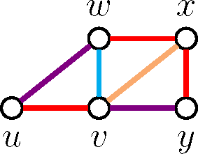
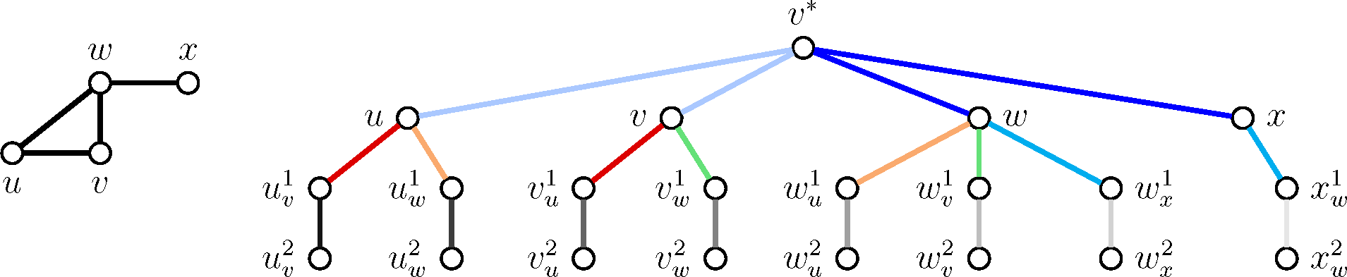
κ by Lemma 5). We construct a MINIMUM RAINBOW SUBGRAPH instance (G′ = (V, E′), χ) as follows; an illustration is given in Figure 2. First, set V′ := V. Then do the following for each edge {u, υ} ∈ E. Add four vertices u υ 1, u υ 2, υ u 1, υ u 2. Make u υ 1 and u υ 2 adjacent and color the edge with some unique color. Analogously, make υ u 1 and υ u 2 adjacent and color the edge with some other unique color. Now, add an edge between u and u υ 1 and an edge between υ and υ u 1. Color both edges with the new color c{u,v}. Finally, add another vertex υ and make υ adjacent to all vertices of V. To color the edges between υ and V, we use the perfect matching M. For each edge {u, υ} of M, we color the edges {υ, u} and {υ, υ} with the same new color C { u , υ } M. The resulting tree has depth three, since every leaf has distance two to a vertex from V and these vertices are all adjacent to υ. Moreover, every color occurs at most twice. It remains to show the following equivalence to obtain a parameterized reduction.
G has an independent set of size κ G has a rainbow subgraph of order : = n κ .
“⇒”: Let S be an independent set of size κ in G. We show that the subgraph G″ obtained by removing S from G′ is rainbow. First, none of the vertices in V is incident with an edge with a unique color, so these edges remain in G″. Moreover, for each edge incident with υ ∈ S in G, there is another edge in G′ that has the same color. The endpoints of this edge are either not in V or they are adjacent to υ in G, so they are not in S. This other edge thus remains in G″.
“⇐”: Let S be a set such that |S| = κ and deleting S′ from G′ results in a rainbow graph G″. The set S has the following properties: First, υ is not in S, since otherwise an edge with color C { u , υ } M is missing in G″. Second, the leaves of G′ and their neighbors are also in G″, since the edges between these vertices have unique colors. Hence, S′ ⊆ V. Clearly, S′ is an independent set in G: If S′ contains two vertices u and υ that are adjacent in G, then both edges with color c{u,v} are missing from G″.□

5.2. Degree and Color-Degree

By Theorem 6, parameterization by alone does not yield fixed-parameter tractability. Hence, we consider combinations of with two parameters. One is the maximum degree Δ, and the other one is the maximum color degree ΔC := maxυ∈V |{c | ∃{u, υ} ∈ E : χ({u, υ}) = c}|, which is the maximum number of colors incident with any vertex in G. This parameter was also considered by Schiermeyer [21] for obtaining bounds on the size of minimum rainbow subgraphs. Note that the maximum color degree is upper-bounded by both the maximum degree and by the number of colors in G and that it may be much smaller than either parameter.
First, we show that for the combined parameter (Δ, ℓ) the problem has a polynomial-size problem kernel. To our knowledge, this is the first non-trivial kernelization result for RAINBOW SUBGRAPH. As it is common for kernelizations, it is based on a set of polynomial-time executable data reduction rules. The main idea of the kernelization is as follows. We first remove edges whose colors appear very often compared to Δ and . Afterwards, deleting any vertex υ “influences” only a bounded number of other vertices: at most Δ edges are incident with υ, and for each of these edges the number of other edges that have the same color depends only on Δ and . We then consider some vertices that are in every rainbow cover. To this end, we call a vertex υ obligatory if there is some edge color such that all edges with this color are incident with υ. In the data reduction rules, we remove those obligatory vertices that have only obligatory neighbors. Together with the previous reduction rules, we then obtain the kernel by the following argument: If there are many non-obligatory vertices, then we can greedily find a solution, since any vertex deletion has bounded “influence”. Otherwise, the overall instance size is bounded as every other vertex is a neighbor of some non-obligatory vertex and each non-obligatory vertex has at most Δ neighbors.
As mentioned above, the first rule removes edges whose color appears very often compared to Δ and . Obviously, when we remove edges from the graph, we also remove their entry from χ.
Rule 1. If there is an edge color c such that there are more than Δℓ edges with color c, then remove all edges with color c from G.
Proof of correctness. Deleting at most vertices from G may destroy at most Δ edges. Hence, any subgraph of order n − ℓ of G contains an edge of color c. Consequently, removing edges of color c from G cannot transform a no-instance into a yes-instance.
We now deal with obligatory vertices. The first simple rule identifies edge colors that are already covered by obligatory vertices.
Rule 2. If G contains an edge {u, υ} of color c such that u and υ are obligatory, then remove all other edges with color c from G.
Proof of correctness. An application of the rule cannot transform a no-instance into a yes-instance, since it removes edges from G without removing the color from G. Assume that the original instance is a yes-instance. Since u and υ are obligatory, any rainbow cover contains u and υ. Therefore, any rainbow cover of the original instance contains an edge with color c and thus it is also a rainbow cover in the new instance, since only edges of color c are deleted. □
We now work on instances that are reduced with respect to Rule 2. Observe that in such instances every edge between two obligatory vertices has a unique color. This observation is crucial for showing the correctness of the following rules. Their aim is to remove obligatory vertices that have only obligatory neighbors. When removing a vertex in these rules, we decrease k and n by one, thus the value of remains the same. The correctness of the first rule is obvious.
Rule 3. Let (G, χ) be an instance that is reduced with respect to Rule 2. Then, remove all connected components of G that consist of obligatory vertices only.
The next two rules remove edges between obligatory vertices.
Rule 4. Let (G, χ) be an instance that is reduced with respect to Rule 2. If G contains three obligatory vertices u, υ, and w such that {u, υ}, {υ, w} ∈ E and u has only obligatory neighbors, then remove {u, υ} from G. If u has degree zero now, then remove u from G.
Proof of correctness. Let (G′ = (V, E′), χ′) denote the instance that is produced by an application of the rule. We show that
G has a rainbow cover of order | V | G has a rainbow cover of order | V | .
“⇒”: If u is not removed by the rule, then this holds trivially as we remove an edge which has a unique color. Otherwise, let S be a vertex set such that G[S] is a rainbow cover. Since u is obligatory, we have uS. The only color incident with u is χ({u, υ}). This color is not present in G′, so the graph G′ [S \ {u}] is a rainbow cover of G′. Since |V| − |V′| = |S| − |S′|, the claim holds also in this case. “⇐”: Let S′ be a set such that G′ [S′] is a rainbow cover of G′. Since G is reduced with respect to Rule 2, υ and w are connected by an edge whose color is unique. Hence, they are obligatory in G′.
If the rule does not remove u from G, then u is also obligatory in G′ since all its neighbors in G′ are obligatory and thus all edges incident with u in G′ have a unique color. Hence, the subgraph G[S′] of G contains all edge colors that are present in both G and G′ plus the color χ({u, υ}). Thus, it is a rainbow cover of G. If the rule removes the vertex u, then the graph G[S] with S = S′ ∪ {u} is a rainbow cover of G: The only color that is in G but not in G′ is χ({u, υ}) which is present in G[S] as S contains u and υ. Again, the claim follows from the fact that |S| − |S′| = |V| − |V′|.
Rule 5. Let (G, χ) be an instance of RAINBOW SUBGRAPH that is reduced with respect to Rule 2. If G = (V, E) contains four obligatory vertices u, υ, w, and x such that {u, υ} ∈ E and {w, x} ∈ E and u and x have only obligatory neighbors, then do the following. Remove {w, x} from G. If υ and w are not adjacent, then insert, w} and assign it a unique color. If x has now degree zero, then remove x from G.
Proof of correctness. Let (G′ = (V, E′), χ′) denote the instance that is produced by an application of the rule. We show that
G has a rainbow cover of order | V | G has a rainbow cover of order | V | .
“⇒”: Let S be a vertex set such that G[S] is a rainbow cover. Clearly, {u, υ, w, x} ⊆ S. First, consider the case that the application of the rule does not remove x. Then, the graph G′ [S] is clearly also a rainbow cover as it contains all edge colors that are in both G and G′ plus possibly the new edge color χ({υ, w}).
Now assume that the rule removes x. In this case, G′ [S′] with S′ := S \ {x} is a rainbow cover by the same arguments. Since |V| − |V′| = |S| − |S′|, the claim holds also in this case.
“⇐”: Let S′ be a set such that G′[S′] is a rainbow cover. If the rule does not remove x from G, then {u, υ, w, x} ⊆ S as these four vertices are obligatory in G′ ({u, υ
} and {υ, w} have unique colors and x has in G′ an obligatory neighbor, so the edge between them is obligatory). Therefore, G[S′] is also a rainbow cover by similar arguments as above. Now assume that the rule removes x from G. In this case {u, υ, w} ⊆ S′ as all three vertices are obligatory in G′. Then, G[S] with S := S′ ∪ {x} is a rainbow cover of G. First, the only color contained in G not in G′ is χ({w, x}), and this color is contained in G[S].
Second, the only edge present in G′[S′] not in G[S] is possibly {υ, w}. If {υ, w} is not in G[S], then there is also no other edge of color χ({υ, w}) in G. Note that |V| − |V′| = |S| − |S′|, so the claim holds also in this case.
Note that application of Rule 4 does not increase the maximum degree of the instance and decreases the degree of υ and w. Furthermore, note that application of Rule 5 may increase the degree of υ by one but directly triggers an application of Rule 4 which reduces the degree of υ and u again by one. Hence, both rules can be exhaustively applied without increasing the overall maximum degree.
We now show that after exhaustive application of the above data reduction rules, the instance has bounded size or otherwise can be solved immediately.
Lemma 6. Let (G, χ) be an instance that is reduced with respect to Rules 1 to 5. Then, (G, χ) is a yes-instance or it contains at most 2Δ·(Δ + 1)·ΔC·2vertices.
Proof. We consider a special type of vertex set that can be safely deleted. To this end, call a vertex set S a colorful packing if
  • no vertex in S is obligatory, and
  • for all u, υ ∈ S the set of colors incident with u is disjoint from the set of colors incident with υ.
Assume that (G, χ) has a colorful packing of size . Then, G − S is a rainbow cover of order k: For each color incident with some vertex υ in S, there are two other vertices in V that are connected by an edge with this color (as υ is not obligatory). By the second condition, these two vertices are not in S. Hence, this edge color is contained in G − S. Summarizing, if (G, χ) contains a colorful packing of size at least , then (G, χ) is a yes-instance.
Now, assume that a maximum-cardinality colorful packing S in G has size less than . Each vertex in S is incident with at most ΔC colors. For each of these colors, the graph induced by the edges of this color has at most Δ edges and thus at most 2Δ vertices, since the instance is reduced with respect to Rule 1.
Let T denote the set of vertices in V \ S that are incident with at least one edge that has the same color as as an edge incident with some vertex in S. By the above discussion,
| T | 2 Δ Δ C ( 1 ) .
Note that T includes all neighbors of vertices in S. By the maximality of S, all vertices in V \ (ST) are obligatory. Now partition V \ (ST) into the set X that has neighbors in T and the set Y that has only neighbors in (XY). The set X has size at most (2ΔC · Δ · ℓ · (ℓ − 1)) · Δ since the maximum degree in G is Δ. The set Y has size at most 1 since otherwise one of the Rules 3 to 5 applies: Every vertex in Y is obligatory and has only obligatory neighbors. If two vertices of Y have a common neighbor, then Rule 4 applies. If G has a connected component consisting only of vertices of Y, then Rule 3 applies. The only remaining case is that Y has two vertices u and x that have different obligatory neighbors in X. In this case, Rule 5 applies. Since S has size at most ℓ − 1, G contains thus at most
1 + 2 Δ Δ C ( 1 ) + 2 Δ 2 Δ C ( 1 ) + 1 < 2 Δ ( Δ + 1 ) Δ C 2
vertices. Hence, if an instance contains more vertices, then it has a colorful packing of size at least , which implies that it is a yes-instance. □
Using Lemma 6, we obtain the following theorem.
Theorem 7. RAINBOW SUBGRAPH admits a problem kernel with at most· (Δ + 1) · ΔC · ℓ2 vertices that can be computed in O(m2 + mn) time.
Proof. The kernelization algorithm exhaustively applies Rules 1 to 5 and then checks whether the instance contains more than 2Δ · (Δ + 1) · ΔC · ℓ2 vertices. If this is the case, then the algorithm answers “yes” (or reduces to a yes-instance of size one) which is correct by Lemma 6 or the instance has bounded size. It remains to show the running time of the algorithm.
Each rule removes at least one edge or, in the case of Rule 5, immediately triggers a rule that removes at least one edge. Hence the rules are applied at most m times. Moreover, the applicability of each rule can be tested in O(m + n) time, which can be seen as follows. Herein, we only focus on the time needed to test the condition of the rules; the modifications can be clearly performed in linear time. For Rule 1, one needs only to count the number of occurrences of an edge color, which can be done by visiting each edge and using an array of size p to count the occurrences. For Rule 2, one must first determine the set of obligatory vertices in O(m + n) time by comparing the number of incident edges for each color to the previously computed total number of edges with this color. Then, visiting each edge of G, one can check in constant time whether both endpoints are obligatory. Rule 3 can clearly be performed in linear time by computing the connected components of G. Rule 4 can be performed in linear time by checking for each obligatory vertex whether it has degree at least two and only obligatory neighbors. Finally, Rule 5 can be performed in linear time as follows. First, the set of obligatory vertices with only obligatory neighbors is already computed by the algorithm for Rule 4. Then, one can remove in linear time all edges that do not have at least one endpoint that is obligatory and has only obligatory neighbors. In the remaining graph, compute in linear time a matching of size two. This matching fulfills the requirements of Rule 5; if there is no such matching, then Rule 5 does not apply. Altogether, the running time of the kernelization algorithm is O(m2 + mn). □
We now consider parameterization by (ΔC, ℓ) (recall that the color degree ΔC can be much smaller than Δ). First, by performing the following additional data reduction rule, we can use the kernelization result for (Δ, ℓ) to obtain a polynomial problem kernel for (ΔC, ℓ).
Rule 6. If G contains a vertex υ such that at least ℓ + 2 edges incident with υ have the same color c, then delete an arbitrary one of these edges.
Proof of correctness. Clearly, we cannot transform a no-instance into a yes-instance, since the color c remains in the graph after application of the rule. If (G, χ) is a yes-instance, then there is an order-(n − ℓ) rainbow cover of G that contains at least two vertices that are in G connected to υ by an edge with color c. Hence, removing at most one of these two edges does not destroy the rainbow cover. □
Rule 6 can be exhaustively performed in linear time: For each vertex υ, scan through its adjacency list, counting the number of incident edges of each color in an array of size p. When encountering an edge whose color counter is + 2, immediately delete the edge; otherwise increment the counter. Afterwards, reset the array to contain only zero entries; this can be done in O(deg(υ)) time by storing a list of edge colors that are incident with υ (all other entries of the array have the value zero, so only these counters have to be reset). Finally, the rule does not change the value of , so each vertex needs to be visited only once.
After exhaustive application of the rule, the maximum degree Δ of G is at most ΔC · ( + 1). In combination with Theorem 7, this immediately implies the following.
Theorem 8. RAINBOW SUBGRAPH has a problem kernel with at most 2(ΔC + 1)3 2( + 1)2 vertices that can be computed in O(m2 + mn) time.
Finally, we describe a simple branching for the parameter (ΔC, ℓ). Herein, deleting a vertex means to remove it from G and to decrease by one; thus, a deleted vertex is not part of a rainbow cover of order k of the original instance.
Branching Rule 1. If G contains a non-obligatory vertex u, then branch into the following cases. First, recursively solve the instance obtained from deleting u from G. Then, for each color c that is incident with u pick an edge {v, w} with color c. If υ (w) is non-obligatory, then recursively solve the instance obtained from deleting υ (w).
Proof of correctness. We show that
( G , χ ) is a yes-instance one of the created instances is a yes-instance .
“⇒”: Consider some maximum-cardinality set S such that |S| ≥ ℓ and G − S is a rainbow cover of G. If S contains any of the vertices υ and w considered in the second part of the branching, then the claim holds. Otherwise, for each color c that is incident with u, there is an edge in G − S that has color c. In this case, we can assume uS since S has maximum cardinality, so the claim also holds in this case.
“⇐”: Consider any instance (G, χ′) created during the branching and let S denote a set of at least ℓ −1 vertices such that G− S is a rainbow cover of G′. Let υ denote the vertex that is in G′ but not in G. Since υ is non-obligatory, all colors in G are also present in G′. Hence, G (S ∪ {v}) is also a rainbow cover of G. Hence, (G, χ) is also a yes-instance. □
Note that the parameter decreases by one in each branch. Exhaustively applying Branching Rule 1 until either every vertex is obligatory or ℓ ≤ 0 yields an algorithm with the following running time.
Theorem 9. RAINBOW SUBGRAPH can be solved in O((2ΔC + 1) · (n + m)) time.
Proof. The algorithm exhaustively applies Branching Rule 1 until either every vertex is obligatory or ℓ ≤ 0. By the correctness of Branching Rule 1 the original instance is a yes-instance if and only if at least one of the created instances is a yes-instance.
If = 0, then the instance is a trivial yes-instance and the algorithm may correctly answer “yes”. Otherwise, > 0 but all vertices are obligatory. In this case, the instance is a trivial no-instance and the algorithm simply leaves the current branch. If the answer for none of the created instances is “yes”, then the algorithm correctly answers “no”.
It remains to show the running time bound. The search tree created by Branching Rule 1 has depth and maximum degree (2ΔC + 1), hence it has size O((2ΔC + 1)). In each node of the instance, we have to test for the applicability of Branching Rule 1, which can be performed in linear time. □

6. Outlook

Considering its biological motivation, it would be interesting to gain further, potentially data-driven parameterizations of MINIMUM RAINBOW SUBGRAPH that may help identifying further practically relevant and tractable special cases. An interesting parameter which we have not investigated so far is the combination (ΔC, k) of solution order and maximum color degree. From a more graph-theoretic point of view, we left open a deeper study of parameters measuring the degree of acyclicity of the underlying graph, such as treewidth or feedback set numbers. It also remains open whether there are polynomial-space fixed-parameter algorithms for the parameters (Δ, k) and (Δ, p).

Acknowledgments

We thank the anonymous reviewers of WG 2014 and of Algorithms for their thorough and valuable feedback. In particular, an anonymous reviewer of Algorithms pointed out a substantial simplification of Section 4.2. Falk Hüffner was supported by DFG project ALEPH (HU 2139/1), and Christian Komusiewicz was partially supported by a post-doctorial grant funded by the Région Pays de la Loire.

Author Contributions

All authors contributed equally.

Conflicts of Interest

The authors declare no conflicts of interest.

References

  1. Hajiaghayi, M.T.; Jain, K.; Lau, L.C.; Mandoiu, I.I.; Russell, A.; Vazirani, V.V. Minimum multicolored subgraph problem in multiplex PCR primer set selection and population haplotyping, Proceedings of the 6th International Conference on Computational Science (ICCS ’06), Reading, UK, 28–31 May 2006; Springer Berlin Heidelberg: Berlin, Germany, 2006; pp. 758–766.
  2. Matos Camacho, S.; Schiermeyer, I.; Tuza, Z. Approximation algorithms for the minimum rainbow subgraph problem. Discret. Math. 2010, 310, 2666–2670. [Google Scholar]
  3. Fernandes, R.; Skiena, S. Microarray synthesis through multiple-use PCR primer design. Bioinformatics 2002, 18, 128–135. [Google Scholar]
  4. Katrenič, J.; Schiermeyer, I. Improved approximation bounds for the minimum rainbow subgraph problem. Inf. Proc. Lett. 2011, 111, 110–114. [Google Scholar]
  5. Popa, A. Better lower and upper bounds for the minimum rainbow subgraph problem. Theor. Comput. Sci. 2014, 543, 1–8. [Google Scholar]
  6. Koch, M.; Matos Camacho, S.; Schiermeyer, I. Algorithmic approaches for the minimum rainbow subgraph problem. Electron. Notes Discret. Math. 2011, 38, 765–770. [Google Scholar]
  7. Sharan, R.; Halldórsson, B.; Istrail, S. Islands of tractability for parsimony haplotyping. IEEE/ACM Trans. Comput. Biol. Bioinform. 2006, 3, 303–311. [Google Scholar]
  8. Fleischer, R.; Guo, J.; Niedermeier, R.; Uhlmann, J.; Wang, Y.; Weller, M.; Wu, X. Extended islands of tractability for parsimony haplotyping, Proceedings of the 21st Annual Symposium on Combinatorial Pattern Matching (CPM ’10), New York, NY, USA, 21–23 June 2010; Springer Berlin Heidelberg: Berlin, Germany, 2010; pp. 214–226.
  9. Fellows, M.; Hartman, T.; Hermelin, D.; Landau, G.; Rosamond, F.; Rozenberg, L. Haplotype inference constrained by plausible haplotype data. IEEE/ACM Trans. Comput. Biol. Bioinform. 2011, 8, 1692–1699. [Google Scholar]
  10. Hassin, R.; Segev, D. The set cover with pairs problem, Proceedings of the 25th International Conference on Foundations of Software Technology and Theoretical Computer Science (FSTTCS ’05), Hyderabad, India, 15–18 December 2005; Springer Berlin Heidelberg: Berlin, Germany, 2005; pp. 164–176.
  11. Williamson, D.P.; Shmoys, D.B. The Design of Approximation Algorithms; Cambridge University Press: Cambridge, UK, 2011. [Google Scholar]
  12. Downey, R.G.; Fellows, M.R. Fundamentals of Parameterized Complexity; Springer: New York, NY, USA, 2013. [Google Scholar]
  13. Flum, J.; Grohe, M. Parameterized Complexity Theory; Springer Berlin Heidelberg: Berlin, Germany, 2006. [Google Scholar]
  14. Niedermeier, R. Invitation to Fixed-Parameter Algorithms; Oxford University Press: Oxford, UK, 2006. [Google Scholar]
  15. Alimonti, P.; Kann, V. Some APX-completeness results for cubic graphs. Theor. Comput. Sci. 2000, 237, 123–134. [Google Scholar]
  16. Fellows, M.; Hermelin, D.; Rosamond, F.; Vialette, S. On the parameterized complexity of multiple-interval graph problems. Theor. Comput. Sci. 2009, 410, 53–61. [Google Scholar]
  17. Komusiewicz, C.; Sorge, M. Finding dense subgraphs of sparse graphs, Proceedings of the 7th International Conference on Parameterized and Exact Computation (IPEC ’12), Ljubljana, Slovenia, 12–14 September 2012; Springer Berlin Heidelberg: Berlin, Germany, 2012; pp. 242–251.
  18. Björklund, A.; Husfeldt, T.; Koivisto, M. Set partitioning via inclusion-exclusion. SIAM J. Comput. 2009, 39, 546–563. [Google Scholar]
  19. Björklund, A.; Husfeldt, T.; Kaski, P.; Koivisto, M. Fourier meets Möbius: Fast subset convolution, Proceedings of the 39th Annual ACM Symposium on Theory of Computing (STOC ’07), San Diego, CA, USA, 11–13 June 2007; ACM: New York, NY, USA, 2007; pp. 67–74.
  20. Fürer, M. Faster integer multiplication, Proceedings of the 39th Annual ACM Symposium on Theory of Computing (STOC ’07), San Diego, CA, USA, 11–13 June 2007; ACM: New York, NY, USA, 2007; pp. 57–66.
  21. Schiermeyer, I. On the minimum rainbow subgraph number of a graph. Ars Math. Contemp. 2012, 6, 83–88. [Google Scholar]
Figure 1. An edge-colored graph G with p = 4 edge colors. The subgraph G′ := G[{u, υ, w, x}] is a rainbow cover. The graph obtained from G′ by removing the red edge {u, υ} is a solution.
Algorithms 08 00060f1
Figure 2. The reduction for showing the W[1]-hardness of RAINBOW SUBGRAPH for parameter . The graph of the INDEPENDENT SET WITH PERFECT MATCHING instance (shown on the left) has a perfect matching {{u, υ}, {w, x}}. Accordingly, the four edges from υ* to V are colored with two colors. The unique colors between the additional vertices which are not from V are shown in shades of gray.
Algorithms 08 00060f2
Table 1. Complexity overview for RAINBOW SUBGRAPH. The O()-notation suppresses factors polynomial in the input size; — ” — denotes that a result follows from the entry above. Some results are inferred by parameter relations Equations (1), (2), or (3) (see Section 2).
Par.PathsTreesGeneral Graphs
pO*(2p) (Theorem 5)O*(2p) (Theorem 5)W[1]-hard (Theorem 2)
p, Δ—”——”—O*((4Δ − 4)p) (Theorem 3)

kO* (2k) (Theorem 5 + Equation (2))O* (2k) (Theorem 5 + Equation (3))W[1]-hard (Theorem 2 + Equation (1))
k, Δ—”——”—O*(2kΔ/2) (Theorem 4)

O*(5) (Theorem 9)W[1]-hard (Theorem 6)W[1]-hard (Theorem 6)
, Δ—”—O*((2Δ + 1)) (Theorem 9)O*((2Δ + 1)) (Theorem 9)
O32)-vertex kernel (Theorem 7)
, ΔC—”—O*((2ΔC + 1)) (Theorem 9)O*((2ΔC + 1)) (Theorem 9)
O ( Δ C 3 4 )-vertex kernel (Theorem 8)
ℓ, q—”—W[1]-hard (Theorem 6)W[1]-hard (Theorem 6)

q, ΔAPX-hard (Theorem 1)APX-hard (Theorem 1)APX-hard [4]

