Characterizing functional connectivity differences in aging adults using machine learning on resting state fMRI data
- 1Medical Physics, University of Wisconsin–Madison, Madison, WI, USA
- 2Clinical Neuroengineering Training Program, University of Wisconsin–Madison, Madison, WI, USA
- 3Radiology, University of Wisconsin–Madison, Madison, WI, USA
- 4Electrical and Computer Engineering, University of Wisconsin–Madison, Madison WI, USA
- 5Neuroscience Training Program, University of Wisconsin–Madison, Madison, WI, USA
- 6Biomedical Engineering, University of Wisconsin–Madison, Madison, WI, USA
- 7Medicine and Biostatistics, University of Pittsburgh, Pittsburgh, PA, USA
- 8Biostatistics and Medical Informatics, University of Wisconsin–Madison, Madison, WI, USA
- 9Radiology, New Jersey Medical School, Newark, NJ, USA
- 10Waisman Center, University of Wisconsin–Madison, Madison, WI, USA
- 11Psychiatry, University of Wisconsin–Madison, Madison, WI, USA
- 12Psychology, University of Wisconsin–Madison, Madison, WI, USA
The brain at rest consists of spatially distributed but functionally connected regions, called intrinsic connectivity networks (ICNs). Resting state functional magnetic resonance imaging (rs-fMRI) has emerged as a way to characterize brain networks without confounds associated with task fMRI such as task difficulty and performance. Here we applied a Support Vector Machine (SVM) linear classifier as well as a support vector machine regressor to rs-fMRI data in order to compare age-related differences in four of the major functional brain networks: the default, cingulo-opercular, fronto-parietal, and sensorimotor. A linear SVM classifier discriminated between young and old subjects with 84% accuracy (p-value < 1 × 10⁻⁷). A linear SVR age predictor performed reasonably well in continuous age prediction (R2 = 0.419, p-value < 1 × 10⁻⁸). These findings reveal that differences in intrinsic connectivity as measured with rs-fMRI exist between subjects, and that SVM methods are capable of detecting and utilizing these differences for classification and prediction.
Introduction
Functional networks are defined by a temporal correlation of brain regions normally involved during a task and are observed when individuals are resting without performing a specific task (Biswal et al., 1995).
Research efforts in functional magnetic resonance imaging (fMRI) are shifting focus from studying specific cognitive domains like vision, language, memory, and emotion to assessing individual differences in neural connectivity across multiple whole-brain networks (Thomason et al., 2011). Subsequently, an increasing number of studies using rs-fMRI data, are showing reproducibility and reliability (Damoiseaux et al., 2006; Shehzad et al., 2009; Van Dijk et al., 2010; Zuo et al., 2010; Thomason et al., 2011; Song et al., 2012), for studying functional connectivity of the human brain.
Simultaneously, use of machine learning techniques for analyzing fMRI data has increased in popularity. In particular, Support Vector Machines (SVMs) have become widely used due to their ability to handle very high-dimensional data and their classification and prediction accuracy (Schölkopf and Smola, 2002; Ben-Hur and Weston, 2010; Meier et al., 2012). Various fMRI data analysis methods are currently used including seed-based analysis, independent component analysis (ICA), graph theory methods, but in this work we chose SVMs because they, unlike the others, offer the ability to classify and predict individual scans and output relevant features. A growing number of studies have shown that machine learning tools can be used to extract exciting new information from neuroimaging data (see Haynes and Rees, 2005; Norman et al., 2006; Cohen et al., 2011 for selective reviews).
With task-based fMRI data, LaConte et al. (2007) observed 80% classification accuracy of real-time brain state prediction using a linear kernel SVM on whole-brain, block-design, motor data and Poldrack et al. (2009) achieved 80% classification accuracy of predicting eight different cognitive tasks that an individual performed using a multi-class SVM (mcSVM) method.
Resting state fMRI data has been shown viable in classification and prediction. Craddock et al. (2009) used resting state functional connectivity MRI (rs-fcMRI) data to successfully distinguish between individuals with major depressive disorder from healthy controls with 95% accuracy using a linear classifier with a reliability filter for feature selection. Supekar et al. (2009) classified individuals as children or young-adults with 90% accuracy using a SVM classifier. Shen et al. (2010) achieved 81% accuracy for discrimination between schizophrenic patients and healthy controls using a SVM classifier and achieved 92% accuracy using a C-means clustering classifier with locally linear embedding (LLE) feature selection. Dosenbach et al. (2010), using a SVM method, achieved 91% accuracy for classification of individuals as either children or adults, and also predicted functional maturity for each participant’s brain using support vector machine regression (SVR).
One advantage of resting state data as opposed to task-based data is that the acquiring of resting data is not constrained by task difficulty and performance. This provides a potentially larger group of subjects that are not able to perform tasks (e.g., Alzheimer’s Disease patients, patients with severe stroke) on which studies can be done. There has been a great amount of progress made in describing typical and atypical brain activity at the group level with the use of fMRI, but, determining whether single fMRI scans contain enough information to classify and make predictions about individuals remains a critical challenge (Dosenbach et al., 2010). Our method builds on the classification and prediction of individual scans using multivariate pattern recognition algorithms, adding to this currently novel domain in the literature.
We describe a classification and regression method implemented on aging adult rs-fcMRI data using SVMs, extracting relevant features, and building on the SVM/SVR study of children to middle-aged subjects (Dosenbach et al., 2010) and aging adults (Meier et al., 2012). SVM has been applied to a wide range of datasets, but has only recently been applied to neuroimaging-fMRI data, especially resting fMRI data which is still relatively novel. This work expands upon and adds to the relatively new literature of resting fMRI based classification and prediction. Our objective was to investigate the ability of the SVM classifier to discriminate between individuals with respect to age and the ability of the SVR predictor to determine individuals’ age using only functional connectivity MRI data. Beyond binary SVM classification and SVR prediction, our work investigates multi-class classification and linear weights for evaluating feature importance of healthy aging adults.
Materials and Methods
Participants
Resting state data for 65 individuals (three scans each) were obtained from the ICBM dataset made freely accessible online by the 1000 Connectome Project1. Each contributor’s respective ethics committee approved submission of the de-identified data. The institutional review boards of NYU Langone Medical Center and New Jersey Medical School approved the receipt and dissemination of the data (Biswal et al., 2010).
Data Sets
The analyses described in this work were performed on two data sets contained in the ICBM set. The same preprocessing algorithms were applied to both sets of data.
Data set 1 consisted of 52 right-handed individuals (age 19–85, mean 44.7, 23M/29F). This was the binary SVM set (both for age and gender classification) which contained a young group of 26 subjects (age 19–35, mean 24.7, 12M/14F) and an old group of 26 subjects (age 55–85, mean 64.7, 11M/15F).
Data set 2 consisted of 65 right-handed individuals (ages 19–85, mean 44.9, 32M/33F). This was the mcSVM set as well as the SVR age prediction set. It contained three age groups used for mcSVM: a young group of 28 subjects (age 19–37, mean 25.5, 14M/14F), a middle-aged group of 22 subjects (age 42–60, mean 52.4, 11M/11F), and an old group of 15 subjects (age 61–85, mean 69.9, 7M/8F).
Data Acquisition
Resting data were acquired with a 3.0 Tesla scanner using an echo planar imaging (EPI) pulse sequence. Three resting state scans were obtained for each participant, and consisted of 128 continuous resting state volumes (TR = 2000 ms; matrix = 64 × 64; 23 axial slices). Scan 1 and 3 had an acquisition voxel size = 4 mm × 4 mm × 5.5 mm, while scan 2 had an acquisition voxel size = 4 mm × 4 mm × 4 mm. All participants were asked to keep their eyes closed during the scan. For spatial normalization and localization, a T1-weighted anatomical image was acquired using a magnetization prepared gradient echo sequence (MP-RAGE, 160 sagittal slices, voxel size = 1 mm × 1 mm × 1 mm).
Data Preprocessing
Data were preprocessed using AFNI (version AFNI_2009_12_31_14312), FSL (version 4.1.43), and the NITRC 1000 functional connectome preprocessing scripts made freely available online (version 1.14) (Neuroimaging Informatics Tools and Resources Clearinghouse (NITRC), 2011). Initial preprocessing using AFNI consisted of (1) slice time correction for interleaved acquisition using Fourier-space time series phase-shifting, (2) motion correction of time series by aligning each volume to the mean image using Fourier interpolation, (3) skull stripping, and (4) getting an eighth image for use in registration. Preprocessing using FSL consisted of (5) spatial smoothing using a Gaussian kernel of full-width half maximum = 6 mm, and (6) grand-mean scaling of the voxel values. The data were then temporally filtered (0.005–0.1 Hz) and detrended to remove linear and quadratic trends using AFNI. A mask of preprocessed data for each person was generated.
Nuisance Signal Regression
Nuisance signal [white matter, cerebrospinal fluid (CSF) and six motion parameters] was then removed from the preprocessed fMRI data. White matter and CSF masks were created using FSL by the segmentation of each individual’s structural image. These masks were then applied to each volume to remove the white matter and CSF signal. Following the removal of these nuisance signals, functional data were then transformed into Montreal Neurological Institute 152 (MNI152-brain template; voxel size = 3 mm × 3 mm × 3 mm) space using a two-step process. First a 6 degree-of-freedom affine transform was applied using FLIRT (Smith et al., 2004) to align the functional data into anatomical space. Then, the anatomical image was aligned into standard MNI space using a 12 degree-of-freedom affine transform implemented in FLIRT. Finally, the resulting transform was then applied to each subject’s functional dataset.
ROI Based Functional Connectivity
One hundred functionally defined regions of interest (ROIs) encompassing the default mode, cingulo-opercular, fronto-parietal, and sensorimotor networks (see Figure 1), were selected in agreement with a previous study by Dosenbach et al. (2010) and Meier et al. (2012). Each ROI was defined by a sphere (radius = 5 mm) centered about a three-dimensional point with coordinates reported in MNI space.
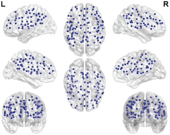
Figure 1. Functional ROIs used in the study. Each ROI is spherical with a 5 mm radius.
Average resting state blood oxygenation level dependent (BOLD) time series for each ROI were extracted. The BOLD time series for each ROI were then correlated with the BOLD time series of every other ROI (Pearson’s correlation) for every subject and every scan. This resulted in a square (100 × 100) symmetric matrix of correlation coefficients for each scan, but only 4950 ROI-pair correlation values from the lower triangular part of the matrix were retained (redundant elements and diagonal elements were excluded). These were then z-transformed (Fisher’s z transformation) for normalization. These 4950 values of the functional connectivity matrix were subsequently used as features in the SVM and SVR methods. Figure 2 shows a series of steps in a representative pipeline of the classification method.
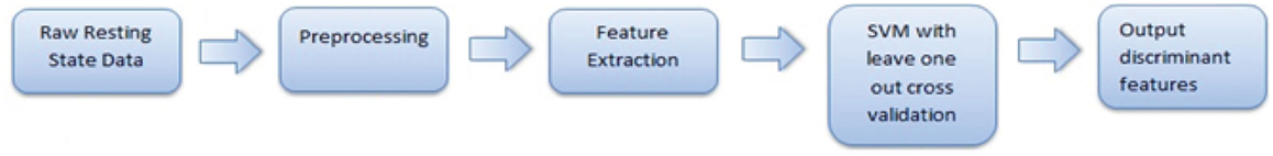
Figure 2. Pipeline of the classification method.
Support Vector Machine Classification and Regression
The SVM is a widely used classification method due to its favorable characteristics of high accuracy, ability to deal with high-dimensional data and versatility in modeling diverse sources of data (Schölkopf et al., 2004). We chose this method of classification due to its sensitivity, resilience to overfitting, ability to extract and interpret features, and recent history of impressive neuroimaging results (Mitchell et al., 2008; Soon et al., 2008; Johnson et al., 2009; Dosenbach et al., 2010; Schurger et al., 2010; Meier et al., 2012).
A SVM is an example of a linear two-class classifier, which is based on a linear discriminant function:
The vector w is the weight vector, b is called the bias and xi is the i-th example in the dataset. In our study we have a dataset of n examples each of p retained features, xi ∈ ℝp, where n is the number of subjects and p is the number of retained ROI-pair correlation values after t-test filtering. Each example xi has a user defined label yi = +1 or −1, corresponding to the class that it belongs to. In this work binary participant classes are young or old and male or female subjects.
A brief description of the SVM optimization problem is given here and a more detailed one can be found in Vapnik’s (1995) work and Schölkopf and Smola (2002). For linearly separable data, a hard margin SVM classifier is a discriminant function that maximizes the geometric margin, which leads to the following constrained optimization problem:
In the soft margin SVM (Cortes and Vapnik, 1995), where misclassification and non-linearly separable data are allowed, the problem constraints can be modified to:
where ξi ≥ 0 are slack variables that allow an example to be in the margin (0 ≤ ξi ≤ 1), or to be misclassified (ξi > 1). The optimization problem, with an additional term that penalizes misclassification and within margin examples, becomes:
The constant C > 0 allows one to control the relative importance of maximizing the margin and minimizing the amount of discriminating boundary and margin slack.
This can be represented in a dual formulation in terms of variables αi (Cortes and Vapnik, 1995):
The dual formulation leads to an expansion of the weight vector in terms of input data examples:
The examples xi for which αi > 0 are within the margin and are called support vectors.
The discriminant function then becomes:
The dual formulation of the optimization problem depends on the data only through dot products. This dot product can be replaced with a non-linear kernel function, k(x i, xj), enabling margin separation in the feature space of the kernel. Using a different kernel, in essence, maps the example points, xi, into a new high-dimensional space (with the dimension not necessarily equal to the dimension of the original feature space). The discriminant function becomes:
Some commonly used kernels are the polynomial kernel and the Gaussian kernel. In this work we used a linear kernel and a Gaussian kernel, which is also called a radial basis function (RBF):
We tuned the value of C using a holdout subset of the respective dataset. Soft margin binary SVM classification was carried out using the Spider Machine Learning environment (Weston et al., 2005) as well as custom scripts run in MATLAB (R2010a; MathWorks, Natick, MA, USA). Multi-class classification was also carried out using the Spider Machine Learning environment (Weston et al., 2005) utilizing an algorithm, developed by Weston and Watkins (1998), that considers all data at once and solves a single optimization problem.
With some datasets higher classification accuracies can be obtained with the use of non-linear discriminating boundaries (Ben-Hur and Weston, 2010). Using a different kernel maps the data points into a new high-dimensional space, and in this space the SVM discriminating hyperplane is found. Consequently, in the original space, the discriminating boundary will not be linear. All SVM classification and SVR prediction in this work used a linear kernel or a non-linear RBF kernel.
Drucker et al. (1997) extended the SVM method to include SVM regression (SVR) in order to make continuous real-valued predictions. SVR retains some of the main features of SVM classification, but in SVM classification a penalty is observed for misclassified data points, whereas in SVR a penalty is observed for points too far from the regression line in high-dimensional space (Dosenbach et al., 2010).
Epsilon-insensitive SVR defines a tube of width ε, which is user defined, around the regression line in high-dimensional space. Any points within this tube carry no loss. In essence, SVR performs linear regression in high-dimensional space using epsilon-insensitive loss. The C parameter in SVR controls the trade-off between how strongly points beyond the epsilon-insensitive tube are penalized and the flatness of the regression line (larger values of C allow the regression line to be less flat) (Dosenbach et al., 2010). SVR predictions described in this work used epsilon-insensitive SVRs carried out in The Spider Machine Learning environment (Weston et al., 2005), as well as custom scripts run in MATLAB (R2010a; MathWorks, Natick, MA, USA). The parameters C and ε were tuned using a holdout subset of the respective dataset.
Cross Validation
We used leave-one-out-cross-validation (LOOCV) to estimate the SVM classification and SVR prediction accuracy since it is a method that gives the most unbiased estimate of test error (Hastie et al., 2001). In LOOCV the same dataset can be used for both the training and testing of the classifier. The SVM parameters: C and the number of top features, were tuned using a holdout set with LOOCV.
In a round, or fold, of LOOCV, an example from the example set is left out and is used as the entire testing set, while the remaining examples are used as the training set. So each example is left out only once and the number of folds is equal to the number of examples. In our work, LOOCV was performed across participants, not scans, so three scans per participant were removed in each fold and used only in the testing set to avoid “twinning” bias.
T-Test and Correlation Filter
During each SVM LOOCV fold, two-sample t-tests (not assuming equal variance) were run on every feature of the two classes of the training set and the number of features (selected to maximize accuracy) that had the highest absolute t-statistics were selected for use in the classifier. Analogously, during each SVR LOOCV fold, the correlation between each feature and the independent variable (age) was computed, and the features that had the highest absolute correlation values were selected for use in the predictor.
SVM and SVR Feature Weights
One important aspect of SVM and SVR is the determination of which features in the model are most significant with respect to example classification and prediction.
For linear kernel SVM and SVR features, the individual weights of the features as given by the SVM or SVR revealed their relative importance and contribution to the classification or prediction. In the linear kernel SVM and SVR method each node’s (ROI’s) significance, as opposed to each feature’s significance, was directly proportional to the sum of the weights of the connections to and from that node.
Feature and Node Visualization
Feature connections and nodes were visualized using BrainNet Viewer (Version 1.15).
Parameter Tuning
Dosenbach et al. (2010) chose C = 1, top features = 200 for their SVM method and ε = 0.00001, top features = 200 for their SVR method since previous work on a subset of the data revealed that these values provided highest accuracy. Our functional connectivity features used 100 ROIs instead of 160 and this resulted in a different feature space than the one used in the aforementioned study. To tune our SVM parameters for our feature space, we selected a randomly chosen subset, a holdout set, of the respective dataset and chose parameters that maximized classification accuracy and prediction performance for this set.
A holdout set of 20 randomly chosen subjects was used to tune the SVM age and gender classification parameters. We limited ourselves to number of features <1000 for two reasons: previous work (Dosenbach et al., 2010) achieved highest accuracy for features on the order of 100, and this order provides a suitable number of features for characterizing the most relevant brain networks. A “grid search” like method (Hsu et al., 2010) was performed for an interval of number of top features ranging from 20 to 300 to output accuracy as a function of the number of top features and C (see Figure 3). The number of features and value of C that maximized accuracy were used in the total dataset SVM method.
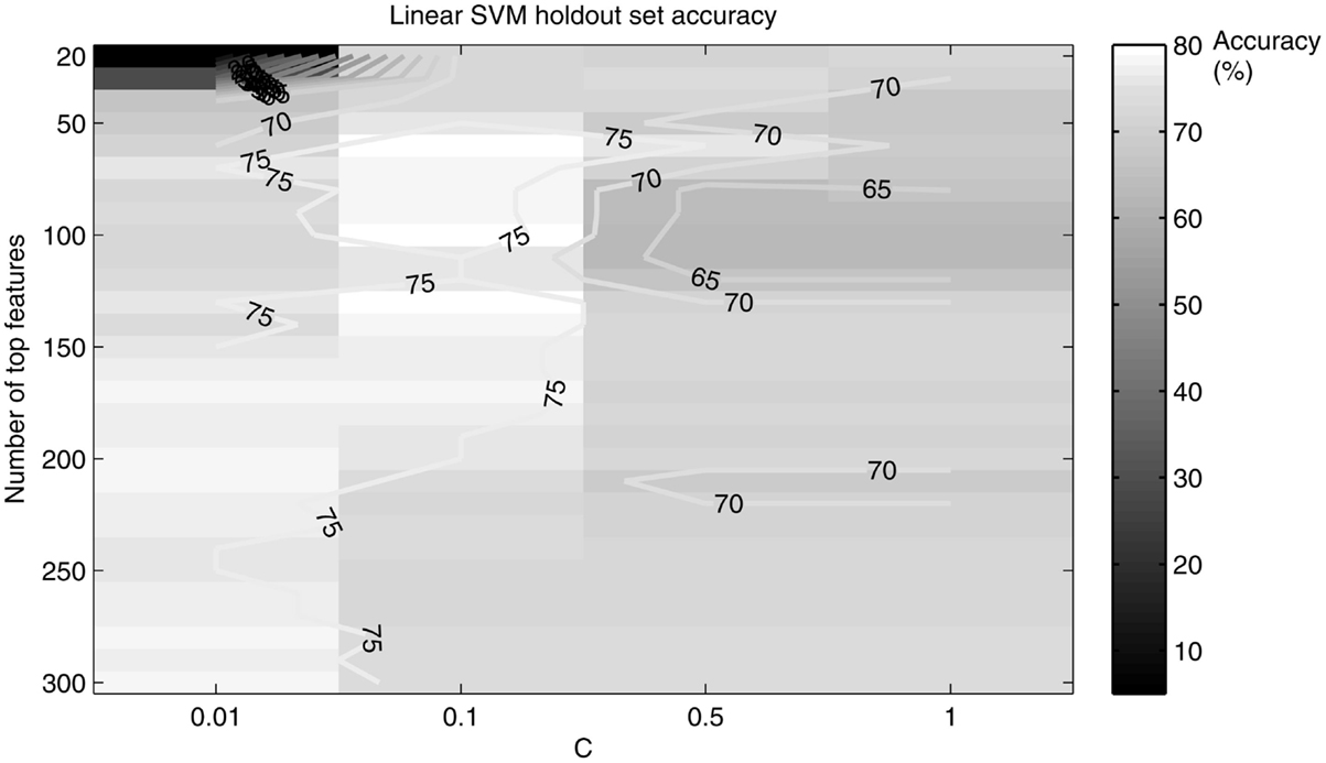
Figure 3. A grid search plot of the hold out set linear SVM age classifier accuracy, as a function of the number of top features and C. Accuracy peaks at 80% for top features retained = 100 and C = 0.1.
A similar procedure for the SVR method was taken. A holdout set of 25 randomly chosen subjects was used to tune the SVR age prediction parameters. First, slope (of a linear regression line fitting the predicted age) as a function of top features was computed to reveal a peak performance area. Then, slope as a function of the number of features and ε was output with a grid search method. The number of features and value of ε that maximized the slope and R2 were used in the total dataset SVR method, where R2 (in this simple linear regression model) is the squared correlation between the predicted and true age. The slope and R2 of a regression line were chosen as measures of performance since a perfect predictor would produce a regression line of the closer the slope and R2 approached one the better the predictor was considered to be.
Results
Support Vector Machine
The binary SVM classifier, using a linear kernel, was able to significantly discriminate between young and old subjects with 84% accuracy (p-value < 1 × 10⁻⁷, binomial test). Chance performance of the classifier would have yielded an accuracy of 50% (the null hypothesis). Therefore, we treated each fold of the LOOCV as a Bernoulli trial with a success probability of 0.5, as specified by Pereira et al. (2009). The p-value is then calculated using the binomial distribution with n trials (n = number of subjects) and probability of success equal to 0.5 as follows: p-value = Pr(X ≥ number of correct classifications), where X is the binomially distributed random variable.
The linear kernel SVM classifier outperformed the RBF kernel SVM classifier with this dataset and a comparison of the two classifiers is given in Table 1. Figure 3 shows how the linear SVM classification accuracy varied with the number of top features retained in the t-test filter as well as how the accuracy varied as a function of the C parameter. The RBF SVM accuracy was 81% with 62 top features retained and C = 1.
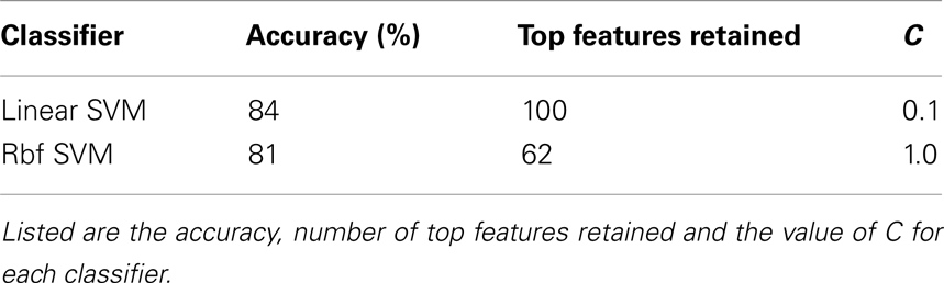
Table 1. A comparison of the two kernel classifiers used for age classification.
Of the 100 total features retained per fold, 63 were present in every fold and these are called the consensus features. Table 2 lists the consensus features and their relative weights or contributions to the classifier; they are also represented in Figure 4. A summation of all of the weights of the connections from each node was performed and the node weights are listed in Table 3 and represented in Figure 5.
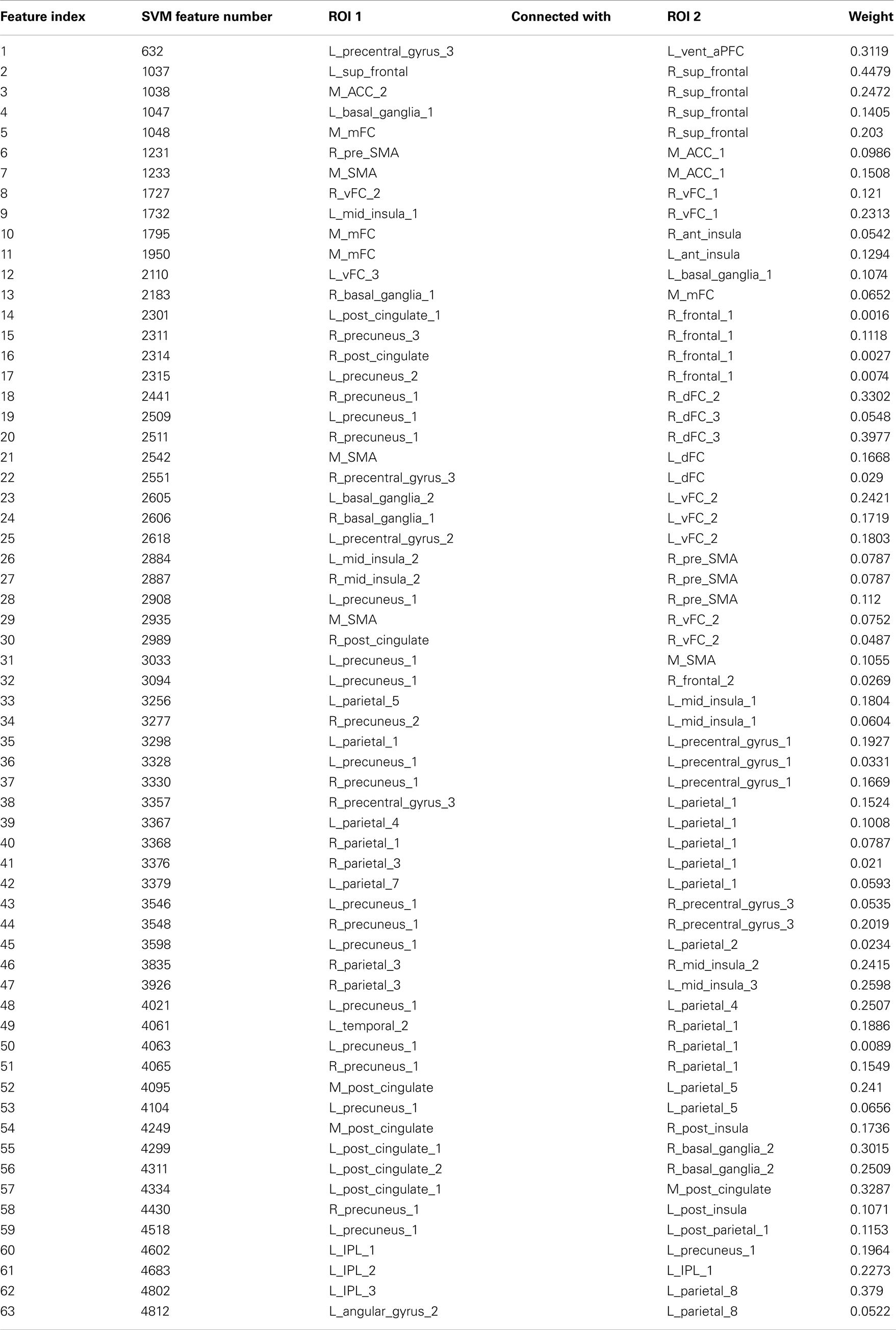
Table 2. List of the 63 consensus features, their node connections and weights for the linear SVM classifier.
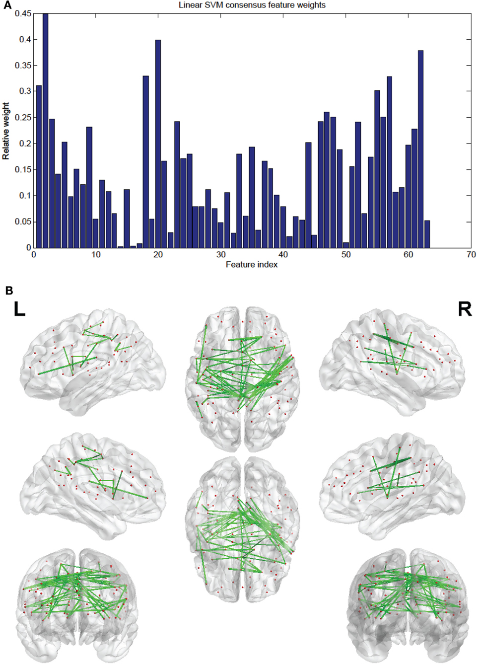
Figure 4. (A) Shows a bar graph representation of the relative weight of each of the 63 consensus features. (B) Shows a representation of the consensus features revealing location using BrainNet Viewer software. Each connection thickness is proportional to the feature weight.
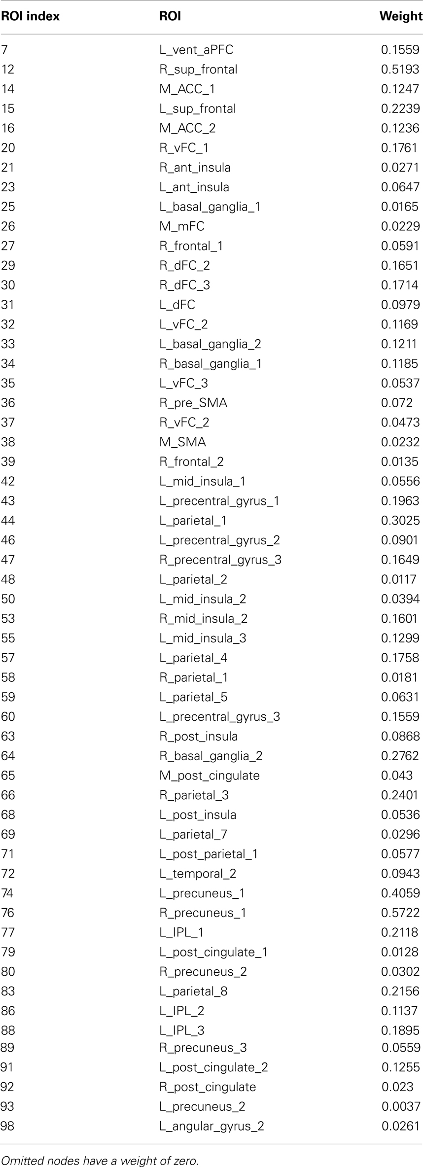
Table 3. Linear SVM nodes and their weights.
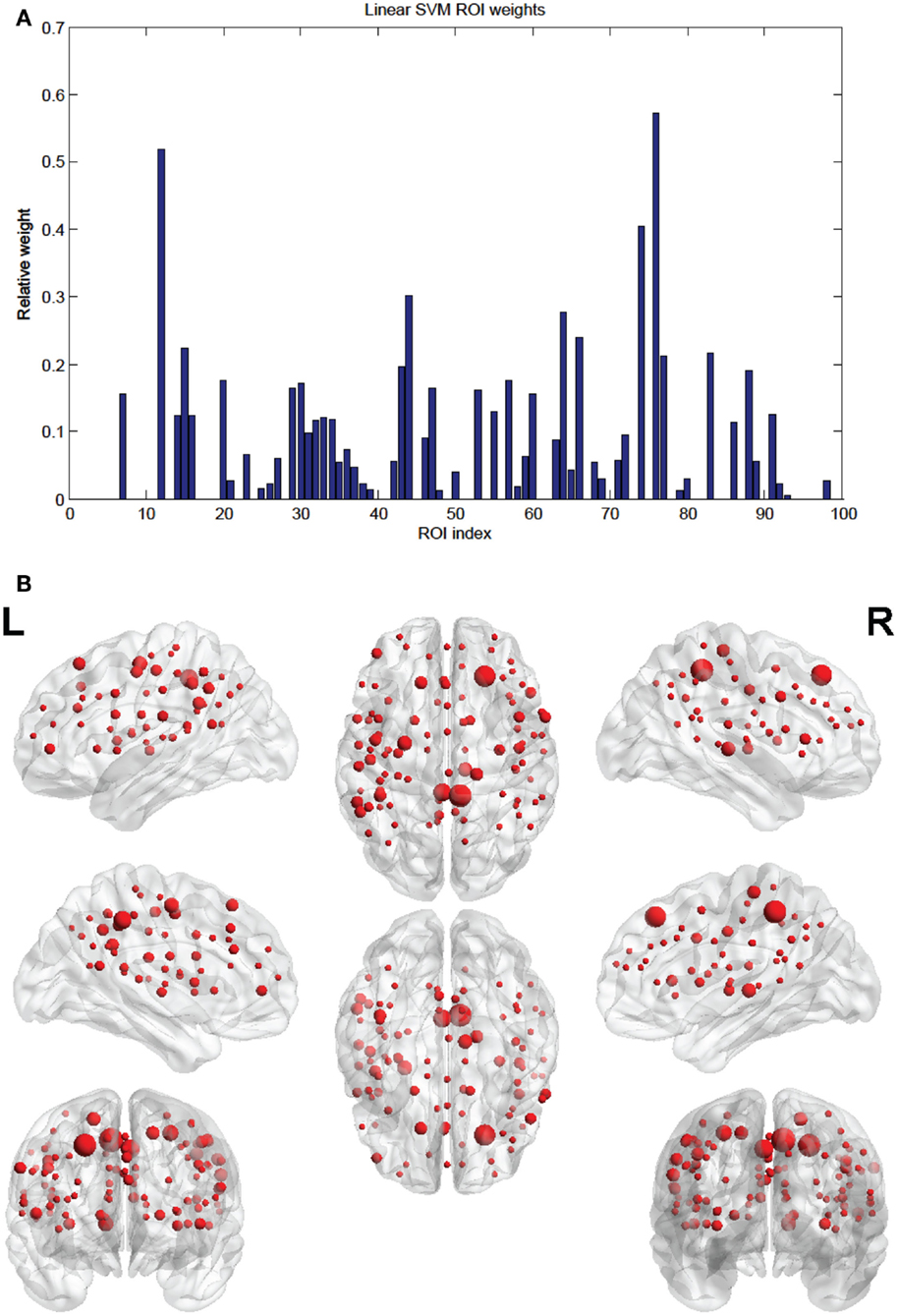
Figure 5. (A) Shows a bar graph representation of the relative weight or contribution of each node to the classifier. (B) Shows a representation of the weighted nodes revealing location using BrainNet Viewer software. Each node’s size is proportional to its weight.
We employed the same SVM method on gender classification as we did for age classification. A linear SVM classifier was not able to significantly discriminate between male and female subjects (55% accuracy, p-value < 0.17, binomial test; compared to 50% for random chance). Also a multi-class linear kernel SVM classifier was applied to 65 subjects partitioned into three age groups: young, middle, and old. It was able to significantly discriminate between the three groups using a linear SVM with 28 top features retained and C = 0.1 (57% accuracy; p-value < 1 × 10⁻⁴, binomial test; compared to ∼33% for random chance).
SVR
Seeing that classification of age groups was successful, we decided to test whether age prediction of individuals is viable on a continuous scale with the use of only fcMRI data. That is, given an fMRI connectivity map, we wanted to determine the age in years of the individual on a continuous range rather than choose between two or three discrete classes. A SVR linear predictor (top features retained = 298, ε = 0.1) was applied to 65 subjects varying in age (19–85 years) and was able to predict subject age with a reasonable degree of accuracy, [, p-value < 1 × 10⁻⁸ (null hypothesis of no correlation or a slope of zero)], where is a linear regression line applied to the (x, y) points with x being the true age of the subject and y the predicted age (see Figure 6). A similar holdout set method was employed for the SVR predictor as was for the SVM classifiers (see Figures 7 and 8).
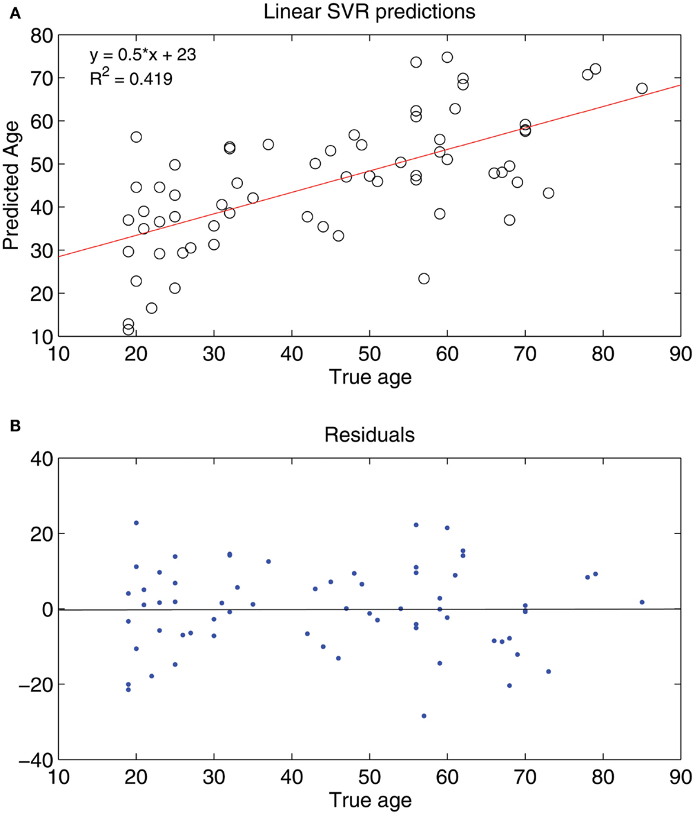
Figure 6. (A) Shows a least squares regression line on the predicted and actual age points. (B) Shows the residuals for the least squares regression fit.
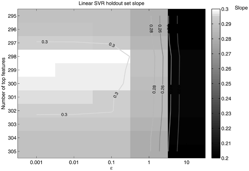
Figure 7. Slope as a function of ε and the number of top features retained. The slope peaks at 298 features retained and ε = 0.1.
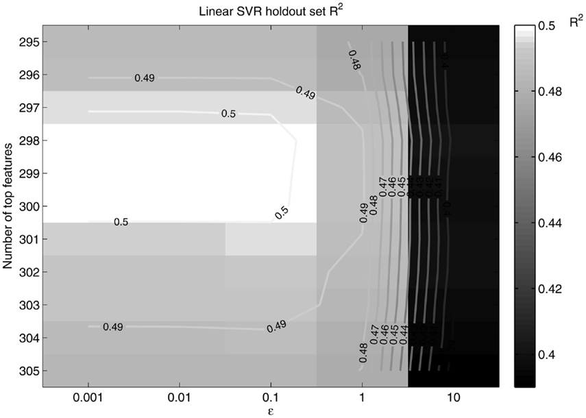
Figure 8. R2 as a function of ε and the number of top features retained. R2 peaks at around 298 features retained and ε = 0.1, in the same neighborhood as the peak slope.
The SVR method had 185 features (out of the 298) present in every fold. These consensus features’ weights and the node weights were computed in the same way as for the SVM classifier (see Figures 9 and 10; Tables 4 and 5).
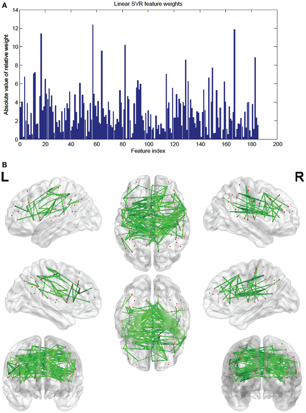
Figure 9. (A) Shows a bar graph representation of the relative weight or contribution of each of the 185 consensus features to the linear kernel SVR predictor. (B) Shows a representation of the 185 consensus features revealing location. Each connection thickness is proportional to the feature weight.
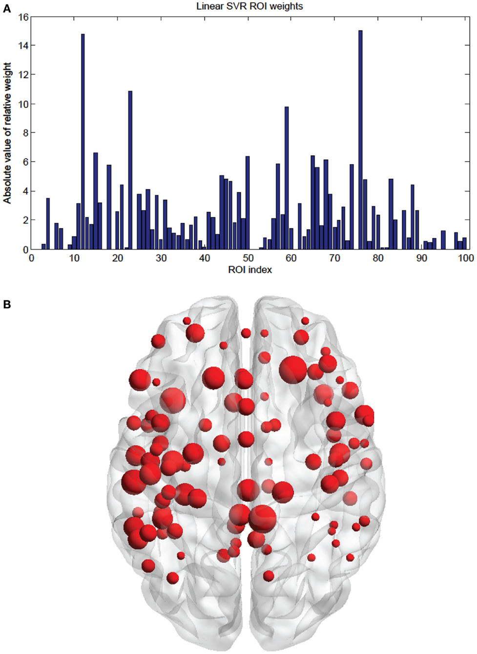
Figure 10. (A) Shows a bar graph representation of the relative weight or contribution of each node to the linear kernel SVR predictor, with ε fixed at 0.1. (B) Shows a representation of the 100 weighted nodes revealing location. Each node’s size is proportional to its weight.
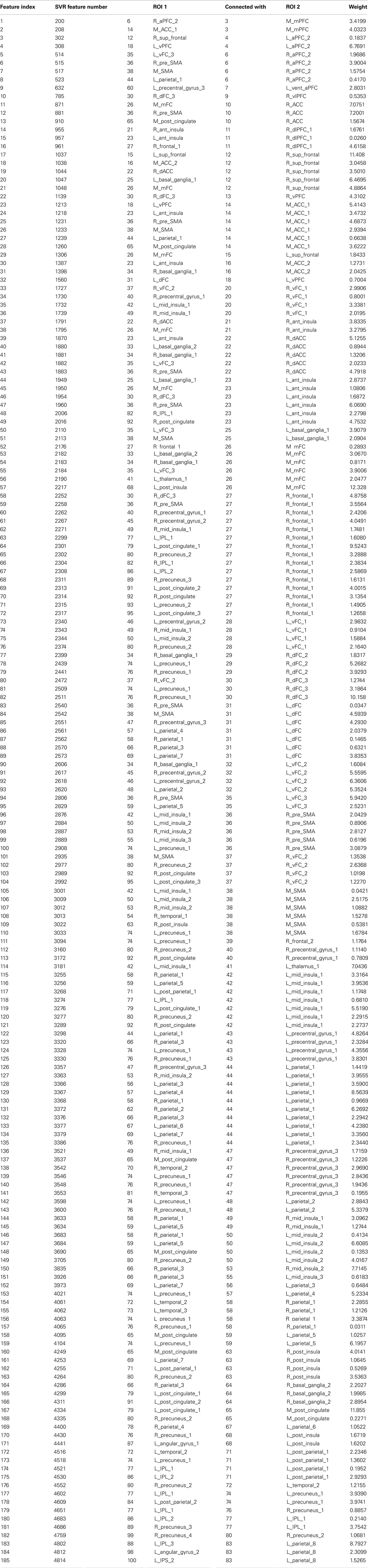
Table 4. A list of the consensus features and their weights for the linear SVR age predictor.

Table 5. Nodes and their weights for the linear kernel SVR predictor.
To check for agreement with previous studies (see Dosenbach et al., 2010), a SVR predictor using a RBF kernel was applied to our same 65 subject data set. The RBF SVR predictor (top features retained = 15, ε = 0.1) was able to predict age comparable to, but worse than, the linear SVR predictor [RBF SVR: R2 = 0.188, p-value < 1 × 10⁻³, (null hypothesis of no correlation or zero slope)]. The node weights were computed in the same way as for the linear SVR case (see Figure 11), and the highest weight nodes are listed in Table 6.
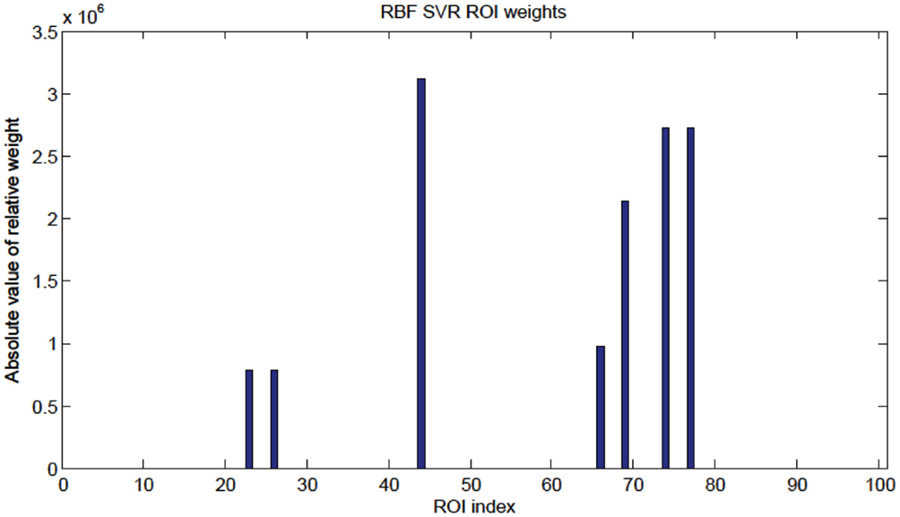
Figure 11. Radial basis function kernel SVR node weights. Since the RBF SVR method used 15 top features total, only seven nodes were present as shown in Table 6.
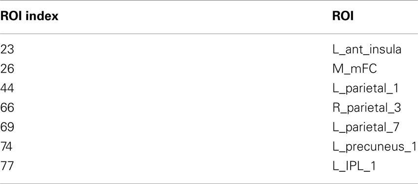
Table 6. Nodes for the RBF SVR predictor.
However, we use the linear SVR predictor for feature and node significance output since weights extracted from the linear SVR have a direct proportionality between absolute weight and significance in variable prediction. The same cannot be said about the RBF SVR weights, which are not as readily interpreted.
Discussion
In the present study, we examined the ability of a SVM to classify individuals as either young or old, and to predict age solely on their rs-fMRI data. Our aim was to improve the discriminatory ability and accuracy of the multivariate vector machine method by parameter tuning and feature selection and also output interpretable discriminating features.
Support vector machine classification (using temporal correlations between ROIs as input features) of individuals as either children or adults was found 91% accurate in a study by Dosenbach et al. (2010), and our 84% accurate age classifier is in agreement with these results. This shows that a SVM classifier can be successfully applied to rs-fMRI functional connectivity data with appropriate feature selection and parameter tuning. Our linear SVM classifier’s performance was comparable to that of the RBF SVM, and only slightly more accurate. One advantage of the linear SVM classifier over the RBF classifier, used by Dosenbach et al. (2010) for feature interpretation, is that the weights extracted from the linear classifier have a direct relationship between absolute weight and the classifier contribution. The RBF classifier weights are more difficult to interpret.
Although age classification was very significant (p-value < 1 × 10⁻⁷), gender classification (p-value < 0.17) was not. This could be due to the lack of significant differences between resting male and female functional connectivity. A recent study by Weissman-Fogel et al. (2010) found no significant differences between genders in resting functional connectivity of the brain areas within the executive control, salient, and the default mode networks. The performance of our classifier is consistent with this result and suggests that functional connectivity may not be significantly different between genders. This also provides confirmation that the SVM method classification is specific to aging and not other characteristics in this group of individuals such as gender.
We found that the SVM method predicted subject age on a continuous scale with relatively good performance. A perfect predictor has a linear regression fit of that is, for a given age, x, the SVR prediction, y, matches that age exactly, implying a fit with R2 = 1. The closer the slope of the regression line approached one, and the closer the R2 value approached one, the better the performance of the predictor was considered to be. The R2 value is a measure of the proportion of variability of the response variable (predicted age) that is accounted for by the independent variable (true age), so an R2 of 0.419 (linear SVR) reveals that a substantial portion of the variability in the predicted age is accounted for by the subject age.
From the linear regression plot (Figure 6) it appears that the younger subjects are overestimated in their predicted age and the older subjects are underestimated in their predicted age. The subjects around age 40–50 are estimated accurately. For this regression fit (the predicted age) ranges from around 30 (when x = 20) to around 80 (when x = 90) so the predicted age range is smaller than the actual age range – this occurrence may be due to similar connectivity maps of ages in a small range (age 25–30 for example). This difficulty in accurately distinguishing subjects within a small age range could suggest non-significant age-related inter-subject differences in functional connectivity of subjects in small adult age ranges.
The SVM method allows for detection of the most influential features and nodes which drive the classifier or predictor. We utilized this approach to find the “connectivity hubs,” or nodes with the most significant features that influenced age classification. Tables 3 and 5 reveal the 10 most influential nodes for the linear age SVM classifier and for the linear SVR predictor, respectively. Four out of the 10 most influential nodes are present in both methods: R_precuneus_1, R_sup_frontal, L_precuneus_1, and L_sup_frontal (see Figures 12 and 13). There is a similar degree of agreement between the RBF SVR nodes and the linear SVR nodes: L_precuneus_1, L_parietal_1, R_parietal_3, and L_IPL_1 are in both methods. This agreement between classifier and predictor methods suggests that the connectivity of these nodes provides discriminatory information with respect to age differences with some independence of choice of method.
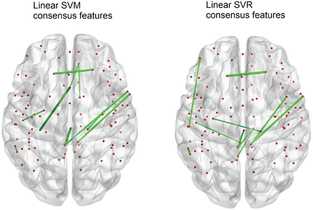
Figure 12. A comparison of the 10 top consensus features for SVM and SVR. Each connection thickness is proportional to the feature weight. Overlap of features indicates an agreement for both age classification and prediction techniques.

Figure 13. A comparison of the 10 top nodes for SVM and SVR. Each node size is proportional to the feature weight. Overlap of nodes indicates an agreement for both age classification and prediction techniques.
Of note is the difference in distributions of the node weights for the linear SVM and linear SVR methods (Figures 5 and 10). The SVM result seems to have only a few high valued nodes with many quite small valued ones, indicating a more abrupt distribution. The SVR node weight values are distributed more uniformly, with high valued nodes, middle valued, and low valued ones occurring frequently. This could be attributed to the difference in the number of top features retained by the two methods. Since features were projected into their respective nodes and the SVM had 100 features retained while the SVR had 298, the distribution of the SVR node values seemed more uniform.
The improvement in accuracy due to the reduction of the dimension of the feature space, in general, reveals that the classification performance is related to the number of features used and the “quality” of the features used. Our work, using the t-test feature filter method for SVM and the correlation feature filter method for SVR as well as the method for parameter selection, shows that SVM classifiers and SVR predictors can achieve high degrees of performance.
The growing number of imaging-based binary classification studies of clinical populations (autism, schizophrenia, depression, and attention-deficit hyperactivity disorder) suggests that this is a promising approach for distinguishing disease states from healthy brains on the basis of measurable differences in spontaneous activity (Shen et al., 2010; Zhang and Raichle, 2010). In addition, several recent studies have demonstrated that the rs-fMRI measurements are reproducible and reliable in young and old populations (Shehzad et al., 2009; Thomason et al., 2011; Song et al., 2012) so a brief resting MRI scan could provide valuable information to aid in screening, diagnosis, and prognosis of patients (Saur et al., 2010). Our own work supports the results that rs-fMRI data contain enough information to make multivariate classifications and predictions of subjects. As the amount of available rs-fMRI data increases, multivariate pattern analysis methods will be able to extract more meaningful information which can be used in complement with human clinical diagnoses to improve overall efficacy.
Conflict of Interest Statement
The authors declare that the research was conducted in the absence of any commercial or financial relationships that could be construed as a potential conflict of interest.
Acknowledgments
This work was supported by the National Research Service Award (NRSA) T32 EB011434 to Svyatoslav Vergun, University of Wisconsin Institute for Clinical and Translational Research National Institutes of Health (UW ICTR NIH)/UL1RR025011 Pilot Grant from the Clinical and Translational Science Award (CTSA) program of the National Center for Research Resources (NCRR) and KL2 Scholar Award to Vivek Prabhakaran, and RC1MH090912 National Institutes of Health-National Institute of Mental Health (NIH-NIMH) ARRA Challenge Grant to Elizabeth Meyerand. We are thankful to the 1000 Functional Connectome Project for their data set.
Footnotes
References
Ben-Hur, A., and Weston, J. (2010). A user’s guide to support vector machines. Methods Mol. Biol. 609, 223–239.
Biswal, B. B., Mennes, M., Zuo, X., Gohel, S., Kelly, C., Smith, S. M., et al. (2010). Toward discovery science of human brain function. Proc. Natl. Acad. Sci. U.S.A. 107, 4734–4739.
Biswal, B. B., Yetkin, F. Z., Haughton, V. M., and Hyde, J. S. (1995). Functional connectivity in the motor cortex of resting human brain using echo-planar MRI. Magn. Reson. Med. 34, 537–541.
Cohen, J. R., Asarnow, R. F., Sabb, F. W., Bilder, R. M., Bookheimer, S. Y., Knowlton, B. J., et al. (2011). Decoding continuous variables from neuroimaging data: basic and clinical applications. Front. Hum. Neurosci. 5:75. doi:10.3389/fnins.2011.00075
Craddock, R. C., Holtzheimer, P. E., Hu, X. P., and Mayberg, H. S. (2009). Disease state prediction from resting state functional connectivity. Magn. Reson. Med. 62, 1619–1628.
Damoiseaux, J. S., Rombouts, S. A. R. B., Barkhof, F., Scheltens, P., Stam, C. J., Smith, S. M., et al. (2006). Consistent resting-state networks across healthy subjects. Proc. Natl. Acad. Sci. U.S.A. 103, 13848–13853.
Dosenbach, N. U., Nardos, B., Cohen, A. L., Fair, D. A., Power, J. D., Church, J. A., et al. (2010). Prediction of individual brain maturity using fMRI. Science 329, 1358–1361.
Drucker, H., Burges, C. J. C., Kaufman, L., Smola, A., and Vapnik, V. N. (1997). “Support vector regression machines” in Advances in Neural Information Processing Systems, Vol. 9, eds M. C. Mozer, J. Jordan, and T. Petsche (Cambridge, MA: MIT Press), 155–161.
Hastie, T., Tibshirani, R., and Friedman, J. H. (2001). The Elements of Statistical Learning: Data Mining, Inference, and Prediction. New York, NY: Springer Publishing Company, Inc., 193–224.
Haynes, J., and Rees, G. (2005). Predicting the stream of consciousness from activity in human visual cortex. Curr. Biol. 15, 1301–1307.
Hsu, C.-W., Chang, C.-C., and Lin, C.-J. (2010). A Practical Guide to Support Vector Classification. Available at: http://www.csie.ntu.edu.tw/~cjlin/ [accessed January 2012].
Johnson, J. D., McDuff, S. G. R., Rugg, M. D., and Norman, K. A. (2009). Recollection, familiarity, and cortical reinstatement: a multivoxel pattern analysis. Neuron 63, 697–708.
LaConte, S. M., Peltier, S. J., and Hu, X. P. (2007). Real-time fMRI using brain-state classification. Hum. Brain Mapp. 28, 1033–1044.
Meier, T. B., Desphande, A. S., Vergun, S., Nair, V. A., Song, J., Biswal, B. B., et al. (2012). Support vector machine classification and characterization of age-related reorganization of functional brain networks. Neuroimage, 60, 601–613.
Mitchell, T. M., Shinkareva, S. V., Carlson, A., Chang, K., Malave, V. L., Mason, R. A., et al. (2008). Predicting human brain activity associated with the meanings of nouns. Science 320, 1191–1195.
Neuroimaging Informatics Tools and Resources Clearinghouse (NITRC). (2011). Available at: http://www.nitrc.org/frs/?group_id=296 [accessed December 2011].
Norman, K. A., Polyn, S. M., Detre1, G. J., and Haxby, J. V. (2006). Beyond mind-reading: multi-voxel pattern analysis of fMRI data. Trends Cogn. Sci. (Regul. Ed.) 10, 424–430.
Pereira, F., Mitchell, T., and Botvinick, M. (2009). Machine learning classifiers and fMRI: a tutorial overview. Neuroimage 45, S199–S209.
Poldrack, R. A., Halchenko, Y. O., and Hanson, S. J. (2009). Decoding the large-scale structure of brain function by classifying mental states across individuals. Psychol. Sci. 20, 1364–1372.
Saur, D., Ronneberger, O., Kümmerer, D., Mader, I., Weiller, C., and Klöppel, S. (2010). Early functional magnetic resonance imaging activations predict language outcome after stroke. Brain 133, 1252–1264.
Schölkopf, B., and Smola, A. J. (2002). Learning with Kernels: Support Vector Machines, Regularization, Optimization and Beyond. Cambridge, MA: MIT Press, 633.
Schölkopf, B., Tsuda, K., and Vert, J. P. (eds). (2004). Kernel Methods in Computational Biology Computational Molecular Biology. Cambridge: MIT Press.
Schurger, A., Pereira, F., Treisman, A., and Cohen, J. D. (2010). Reproducibility distinguishes conscious from nonconscious neural representations. Science 327, 97–99.
Shehzad, Z., Kelly, A. M. C., Reiss, P. T., Gee, D. G., Gotimer, K., Uddin, L. Q., et al. (2009). The resting brain: unconstrained yet reliable. Cereb. Cortex 19, 2209–2229.
Shen, H., Wang, L., Liu, Y., and Hu, D. (2010). Discriminative analysis of resting-state functional connectivity patterns of schizophrenia using low dimensional embedding of fMRI. Neuroimage 49, 3110–3121.
Smith, S. M., Jenkinson, M., Woolrich, M. W., Beckmann, C. F., Behrens, T. E. J., Johansen-Berg, H., et al. (2004). Advances in functional and structural MR image analysis and implementation as FSL. Neuroimage 23, S208–S219.
Song, J., Desphande, A. S., Meier, T. B., Tudorascu, D. L., Vergun, S., Nair, V. A., et al. (2012). Age-related differences in test-retest reliability in resting-state brain functional connectivity. PLoS ONE 7:e49847. doi:10.1371/journal.pone.0049847
Soon, C., Brass, M., Heinze, H., and Haynes, J. (2008). Unconscious determinants of free decisions in the human brain. Nat. Neurosci. 11, 543–545.
Supekar, K., Musen, M., and Menon, V. (2009). Development of large-scale functional brain networks in children. PLoS. Biol. 7:e1000157. doi:10.1371/journal.pbio.1000157.
Thomason, M. E., Dennis, E. L., Joshi, A. A., Joshi, S. H., Dinov, I. D., Chang, C., et al. (2011). Resting-state fMRI can reliably map neural networks in children. Neuroimage 55, 165–175.
Van Dijk, K. R. A., Hedden, T., Venkataraman, A., Evans, K. C., Lazar, S. W., and Buckner, R. L. (2010). Intrinsic connectivity as a tool for human connectomics: theory, properties, and optimization. J. Neurophysiol. 103, 297–321.
Weissman-Fogel, I., Moayedi, M., Taylor, K. S., Pope, G., and Davis, K. D. (2010). Cognitive and default-mode resting state networks: do male and female brains “rest” differently? Hum. Brain Mapp. 31, 1713–1726.
Weston, J., Elisseeff, A., Bakir, G., and Sinz, F. (2005). The Spider Machine Learning Toolbox. Resource object oriented environment. Available at: http://people.kyb.tuebingen.mpg.de/spider/main.html [accessed December 2011].
Weston, J., and Watkins, C. (1998). Multi-Class Support Vector Machines. Technical Report CSD-TR-98-04, Egham: Department of Computer Science, University of London.
Zhang, D., and Raichle, M. E. (2010). Disease and the brain’s dark energy. Nat. Rev. Neurol. 6, 15–28.
Keywords: aging, resting state fMRI, support vector machine, reorganization
Citation: Vergun S, Deshpande AS, Meier TB, Song J, Tudorascu DL, Nair VA, Singh V, Biswal BB, Meyerand ME, Birn RM and Prabhakaran V (2013) Characterizing functional connectivity differences in aging adults using machine learning on resting state fMRI data. Front. Comput. Neurosci. 7:38. doi: 10.3389/fncom.2013.00038
Received: 17 July 2012; Accepted: 02 April 2013;
Published online: 25 April 2013.
Edited by:
Misha Tsodyks, Weizmann Institute of Science, IsraelReviewed by:
Meng Hu, Drexel University, USAAbdelmalik Moujahid, University of the Basque Country, Spain
Copyright: © 2013 Vergun, Deshpande, Meier, Song, Tudorascu, Nair, Singh, Biswal, Meyerand, Birn and Prabhakaran. This is an open-access article distributed under the terms of the Creative Commons Attribution License, which permits use, distribution and reproduction in other forums, provided the original authors and source are credited and subject to any copyright notices concerning any third-party graphics etc.
*Correspondence: Svyatoslav Vergun, Medical Physics, University of Wisconsin–Madison, 1122-Q2 Wisconsin Institutes for Medical Research, 1111 Highland Avenue, Madison, WI 53705, USA. e-mail: svergun@wisc.edu