Variation in Riverine Inputs Affect Dissolved Organic Matter Characteristics throughout the Estuarine Gradient

Introduction

Organic matter (OM) in aquatic systems originates from two distinct sources; autochthonous OM from within the system and allochthonous OM from outside of the system, which in most cases is from terrestrial sources (Peterson et al., 1994). Autochthonous OM dominates in systems with low terrestrial influence, or systems with high nutrient loadings that stimulate high primary production (e.g., eutrophic lakes and coastal areas). Allochthonous OM dominates in systems where there is significant terrestrial influence and moderate nutrient loadings limiting the growth of aquatic primary producers. Most of the aquatic organic matter is in dissolved form (dissolved organic matter; DOM). The DOM pool is highly heterogeneous, and the quality of DOM may vary significantly regardless of quantity. The quality of DOM determines its cycling, bioavailability and reactivity in the environment, i.e., the fate of terrestrial DOM in coastal systems.

During the transport along the hydrological path from a terrestrial source to the open sea, terrestrially-derived DOM is transformed and removed from the water column by various processes. These processes include salt-induced flocculation (Sholkovitz, 1976; Forsgren et al., 1996; Asmala et al., 2014), photo mineralization (Moran and Zepp, 1997; Aarnos et al., 2012), and microbial uptake and degradation (Raymond and Bauer, 2000; Kirchman et al., 2004). These processes may remineralize DOM compounds partially or completely, incorporate organic material in biomass or cause sedimentation of aggregated DOM molecules; effectively changing and decreasing the DOM pool. However, the DOM pool is replenished by autochthonous production in the estuarine environment, for example by exudates from phytoplankton and macro-vegetation (Brylinsky, 1977; Wiebe and Smith, 1977; Romera-Castillo et al., 2010). All these processes combine so that the DOM pool is gradually changing from terrestrial to marine DOM (Koch et al., 2005). In general, there is a continuum from more reactive terrestrial (“young”) DOM to less reactive marine (“old”) DOM, which accumulates in the ocean interior (Jiao et al., 2010).

The quality of the highly heterogeneous DOM pool can be analyzed with multiple analytical approaches (Leenheer and Croué, 2003; Sulzberger and Durisch-Kaiser, 2009; Nebbioso and Piccolo, 2013). Individual quality parameters of bulk DOM have been linked to the chemical properties or biogeochemical reactivity, and these proxies have been widely used in aquatic biogeochemistry. For instance, the spectral slope of colored DOM (CDOM) absorption between wavelengths 275 and 295 nm is a good proxy for the average molecular size of the DOM pool (Helms et al., 2008). Molecular size in turn has been linked to the bioavailability and reactivity of DOM (Tranvik, 1990; Amon and Benner, 1996). Stable carbon isotope ratios of dissolved organic carbon (DOC) can be linked to its origin, as the signal from terrestrial and aquatic primary producers can be differentiated (Peterson et al., 1994; McCallister et al., 2004). DOC-specific absorbance in UV wavelengths (CDOM absorption) and visible light emission from UV excitation (CDOM fluorescence) indicate humic-like properties of the bulk DOM (Coble, 1996; Weishaar et al., 2003).

The role of freshwater residence time in the estuarine studies has been studied, especially in relation to nutrient retention processes (Borum, 1996; Josefson and Rasmussen, 2000; McGlathery et al., 2007). Increasing residence time in estuaries typically increases the biological processing of nutrients, and thus decreases the amount of nutrients reaching the open sea (Church, 1986). However, biological processes within an estuary can transform, decrease or increase DOM along the salinity gradient. The effect of residence time on DOM transformation is not well known. Traditionally, the extent to which biogeochemical processes alter the DOM pool along the estuarine salinity gradient has been analyzed by quantifying deviations from conservative mixing (Officer, 1979). Employing this method, the DOM properties of interest (e.g., DOC concentration) for two salinity end-members of the system are connected with a mixing line and DOM characteristics for intermediate salinities are analyzed to assess if biogeochemical processes, in addition to mixing, significantly affect these observations (Sholkovitz, 1976; Guo et al., 2007; Markager et al., 2011; Asmala et al., 2014). These biogeochemical processes (degradation, production, and transformation of DOM) are all, to some degree, enhanced by increasing residence time.

Even though changes in the DOM pool along estuarine gradients have been studied extensively, most studies have not successfully separated removal, production, and transformation processes from conservative mixing (Mantoura and Woodward, 1983; Abril et al., 2002; Köhler et al., 2003; Bowers et al., 2004; Guo et al., 2007; Spencer et al., 2007a). On the other hand, some studies have been able to show significant non-conservative dynamics in the DOM pool (Uher et al., 2001; Huguet et al., 2009; Markager et al., 2011; Asmala et al., 2014). It is evident that some system- or compound-specific properties determine whether the DOM pool follows conservative mixing in estuaries. As the effect of residence time on DOM dynamics along the estuarine mixing has not been thoroughly studied yet, our objective was to add a new perspective to estuarine changes in DOM, by calculating the freshwater residence time for all our sampling points and analysing its potential influence on DOM properties. Further, our aim was to characterize DOM pool with different analytical approaches and link these to get a synchronized view of the DOM properties along the gradients of salinity and freshwater age. We hypothesize that (1) the freshwater residence time is a valuable predictor of the changes in the DOM pool along the estuarine gradient alongside salinity; (2) changes in the DOM pool are unidirectional and can be measured with different analytical approaches; (3) analysis of the freshwater residence time combined with the multiparametric DOM characterization improves the applicability and accuracy of traditional conservative mixing models.

Materials and Methods

Field Sampling

Our field data comes from transect samplings conducted in three Finnish rivers draining to the Baltic Sea: Karjaanjoki, Kyrönjoki, and Kiiminkijoki, sampled in the spring, summer, and autumn of 2010 and 2011 (Figure 1). Each transect consisted of five to six horizontal sampling points from surface layer and below the river water lens, typically at 5 or 10 m depth. There were 18 transect datasets with n = 187 observations in total.

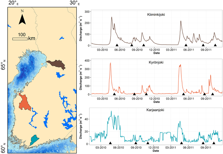
Figure 1. Map of study estuaries and river discharges during the study period. Sampling occasions are marked with a triangle symbol. Catchment of each river is colored with respective color as in discharge graph.

The three catchments have different land-use and consequently the river water properties differ significantly (Asmala et al., 2013, 2014; Kaartokallio et al., in press). Kiiminkijoki and Kyrönjoki have a characteristic spring peak in freshwater runoff due to melting of snow and ice in the catchment, whereas discharges from Karjaanjoki in southern Finland were more evenly distributed over the year (Figure 1). The Karjaanjoki estuary is the longest of the three estuaries with a distance between river and sea end-member of 38 km, and the salinities of the coastal waters were on average 6.3 ± 0.5. In the Kyrönjoki and Kiiminkijoki estuaries the distances between end-members are 36 and 21 km and salinities of the coastal waters were 2.7 ± 1.1 and 2.3 ± 0.1, respectively. Majority of DOM loading in these estuaries originates from the rivers: 15.5% in Karjaanjoki, 0.7% in Kyrönjoki, and 0.0% in Kiiminkijoki (Räike et al., 2012).

In all estuaries surface waters were sampled from the main channels with a small boat or coastal vessel using either a Limnos-type water sampler or polyethylene bucket. The water samples were immediately transferred to 30 L polyethylene canisters, and were stored cool and dark until filtration in laboratory (within 24 h). For analysis of DOM properties, sampled water was filtered through pre-combusted (450°C for 4 h) GF/F (Whatman) filters. Pre-combustion of GF/F filters decrease their nominal pore size so that the effective filtering cut-off is comparable to filters with a nominal pore size of 0.2 μm for freshwater and estuarine bacteria (Nayar and Chou, 2003).

A subset of the filtered samples for colored dissolved organic matter (CDOM) and fluorescent dissolved organic matter (FDOM) were stored in acid-washed, pre-combusted (4h at 450°C) glass vials at 4°C until absorbance and fluorescence measurements were made within 2 weeks from sampling. Filtered DOM samples stored refrigerated have shown negligible changes in both spectral CDOM absorption and humic-like fluorescence characteristics during storage periods of up to 5 months (Boyd and Osburn, 2004; Chen and Gardner, 2004; Retamal et al., 2007; Gueguen et al., 2015). Samples for size-exclusion chromatography (SEC) measurement were stored in acid-washed, pre-combusted glass vials at –20°C until analysis. A subset for DOC analyses were acidified with H₃PO₄ and stored frozen at –20°C until measurement. DOC concentration does not change in filtered and acidified samples when stored frozen for up to 1 year (Benner and Opsahl, 2001; Dittmar et al., 2006; Norman and Thomas, 2014). For stable carbon isotope analysis (δ¹³C_DOC), 500 mL water samples were filtered through pre-combusted GF/F and acidified with HCl to pH 2 to transform all carbonates to CO₂. The acidified samples were frozen and subsequently freeze-dried to attain solid samples.

Analytical Procedures Used

DOC concentrations were analyzed by high temperature combustion on a MQ1000 TOC analyser according to Qian and Mopper (1996). Analysis integrity was tested daily on certified reference material [University of Miami, Consensus Reference Materials, Florida Strait seawater (lot #05–10: 41 to 44 μmol C L⁻¹)]. The method yielded an average DOC concentration of this material of 42 ± 7 (SD) μmol C L⁻¹ (n = 213). Dissolved organic nitrogen (DON) was calculated by subtracting the combined inorganic nitrogen (${\text{NH}}_4^{+}$, ${\text{NO}}_2^{-}$ and ${\text{NO}}_3^{-}$) from the total dissolved nitrogen (TDN; from the filtered fraction). The inorganic nutrient analyses were carried out according to Grasshoff et al. (1983), where the ${\text{NH}}_4^{+}$ analyses were done manually and for the ${\text{NO}}_2^{-}$ and ${\text{NO}}_3^{-}$ analyses an automated flow injection analyser was used (Lachat QC 8000). TDN was determined following alkaline persulfate oxidation (Koroleff et al., 1977; Grasshoff et al., 1999) followed by automated analysis.

Spectrophotometric analyses of CDOM samples were performed using PerkinElmer Lambda 650 UV/VIS spectrophotometer with 1 cm quartz cuvette over the spectral range from 200 to 800 nm with 1 nm intervals. Milli-Q (Millipore) water was used as the reference for all samples. Absorbance measurements were transformed to absorption coefficients by multiplying by 2.303 and dividing by the path length (0.01 m). The spectral slope (S_275−295; μm⁻¹) has been derived from CDOM absorption spectra by fitting the absorption data to the equation: $a_{\lambda }=a_{\lambda \text{ref}}^{e-S(\lambda -\lambda \text{ref})}$ where a = Napierian absorption coefficient (m⁻¹), λ = wavelength (nm), and λ_ref = reference wavelength (nm). The resulting slope coefficient was multiplied by 1000 to convert unit from nm⁻¹ to μm⁻¹. SUVA₂₅₄ values were determined by dividing the UV absorbance measured at 254 nm by the DOC concentration and are reported in the units of square meters per gram carbon.

Excitation/emission matrices of fluorescence were measured for DOM samples in 1 cm quartz cuvette in a Varian Cary Eclipse fluorometer (Agilent). Bandwidths were set to 5 nm for excitation and 4 nm for emission. A series of emission scans (280–600 nm) were collected over excitation wavelengths ranging from 220 to 450 nm by 5 nm increments. Fluorescence spectra were corrected for inner filter effects, which accounted for the absorption of both excitation and emission light by the sample in the cuvette (Mobed et al., 1996). This was done following the methods of Murphy et al. (2010). The fluorescence spectra (excitation and emission) were also corrected for instrument biases using an excitation correction spectrum derived from a concentrated solution of Oxazine 1 and an emission correction spectrum derived using a ground quartz diffuser. Fluorescence spectra were Raman calibrated by normalizing to the area under the Raman scatter peak (excitation wavelength of 350 nm) of a Milli-Q water sample, run on the same session as the samples. To remove the Raman signal, a Raman normalized Milli-Q excitation-emission matrix (EEM) was subtracted from the sample data. As the measured signal was normalized to the Raman peak and excitation and emission correction spectra were used, all the instrument specific biases were effectively removed (Murphy et al., 2010). Rayleigh scatter effects were removed from the data set by not including any emission measurements made at wavelengths = excitation wavelength +20 nm. Most likely due to the high heterogeneity of the samples in relation to number of observations, parallel factor analysis (PARAFAC) was not successful in extracting relevant information from the dataset. Instead, we used the classical peak-picking method, and fluorescence peaks C, A, M, and T were extracted from the EEM data (Coble, 1996). Peak A is a primary fluorescence peak from dissolved humic substances; peak C is a secondary humic substance peak characteristic of terrestrially derived DOM; peak M is a secondary humic substance peak characteristic of microbial DOM; peak T is a peak attributable to fluorescence from the aromatic amino acid tryptophan (Coble, 1996). Being a proxy for humic-like, typically terrestrially derived material, we chose to use only peak A for further analysis.

We analyzed the molecular size of DOM with SEC. The SEC analyser consisted of an integrated autosampler and pump module (GPCmax, Viscotek Corp.), a linear type column [TSK G2000SW_XL column (7.8 × 300 mm, 5 μm particle size, Tosoh Bioscience GmbH)], a guard column (Tosoh Bioscience GmbH) and a UV detector (Waters 486 Tunable Absorbance Detector) set to 254 nm. The flow rate was 0.8 ml min⁻¹ and the injection volume 100 μL. The columns were thermo-regulated in a column oven (Croco-cil 100-040-220P, Cluzeau Info Labo) at 25°C. The data were collected with OmniSEC 4.5 software (Viscotek Corp.). The eluent was 0.01 M acetate buffer at a pH of 7.00 (Vartiainen et al., 1987). Prior to injection, the samples were filtered through a 0.2 μm PTFE syringe filter. The system was calibrated using a combination of standards, as follows: acetone, ethylene glycol, salicylic acid, polystyrene sulphonate (PSS) 3.5 kDa and PSS 6.5 kDa (58, 100, 138, 3610, and 6530 Da, respectively). The calibration curve was linear (R² = 0.99) over the apparent molecular weight (AMW) range tested. Comparison between SEC method and absorbance measurements [a_(CDOM254)] yielded a linear correlation coefficient of 0.92, indicating high qualitative recovery of (C)DOM with the SEC method, as measured from integrated signal from SEC chromatogram. From integrated signal we calculated the weighted average apparent molecular weight (AMW_w).

For stable carbon isotope analysis, acidified and freeze-dried DOM was packed to foil cups and analyzed at the Stable Isotope Facility at UC Davis (USA). There, samples were analyzed for δ¹³C using a PDZ Europa ANCA-GSL elemental analyser interfaced to a PDZ Europa 20-20 isotope ratio mass spectrometer (Sercon Ltd., Cheshire, UK). The resulting carbon delta values are expressed relative to international standard Vienna PeeDee Belemnite. Reported standard deviation for this method is ±0.2‰. δ¹³C was only measured for samples taken in 2011.

Calculation of Freshwater Residence Time

We calculated the freshwater residence time for our surface water samples using measured river discharge, surface salinity, and a volume estimate for each upstream segment to a sampling point, totalling 3 or 4 segments for each of the three river estuaries. This approach can be described as the freshwater transit time, which is the average amount of the water parcel (and its dissolved constituents) spend in the estuary between entrance (river end-member) and exit (sea end-member; Zimmerman, 1976; Sheldon and Alber, 2002). The volume of the upper mixed layer in each segment was determined using the bathymetry and the stratification depth. Area of the polygon bounding each segment was determined using publicly available version of the Google Earth (www.google.com/earth/) service and open Earth Point polygon area tool (http://www.earthpoint.us/) and approximate mean depth using high-resolution nautical maps. The mixed layer depth in each segment was determined from the conductivity-temperature-depth (CTD) profiles taken at each sampling occasion. For one of the spring sampling transects no CTD data was available and corresponding mixed layer depth from previous year's sampling was used.

Using the estimated volume of the upper mixed layer or whole segment, measured surface water salinity at each sampling station and known salinities of seawater and river end-members, a freshwater fraction in each segment was calculated using salinity as a tracer. The freshwater fraction and segment volume were then used to estimate the amount of freshwater in each segment and subsequently the time needed to replace the fresh water in a segment was calculated by using the 10-day average river discharge preceding each sampling occasion. Cumulative age of the freshwater in each segment was calculated by assuming homogeneous mixing and zero lateral exchange between segments, i.e., freshwater in each segment to be completely replaced before entering the next segment downstream the estuary. In estuaries tidal mixing is often limiting the usability of approach described above, however, in the Baltic Sea, tidal variation in water level is virtually absent, allowing us to reliably use this simple estimation.

Statistical Analyses

First, we investigated mixing curves for changes in DOC concentration with salinity to test if end-member concentrations and mixing between these two were constant or varied over time. Linear regressions of DOC versus salinity for each sampling transect (six for each estuary, 18 regressions in total) were fitted, and in contrast to ordinary linear regressions, the residual variation around the regression lines was also allowed to vary with salinity by formulating a linear model for the standard deviation (Carstensen and Weydmann, 2012). Through this modeling approach variations in conservative mixing specific to each transect and potential heteroscedasticity were analyzed for each estuary separately. Due to the low number of observations in each transect, it was not possible to investigate heteroscedasticity for individual transects.

Second, we analyzed if measurements of DOM quality changed consistently with DOC along the estuarine gradients. The investigated DOM quality measurements were SUVA₂₅₄, S_275−295, peak A, δ¹³C_DOC, AMW_W, and the DOC:DON ratios. If these DOM components were processed in the estuaries in a similar way as DOC, relationships between the DOM components and DOC would be linear, whereas significant deviations from linear relationships would indicate that the DOM components were degraded, produced, or transformed at a different rate than DOC along the estuarine gradient. Generalized additive models (GAM) were employed to examine if there were significant departures from linearity in the relationships between DOM quality variables and DOC. The GAM also included a categorical seasonal factor to account for additive differences in the relationships to DOC between spring, summer and autumn transects. If the non-linear component of the GAM was not significant then the relationship was reduced to linearity. Hence, the GAM included two parametric components (slope and seasonal variation) and one non-parametric component (departure from linearity in the DOM quality versus DOC relationship).

Third, we examined interrelationships between DOM quality measurements for the three estuaries separately using a principal component analysis (PCA) for five of the six quality variables. The stable carbon isotope (δ¹³C_DOC) was not included in this analysis, since it was only measured during the second year of sampling. The first two principal components, expressing the most significant changes in the DOM composition, were investigated in relation to salinity, DOC and residence time using GAM.

Finally, we analyzed if the relatively inexpensive DOM quality measurement S_275−295 could be used for predicting other DOM components and if such relationships were uniform across the three estuaries. Further, we were interested in the precision of such relationships. For the general applicability of the approach, parametric models were employed. Exponential relationships for SUVA₂₅₄, peak A, δ¹³C_DOC, AMW_W, and DOC:DON versus S_275−295 were fitted to describe the general curvature in the scatter plots with parameters specific to each estuary. Tests for common intercepts and exponential slopes across the three estuaries were carried out, and the models were reduced when significant differences were not present.

The statistical analyses were carried out in SAS 9.3 using PROC MODEL, PROC GAM, and PROC PRINCOMP.

Results

Relationship between Freshwater Residence Time and Salinity

The calculated freshwater residence time in the studied estuaries varied greatly from 0 days at the river mouth to 395 days in the outer Karjaanjoki estuary. In Kyrönjoki and Kiiminkijoki estuaries the longest residence times were 47 and 13 days, respectively. The relationships between freshwater residence time and salinity were highly variable, as for example freshwater residence time varied from a few days to a few months at salinity around 2 (Figure 2). Freshwater residence time increased sharply at low salinity and gradually flattened toward the seaward end-member. The relationships varied between estuaries and flow regimes: The long and relatively deep Karjaanjoki estuary, which also receives the lowest river discharges, had the highest freshwater residence times in general and the increase of residence time with increasing salinity was the highest in Karjaanjoki estuary. Kyrönjoki and Kiiminkijoki estuaries had higher freshwater discharges, and lower surface volumes, resulting in considerably lower residence times. During seasons with high river flow, the freshwater residence time was generally lower along the salinity gradient as compared to the periods of low river discharge (Figure 2).

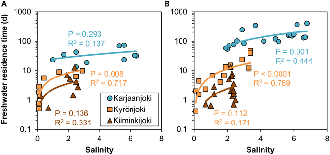
Figure 2. Relationships between freshwater residence time and salinity in the three study estuaries during (A) high (spring) and (B) low (summer and autumn) river discharge conditions. Non-linear power regression models were fitted to data.

Besides freshwater residence time, the quantity and quality of DOM varied between the three estuaries (Table 1). DOM originating from rivers Kiiminkijoki and Kyrönjoki had a higher DOC concentration, more pronounced humic-like signal and relatively larger average molecular size compared to DOM entering the Karjaanjoki estuary. Differences among these estuaries and effects on the DOM characteristics have been discussed in Asmala et al. (2013).

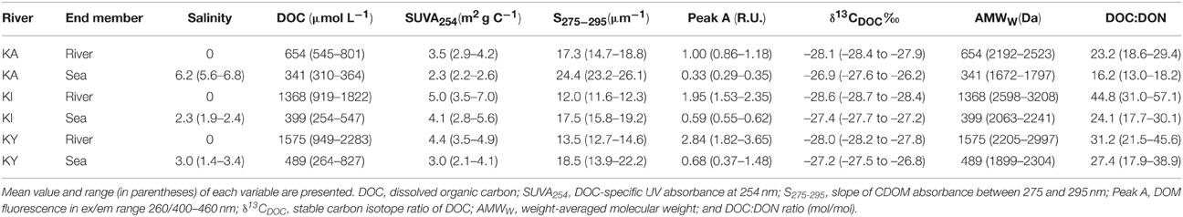
Table 1. Salinity and DOM characteristics for the river and sea end-members in the three studied estuaries (KA = Karjaanjoki, KI = Kiiminjoki, and KY = Kyrönjoki).

Changes in Dom Pool along the Salinity Gradient

In order to analyse the variation of DOM quantity and quality along the estuarine salinity gradient, we modeled the conservative mixing of DOC between the two end-members for each sampling transect separately (Figures 3A–C). There was a considerable variation between the regression lines, particularly for the Kiiminkijoki and Kyrönjoki estuaries, and a pronounced seasonal tendency for mixing of lower DOC concentrations in the two northern estuaries in spring, where freshwater discharge is strongly influenced by snowmelt. Even within seasons the conservative mixing lines varied substantially. Furthermore, we used the residuals from the regression models to quantify the variability of DOC around the mixing line (Figures 3D–F). In essence, the higher the residual the larger is the deviation from conservative mixing. In the Kiiminkijoki and Kyrönjoki estuaries, DOC variability around the mixing line was significantly higher in the freshwater end of the salinity gradient and decreased with increasing salinity, whereas variability around the mixing line was generally smaller in the Karjaanjoki estuary and did not change significantly with salinity.

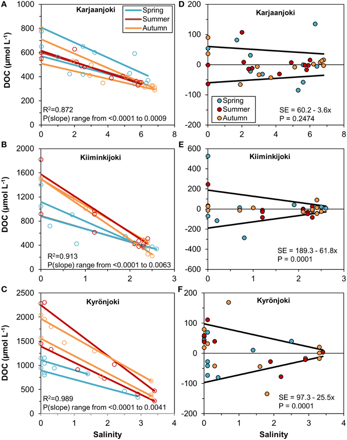
Figure 3. (A–C) Linear regressions between DOC concentration and salinity for each sampling transect, estuary, and season. Observations are shown with open symbols. All slopes are significant (P < 0.05) and the R² is for all regressions within the estuary. (D–F) Residuals from the regression models and the estimated models for the residual standard error for the three estuaries.

We chose six DOM quality variables for this investigation, which are analytically diverse and provide a broad range of the DOM pool properties: Two variables were measured directly with CDOM spectroscopy (S_275−295and fluorescence peak A), one with mass spectrometry (δ¹³C_DOC), and three with combination of analyses (SUVA₂₅₄, AMW_W, DOC:DON). Even though the six variables represent different characteristics and have been measured with different methods, the DOM variables correlated strongly. The selected DOM variables are quality characteristics, and not directly derived from the DOC concentration with the exception of SUVA₂₅₄ and DOC:DON. However, the two latter express ratios between CDOM and DOC, and C and N in the DOM pool and therefore characterize the quality rather than quantity of DOM.

Variable relationships with DOC concentration were observed (Figure 4) and many of them had significant departures from linearity (Table 2). All DOM quality variables had a significant linear GAM component, except for SUVA₂₅₄ in Kiiminkijoki that displayed an oscillating pattern without any clear tendency to change with DOC (Figure 4A). S_275−295had significant non-linear relationships for all three estuaries, decreasing with DOC in an exponential manner (Figure 4B). Peak A had an apparent linear relationship with DOC concentrations below 1000 μmol L⁻¹ with significant departures near the river mouths in Kiiminkijoki and Kyrönjoki estuaries (Figure 4C). On the other hand, the stable carbon isotope signature of DOC (δ¹³C_DOC) changed linearly with DOC throughout the entire scale (Figure 4D). In Kiiminkijoki and Kyrönjoki estuaries changes in AMW_W were small near the river mouths followed by larger, almost linear, declines with DOC (Figure 4E). The DOC:DON ratio increased linearly with DOC in Karjaanjoki and Kiiminkijoki estuaries, whereas the relationship in Kyrönjoki was more complex (Figure 4F). Overall, in Karjaanjoki the DOM quality changed consistently with DOC across the salinity gradient, whereas there were pronounced non-linearities in the relationships with DOC near the freshwater sources in Kiiminkijoki and Kyrönjoki estuaries.

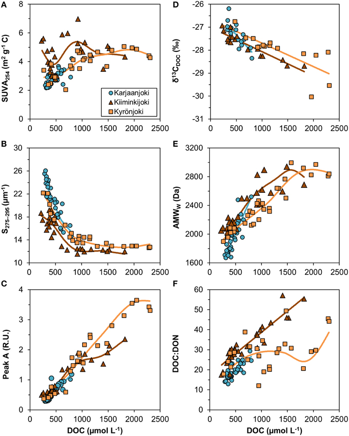
Figure 4. Relationships between DOM quality variables and DOC concentration. (A) SUVA₂₅₄ = DOC-specific UV absorbance at 254 nm, (B) S_275−295 = slope of CDOM absorbance between 275 and 275 nm, (C) peak A = DOM fluorescence in ex/em range 260/400–460 nm, (D) δ¹³C_DOC = stable carbon isotope ratio of DOC, (E) AMW_W = weight-averaged molecular weight, and (F) DOC:DON ratio (mol/mol). Generalized additive models (GAM) are fitted to data (solid lines). The GAM relationships are shown as linear regressions if the non-linear component was not significant (Table 2).

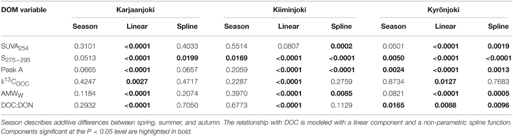
Table 2. Significance of the three GAM components for explaining variations in DOM quality variables in the three estuaries.

In addition to the changes with DOC, there were weak seasonal patterns in the DOM quality variables, except in Kyrönjoki where spring samples generally had higher values of S_275−295 and Peak A, and lower DOC:DON values (Table 2; Figure S1). However, the other DOM quality variables did not show any significant seasonal pattern in Kyrönjoki estuary.

The five DOM quality variables in the PCA were strongly inter-correlated, and the first principal component (PC1) explained between 71 and 82% of variation across the three estuaries (Figure 5). PC1 represented a weighted average of the five DOM quality variables with almost equal weight to each of them, except for DOC:DON in Kyrönjoki estuary that had a slightly lower weight. The second principal component (PC2) explained 10% of the variation in Karjaanjoki, whereas it was more important in the two other estuaries accounting for 20–22% of variation. In all three estuaries, the second component represented a difference between DOC:DON and SUVA₂₅₄.

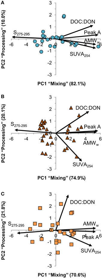
Figure 5. Principal component analysis (PCA) correlation biplot of the two first principal components (PC1 and PC2). Samples are shown as symbols and the contribution of the DOM quality variables to the principal components as vectors. The proportion of variation explained by both principal components is included with the axes titles. (A) Karjaanjoki, (B) Kiiminkijoki, and (C) Kyrönjoki estuary.

We examined the information contained in PC1 and PC2 in relation to salinity, DOC concentration and freshwater residence time (Figure 6). PC1 had a strong, mostly linear relationship with both salinity and DOC concentration (Figures 6A,B), whereas the relationship between PC1 and freshwater residence time was non-linear (Figure 6C). The strongest relationships for PC1 were salinity in Karjaanjoki and DOC in Kiiminkijoki and Kyrönjoki. PC2 was related neither to salinity nor freshwater residence time (Figures 6D,F), whereas a weak coupling to DOC was observed in Kiiminkijoki (Figure 6E). Nevertheless, no general pattern was found using salinity, DOC and freshwater residence time as explanatory variables for the variations in PC2. We have labeled PC1 as “Mixing” and PC2 as “Processing” for clarity, and the justification of this is presented in Section Discussion.

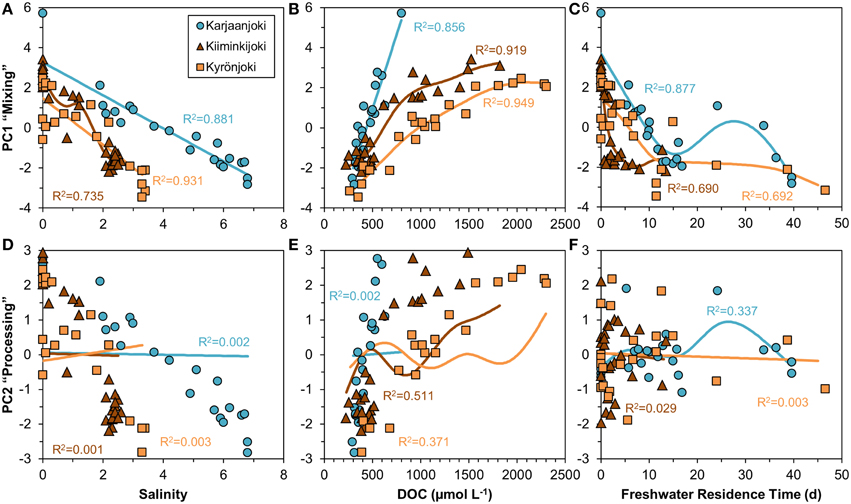
Figure 6. Relationships of the two first principal components versus salinity, DOC concentration and freshwater residence time investigated by a non-parametric GAM (solid line). (A–C) Principal component 1 (“Mixing”). (D–F) Principal component 2 (“Processing”). Freshwater residence time in the Karjaanjoki estuary is divided by 10 for the figure to allow comparison with other two estuaries.

S_275−295 could be used as predictor for the other DOM quality variables with a reasonable precision (Figure 7). Although the relationships estimated for the three estuaries were significantly different (either intercepts or exponential slopes or both were different), the nature of the relationships was similar. For all other five DOM variables the relationship to S_275−295 had an exponential form.

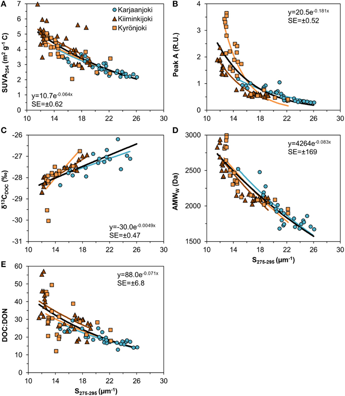
Figure 7. Relationship between UV slope (S_275−295) and other DOM quality variables used in this study. (A) SUVA₂₅₄; (B) Fluorescence peak A; (C) ${}_{\delta }^{13}{\text{C}}_{\text{DOC}}$; (D) AMW_W; (E) DOC:DON ratio. Exponential models were fitted to data for each estuary after testing for common intercepts and exponential slopes. A common model (black line) was fitted to all data with the formula and the residual standard error (SE) inserted in the plots.

Discussion

In order to improve our understanding about the role of DOM processing along the estuarine passage from the river mouth to the open sea, we calculated the residence time for our study estuaries (Figure 2). We observed significant variation in freshwater residence time along the salinity gradient. This variation reveals that at a given salinity on the estuarine gradient the “age” of the freshwater fraction may vary considerably, which has further implications on the associated nutrient and organic matter pool. The calculated freshwater residence time at the sea end-member ranged from 2 to 396 days, depending on the estuary and the flow regime (Table 1). This range covers the reported residence times in different estuarine systems: 0.8–2.7 days (Childs and Quashnet estuaries, USA; Geyer, 1997), 2–210 days (Childs, Columbia, Parker, Satilla and Susquehanna estuaries, USA; Hopkinson et al., 1998), 20–180 days (Choptank and Pocomoke estuaries, USA; Bouvier and del Giorgio, 2002), 4–36 days (Bangpakong estuary, Thailand; Buranapratheprat et al., 2002), and 2–100 days (Fourleague Bay; Perez et al., 2011). Our aim was to use calculated residence time to detect patterns in freshwater dynamics in the estuaries, possibly explaining the variation in DOM quantity and quality.

We were able to identify two distinct freshwater discharge patterns in our dataset; low and high flow conditions. During the low flow, less freshwater enters the estuarine system and the inferred freshwater residence time increases compared to high flow conditions. Essentially, during low flow conditions, freshwater residence time is higher at a given salinity compared to high flow conditions. Low flow conditions occur in summer and autumn, simultaneously with significant autochthonous OM production and high photo-oxidation (Vodacek et al., 1997; Lønborg et al., 2009), potentially changing the DOM pool. To quantify the variation in DOC concentration along the estuarine gradient, we used a linear regression model for each sampling transects separately (Figure 3). Variation in DOC concentration was high in freshwater end-member, from ±60 μmol L⁻¹ in Karjaanjoki to ±190 μmol L⁻¹ in Kiiminkijoki. Variation decreased rapidly when moving along the salinity gradient, reflecting the stability of the coastal sea end-member. This is not surprising, as the freshwater discharge in riverine systems typically fluctuates on seasonal and even diel timescales (Spencer et al., 2007b; Holmes et al., 2012). Most of the DOC in these estuaries originates from the respective river, and not from external point sources (Räike et al., 2012). So it can be argued that the changes in DOM characteristics are in major part due to the alterations of the initial DOM entering the estuary (as opposed to being an artifact of DOM additions within the estuary). Further, in the catchment area different biological processes and human activities cause changes in hydrological conditions and organic matter fluxes from the terrestrial system (Jickells, 1998; Sachse et al., 2005; Asmala et al., 2013). Thus, the combination of changes in discharge and changes in organic matter loading from catchment create large temporal variations in the DOM pool entering the estuaries.

We observed that different DOM quality variables changed differently in relation to DOC concentration (Figure 4). For instance, the stable carbon isotope signature of DOC and humic-like fluorescence had almost linear relationships with DOC concentration, meaning that processes changing the quantity of DOM change these quality indices in similar proportion. On the other hand, SUVA₂₅₄ shows no clear pattern along the measured DOC concentration range, whereas both S_275−295 and molecular weight had coherent, non-linear relationships. The patterns of the slopes and the molecular weight versus DOC in Kyrönjoki and Kiiminkijoki estuaries suggests that part of the DOM pool remains unchanged even though the DOC concentration decreases. In other words, there are components in the DOM pool that persist after the first phases of the degradation processes in the estuarine transport, such as flocculation and microbial degradation.

The analyzed DOM quality characteristics were highly correlated (Figure 5), even though different analytical methods to characterize DOM were used. We argue that the observed high correlation between different quality parameters of the bulk DOM is an indication that common transformations have occurred along the salinity gradients. Also, the changes along the salinity gradient were unidirectional with the expected changes according to the reactivity continuum concept (Amon and Benner, 1996). Our results suggest, that mixing and processing together cause molecules in the DOM pool to decrease in size, lose aromaticity and have a lighter carbon isotope composition when moving down the reactivity (salinity) continuum. PCA was used to examine the relationships between the DOM quality variables (Figure 5). Further, we compared the results of PCA to salinity, DOC concentration and freshwater residence time for a better understanding of DOM processing during the estuarine transport (Figure 6). From the strong correlation between the first principal component (PC1) and both salinity and DOC concentration (Figures 6A,B), it is evident that PC1 actually describes mixing of the two end-members, and is labeled in Results Section accordingly. The second principal component (PC2) on the other hand, does not correlate with salinity, DOC concentration or freshwater residence time, indicating some DOM transformation processes not explained by mixing, DOC concentration or residence time. PC2 was labeled as processing to cover all changes in DOM properties that cannot be attributed to mixing. The weak link between PC2 (processing) and DOC concentration suggests that changes in quantity and quality of DOM are to some extent decoupled.

We used multiple analytical methods in this study to characterize the DOM pool, but still only some components or fractions of the DOM pool were measured, a bias which might have implications when interpreting the results. Specifically, with spectroscopic analyses the non-colored DOM was not detected by most of our methods. This non-colored pool of DOM might be biogeochemically highly relevant, containing such reactive components as amino acids or simple carbohydrates (Vodacek et al., 1997; Sulzberger and Durisch-Kaiser, 2009). The selectivity of DOM analyses is ubiquitous; virtually all methods used to characterize DOM leave parts of the whole pool undetected. From an analytical perspective, the UV absorption slope (S_275−295) proved to be a useful predictor for other DOM variables (Figure 7). The applicability of this slope has been shown in previous studies (e.g., Helms et al., 2008; Fichot and Benner, 2012), and because of its relatively easy and inexpensive analysis, it is highly recommended to continue to use this spectral region as a standard biogeochemical marker in monitoring the DOM-related processes in aquatic environments.

Typically, conservative mixing models have been used to analyse the extent of allochthonous DOM processing in estuarine systems (e.g., Stedmon and Markager, 2003; Boyd and Osburn, 2004). Our data suggests that the variation in DOM quantity and quality occurring in relatively short timescale (days-weeks) poses significant challenges for drawing conclusions from conservative mixing models (Figure 3). The range of the variation in the end-members ultimately determines the applicability of conservative mixing model. Previous studies where non-conservative behavior of DOM has been observed, typically include multiple quantitative and qualitative variables, which show that some parameters deviate from conservative mixing while others do not (Bowers et al., 2004; Markager et al., 2011; Asmala et al., 2014). These qualitative changes can be attributed to simultaneous production and removal of DOM, which may leave the concentration in seemingly steady state, but in fact the DOM pool is subject to continuous dynamic processes.

In this study, we emphasize the importance of taking the variation in freshwater end-member into account in the analysis of DOM processes along the estuarine gradient (Figures 3D–F). Quantification of this variation is especially important when using conservative mixing models to study the DOM transformation, removal and production processes in estuaries, as a relatively large variation on the other end will cause instability throughout the observation range. In coastal systems, the sea end-member is typically relatively stable compared to the freshwater end-member (Fleming-Lehtinen et al., 2014). The results of this study are also supported by long-term time series from the study estuaries, where the measured total organic carbon concentrations range fourfold in Karjaanjoki and Kyrönjoki, and five-fold in Kiiminkijoki (Figure 8). Also, the amount of variation is changing between estuaries, making the predictions about a “typical” situation even more difficult. Without knowledge of the amount and drivers of end-member variations in estuarine studies, analyses based on conservative mixing models will be evidently inadequate as the large variation in the river end-member is carried over throughout the estuarine gradient, thus introducing source of error in conservative mixing models. And as this pattern of variation is evident for DOM quantity, it is highly likely that similar system- and season-specific variations can be observed for DOM quality characteristics as well.

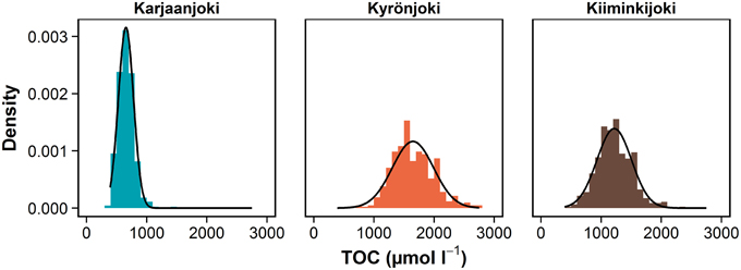
Figure 8. Density of observed TOC concentrations in river end-members of study estuaries between 1975 and 2014. Mean values, standard deviation and range: Karjaanjoki (n = 442) 655 (126, 392–1417), Kyrönjoki (n = 425) 1648(342, 758–2750), and Kiiminkijoki (n = 463) 1217(287, 467–2333) μmol L⁻¹. More than 90% of TOC is in dissolved form (DOC) in these systems (Mattsson et al., 2005). Data source: Räike et al. (2012). Normal distribution curve is fitted over each density histogram.

Residence time in the studied systems is likely not long enough to allow biogeochemical processes to significantly alter the major, refractory part of the DOM pool, especially in the two northernmost estuaries (Figure 2). However, this approach is significantly altered if we do not assume that the terrestrial signal of the DOM pool is refractory, but instead assume that the estuarine DOM pool is being constantly replenished, depleted and transformed. These changes in the DOM pool result as a dynamic state where the balance between various processes determines the resulting characteristics of the bulk DOM. For these particular estuaries, flocculation and bacterial degradation of DOM have been reported (Asmala et al., 2013, 2014), and high rates of photodegradation have been measured in the coastal Baltic Sea (Aarnos et al., 2012). Further, production of DOM by the marine primary producers is evident (Romera-Castillo et al., 2010). Also, heterotrophic bacteria may produce CDOM from non-colored DOM, thus changing the quality of the DOM pool (Nelson et al., 2004; Shimotori et al., 2010). The highly dynamic nature of these processes and the inherent variability in the river end-member pose significant challenges for identification of deviations from conservative mixing in estuaries. In order to analyse the estuarine conservative mixing in a given system, the biogeochemical processes that affect the DOM pool along the estuarine gradient should be identified and quantified, alongside detailed hydrologic measurements.

In conclusion, we surprisingly found that the residence time in these systems did not explain variation any better than salinity. Increasing freshwater residence time in estuaries typically increases the nutrient retention, which can be analyzed with simple mass balance calculations, as production of nutrients within estuary is insignificant compared to the magnitude of nutrient removal processes. With organic matter the biogeochemical cycling is much more complex and dynamic, and transformation, degradation, and production of DOM occur continuously. Our results show that mixing is the major factor governing the characteristics of the DOM pool along the estuarine gradient. Further, we show that variations in DOM pool at the freshwater end-member can introduce substantial departures from linear mixing, but the quality of the DOM pool is not altered consistently with the DOM quantity. Therefore, mixing can only partially account for changes in the DOM pool along the estuarine gradient and more research on the various transformation processes is needed to understand the variability of DOM quality at the land-sea interface.

Author Contributions

EA participated in the experiment design, performed most of the field samplings, conducted most of the laboratory analyses, participated in data analyses and was responsible for the manuscript preparation. HK participated in the experiment design, field samplings, and the laboratory analyses, was responsible for the residence time calculation and participated in manuscript preparation. JC was responsible of principal component analysis and general additive model, and participated in manuscript preparation. DT led the experiment design, and participated field samplings and the laboratory analyses, and participated in manuscript preparation.

Conflict of Interest Statement

The authors declare that the research was conducted in the absence of any commercial or financial relationships that could be construed as a potential conflict of interest.

Acknowledgments

This study was supported by the Academy of Finland (Finland Distinguished Professor Programme, project no. 127097), Walter and Andrée de Nottbeck Foundation and the BONUS COCOA project (grant agreement 2112932-1), funded jointly by the EU and Danish Research Council. The authors would like to thank Riitta Autio, Chris Hulatt, Anne-Mari Luhtanen, and Johanna Oja, for field and laboratory support. Support for sampling was also given by staff from the Tvärminne Zoological Station, South Ostrobothnia and North Ostrobothnia Centres for Economic Development, Transport and the Environment, and Kiviniemi Association of Finnish Lifeboat Institution.

Supplementary Material

The Supplementary Material for this article can be found online at: https://www.frontiersin.org/article/10.3389/fmars.2015.00125

Figure S1. Seasonal patterns of DOM quality predicted for average DOC in the different estuaries (Karjaanjoki 465, Kiiminkijoki 688, and Kyrönjoki 1026 μmol L−1). (A) SUVA₂₅₄; (B) Slope 275–295 nm; (C) Fluorescence peak A; (D) δ13CDOC; (E) AMW_W; (F) DOC:DON ratio. Error bars indicate SE of the seasonal means. Asterisks indicate significance level (cf. Table 2) with *<0.05 and **<0.01.

References

Aarnos, H., Ylöstalo, P., and Vähätalo, A. V. (2012). Seasonal phototransformation of dissolved organic matter to ammonium, dissolved inorganic carbon, and labile substrates supporting bacterial biomass across the Baltic Sea. J. Geophys. Res. Biogeosci. 117:G01004. doi: 10.1029/2010jg001633
Abril, G., Nogueira, M., Etcheber, H., Cabeçadas, G., Lemaire, E., and Brogueira, M. J. (2002). Behaviour of organic carbon in nine contrasting European estuaries. Estuar. Coast. Shelf Sci. 54, 241–262. doi: 10.1006/ecss.2001.0844
Amon, R. M., and Benner, R. (1996). Bacterial utilization of different size classes of dissolved organic matter. Limnol. Oceanogr. 41, 41–51. doi: 10.4319/lo.1996.41.1.0041
Asmala, E., Autio, R., Kaartokallio, H., Pitkänen, L., Stedmon, C., and Thomas, D. N. (2013). Bioavailability of riverine dissolved organic matter in three Baltic Sea estuaries and the effect of catchment land use. Biogeosciences 10, 6969–6986. doi: 10.5194/bg-10-6969-2013
Asmala, E., Bowers, D. G., Autio, R., Kaartokallio, H., and Thomas, D. N. (2014). Qualitative changes of riverine dissolved organic matter at low salinities due to flocculation. J. Geophys. Res. Biogeosci. 119, 1919–1933. doi: 10.1002/2014jg002722
Benner, R., and Opsahl, S. (2001). Molecular indicators of the sources and transformations of dissolved organic matter in the Mississippi river plume. Org. Geochem. 32, 597–611. doi: 10.1016/S0146-6380(00)00197-2
Borum, J. (1996). “Shallow waters and land/sea boundaries,” in Eutrophication in Coastal Marine Ecosystems, eds B. B. Jørgensen and K. Richardson (Washington, DC: American Geophysical Union). doi: 10.1029/CE052p0179
Bouvier, T. C., and del Giorgio, P. A. (2002). Compositional changes in free-living bacterial communities along a salinity gradient in two temperate estuaries. Limnol. Oceanogr. 47, 453–470. doi: 10.4319/lo.2002.47.2.0453
Bowers, D. G., Evans, D., Thomas, D. N., Ellis, K., and Williams, P. L. B. (2004). Interpreting the colour of an estuary. Estuar. Coast. Shelf Sci. 59, 13–20. doi: 10.1016/j.ecss.2003.06.001
Boyd, T. J., and Osburn, C. L. (2004). Changes in CDOM fluorescence from allochthonous and autochthonous sources during tidal mixing and bacterial degradation in two coastal estuaries. Mar. Chem. 89, 189–210. doi: 10.1016/j.marchem.2004.02.012
Brylinsky, M. (1977). Release of dissolved organic matter by some marine macrophytes. Mar. Biol. 39, 213–220. doi: 10.1007/BF00390995
Buranapratheprat, A., Yanagi, T., Boonphakdee, T., and Sawangwong, P. (2002). Seasonal variations in inorganic nutrient budgets of the Bangpakong Estuary, Thailand. J. Oceanogr. 58, 557–564. doi: 10.1023/A:1021214726762
Carstensen, J., and Weydmann, A. (2012). Tipping points in the Arctic: Eyeballing or statistical significance? Ambio 41, 34–43. doi: 10.1007/s13280-011-0223-8
Chen, R. F., and Gardner, G. B. (2004). High-resolution measurements of chromophoric dissolved organic matter in the Mississippi and Atchafalaya River plume regions. Mar. Chem. 89, 103–125. doi: 10.1016/j.marchem.2004.02.026
Church, T. M. (1986). Biogeochemical factors influencing the residence time of microconstituents in a large tidal estuary, Delaware Bay. Mar. Chem. 18, 393–406. doi: 10.1016/0304-4203(86)90020-4
Coble, P. G. (1996). Characterization of marine and terrestrial DOM in seawater using excitation-emission matrix spectroscopy. Mar. Chem. 51, 325–346. doi: 10.1016/0304-4203(95)00062-3
Dittmar, T., Hertkorn, N., Kattner, G., and Lara, R. J. (2006). Mangroves, a major source of dissolved organic carbon to the oceans. Global Biogeochem. Cycles 20:GB1012. doi: 10.1029/2005GB002570
Fichot, C. G., and Benner, R. (2012). The spectral slope coefficient of chromophoric dissolved organic matter (S275–295) as a tracer of terrigenous dissolved organic carbon in river−influenced ocean margins. Limnol. Oceanogr. 57, 1453–1466. doi: 10.4319/lo.2012.57.5.1453
Fleming-Lehtinen, V., Räike, A., Kortelainen, P., Kauppila, P., and Thomas, D. N. (2014). Organic carbon concentration in the northern coastal Baltic Sea between 1975 and 2011. Estuaries Coasts 38, 466–481. doi: 10.1007/s12237-014-9829-y
Forsgren, G., Jansson, M., and Nilsson, P. (1996). Aggregation and sedimentation of iron, phosphorus and organic carbon in experimental mixtures of freshwater and estuarine water. Estuar. Coast. Shelf Sci. 43, 259–268. doi: 10.1006/ecss.1996.0068
Geyer, W. R. (1997). Influence of wind on dynamics and flushing of shallow estuaries. Estuar. Coast. Shelf Sci. 44, 713–722. doi: 10.1006/ecss.1996.0140
Grasshoff, K., Ehrhardt, M., and Kremling, K. (1983). Methods of Seawater Analysis. Weinheim: Verlag Chemie.
Grasshoff, K., Kremling, K., and Ehrhardt, M. (1999). Methods of Seawater Analysis. Weinheim: Verlag Chemie.
Gueguen, C., Itoh, M., Kikuchi, T., Eert, J., and Williams, W. J. (2015). Variability in dissolved organic matter optical properties in surface waters in the Amerasian Basin. Front. Mar. Sci. 2:78. doi: 10.3389/fmars.2015.00078
Guo, W., Stedmon, C. A., Han, Y., Wu, F., Yu, X., and Hu, M. (2007). The conservative and non-conservative behavior of chromophoric dissolved organic matter in Chinese estuarine waters. Mar. Chem. 107, 357–366. doi: 10.1016/j.marchem.2007.03.006
Helms, J. R., Stubbins, A., Ritchie, J. D., Minor, E. C., Kieber, D. J., and Mopper, K. (2008). Absorption spectral slopes and slope ratios as indicators of molecular weight, source, and photobleaching of chromophoric dissolved organic matter. Limnol. Oceanogr. 53, 955. doi: 10.4319/lo.2008.53.3.0955
Holmes, R. M., McClelland, J. W., Peterson, B. J., Tank, S. E., Bulygina, E., Eglinton, T. I., et al. (2012). Seasonal and annual fluxes of nutrients and organic matter from large rivers to the Arctic Ocean and surrounding seas. Estuaries Coasts 35, 369–382. doi: 10.1007/s12237-011-9386-6
Hopkinson, C. S., Buffam, I., Hobbie, J., Vallino, J., Perdue, M., Eversmeyer, B., et al. (1998). Terrestrial inputs of organic matter to coastal ecosystems: an intercomparison of chemical characteristics and bioavailability. Biogeochemistry 43, 211–234. doi: 10.1023/A:1006016030299
Huguet, A., Vacher, L., Relexans, S., Saubusse, S., Froidefond, J. M., and Parlanti, E. (2009). Properties of fluorescent dissolved organic matter in the Gironde Estuary. Org. Geochem. 40, 706–719. doi: 10.1016/j.orggeochem.2009.03.002
Jiao, N., Herndl, G. J., Hansell, D. A., Benner, R., Kattner, G., Wilhelm, S. W., et al. (2010). Microbial production of recalcitrant dissolved organic matter: long-term carbon storage in the global ocean. Nat. Rev. Microbiol. 8, 593–599. doi: 10.1038/nrmicro2386
Josefson, A. B., and Rasmussen, B. (2000). Nutrient retention by benthic macrofaunal biomass of Danish estuaries: importance of nutrient load and residence time. Estuar. Coast. Shelf Sci. 50, 205–216. doi: 10.1006/ecss.1999.0562
Kaartokallio, H., Asmala, E., Autio, R., and Thomas, D. N. (in press). Bacterial production, abundance and cell properties in boreal estuaries: relation to dissolved organic matter quantity and quality. Aquat. Sci. doi: 10.1007/s00027-015-0449-9
Kirchman, D. L., Dittel, A. I., Findlay, S. E., and Fischer, D. (2004). Changes in bacterial activity and community structure in response to dissolved organic matter in the Hudson River, New York. Aquat. Microb. Ecol. 35, 243–257. doi: 10.3354/ame035243
Koch, B. P., Witt, M., Engbrodt, R., Dittmar, T., and Kattner, G. (2005). Molecular formulae of marine and terrigenous dissolved organic matter detected by electrospray ionization Fourier transform ion cyclotron resonance mass spectrometry. Geochim. Cosmochim. Acta 69, 3299–3308. doi: 10.1016/j.gca.2005.02.027
Köhler, H., Meon, B., Gordeev, V. V., Spitzy, A., and Amon, R. M. W. (2003). Dissolved organic matter (DOM) in the estuaries of Ob and Yenisei and the adjacent Kara-Sea, Russia. Proc. Mar. Sci. 6, 281–309.
Koroleff, F., Palmork, K. H., Oe, U., and Gieskes, J. M. (1977). The international Intercalibration Exercise for Nutrient Methods. Cooperative Research Report (Charlottenlund). 67.
Leenheer, J. A., and Croué, J. P. (2003). Peer reviewed: characterizing aquatic dissolved organic matter. Environ. Sci. Technol. 37, 18A–26A. doi: 10.1021/es032333c
Lønborg, C., Davidson, K., Álvarez–Salgado, X. A., and Miller, A. E. (2009). Bioavailability and bacterial degradation rates of dissolved organic matter in a temperate coastal area during an annual cycle. Mar. Chem. 113, 219–226. doi: 10.1016/j.marchem.2009.02.003
Mantoura, R. F. C., and Woodward, E. M. S. (1983). Conservative behaviour of riverine dissolved organic carbon in the Severn Estuary: chemical and geochemical implications. Geochim. Cosmochim. Acta 47, 1293–1309. doi: 10.1016/0016-7037(83)90069-8
Markager, S., Stedmon, C. A., and Søndergaard, M. (2011). Seasonal dynamics and conservative mixing of dissolved organic matter in the temperate eutrophic estuary Horsens Fjord. Estuar. Coast. Shelf Sci. 92, 376–388. doi: 10.1016/j.ecss.2011.01.014
Mattsson, T., Kortelainen, P., and Räike, A. (2005). Export of DOM from boreal catchments: impacts of land use cover and climate. Biogeochemistry 76, 373–394. doi: 10.1007/s10533-005-6897-x
McCallister, S. L., Bauer, J. E., Cherrier, J. E., and Ducklow, H. W. (2004). Assessing sources and ages of organic matter supporting river and estuarine bacterial production: a multiple−isotope (Δ14C, δ13C, and δ15N) approach. Limnol. Oceanogr. 49, 1687–1702. doi: 10.4319/lo.2004.49.5.1687
McGlathery, K. J., Sundback, K., and Anderson, I. C. (2007). Eutrophication in shallow coastal bays and lagoons: the role of plants in the coastal filter. Mar. Ecol. Prog. Ser. 348, 1–18. doi: 10.3354/meps07132
Mobed, J. J., Hemmingsen, S. L., Autry, J. L., and McGown, L. B. (1996). Fluorescence characterization of IHSS humic substances: total luminescence spectra with absorbance correction. Environ. Sci. Technol. 30, 3061–3065. doi: 10.1021/es960132l
Moran, M. A., and Zepp, R. G. (1997). Role of photoreactions in the formation of biologically labile compounds from dissolved organic matter. Limnol. Oceanogr. 42, 1307–1316. doi: 10.4319/lo.1997.42.6.1307
Murphy, K. R., Butler, K. D., Spencer, R. G., Stedmon, C. A., Boehme, J. R., and Aiken, G. R. (2010). Measurement of dissolved organic matter fluorescence in aquatic environments: an interlaboratory comparison. Environ. Sci. Technol. 44, 9405–9412. doi: 10.1021/es102362t
Nayar, S., and Chou, L. M. (2003). Relative efficiencies of different filters in retaining phytoplankton for pigment and productivity studies. Estuar. Coast. Shelf Sci. 58, 241–248. doi: 10.1016/S0272-7714(03)00075-1
Nebbioso, A., and Piccolo, A. (2013). Molecular characterization of dissolved organic matter (DOM): a critical review. Anal. Bioanal. Chem. 405, 109–124. doi: 10.1007/s00216-012-6363-2
Nelson, N. B., Carlson, C. A., and Steinberg, D. K. (2004). Production of chromophoric dissolved organic matter by Sargasso Sea microbes. Mar. Chem. 89, 273–287. doi: 10.1016/j.marchem.2004.02.017
Norman, L., and Thomas, D. N. (2014). Long-Term Storage of Riverine Dissolved Organic Carbon. Technical note, Researchgate. doi: 10.13140/2.1.3331.5200
Officer, C. B. (1979). Discussion of the behaviour of nonconservative dissolved constituents in estuaries. Estuar. Coast. Mar. Sci. 9, 91–94. doi: 10.1016/0302-3524(79)90009-4
Perez, B. C., Day, J. W. Jr., Justic, D., Lane, R. R., and Twilley, R. R. (2011). Nutrient stoichiometry, freshwater residence time, and nutrient retention in a river-dominated estuary in the Mississippi Delta. Hydrobiologia 658, 41–54. doi: 10.1007/s10750-010-0472-8
Peterson, B., Fry, B., Hullar, M., Saupe, S., and Wright, R. (1994). The distribution and stable carbon isotopic composition of dissolved organic carbon in estuaries. Estuaries 17, 111–121. doi: 10.2307/1352560
Qian, J., and Mopper, K. (1996). Automated high-performance, high-temperature combustion total organic carbon analyzer. Anal. Chem. 68, 3090–3097. doi: 10.1021/ac960370z
Räike, A., Kortelainen, P., Mattsson, T., and Thomas, D. N. (2012). 36year trends in dissolved organic carbon export from Finnish rivers to the Baltic Sea. Sci. Tot. Environ. 435, 188–201. doi: 10.1016/j.scitotenv.2012.06.111
Raymond, P. A., and Bauer, J. E. (2000). Bacterial consumption of DOC during transport through a temperate estuary. Aquat. Microb. Ecol. 22, 1–12. doi: 10.3354/ame022001
Retamal, L., Vincent, W. F., Martineau, C., and Osburn, C. L. (2007). Comparison of the optical properties of dissolved organic matter in two river-influenced coastal regions of the Canadian Arctic. Estuar. Coast. Shelf Sci. 72, 261–272. doi: 10.1016/j.ecss.2006.10.022
Romera-Castillo, C., Sarmento, H., Alvarez-Salgado, X. A., Gasol, J. M., and Marraséa, C. (2010). Production of chromophoric dissolved organic matter by marine phytoplankton. Limnol. Oceanogr. 55, 446–454. doi: 10.4319/lo.2010.55.1.0446
Sachse, A., Henrion, R., Gelbrecht, J., and Steinberg, C. E. W. (2005). Classification of dissolved organic carbon (DOC) in river systems: influence of catchment characteristics and autochthonous processes. Org. Geochem. 36, 923–935. doi: 10.1016/j.orggeochem.2004.12.008
Sheldon, J. E., and Alber, M. (2002). A comparison of residence time calculations using simple compartment models of the Altamaha River Estuary, Georgia. Estuaries 25, 1304–1317. doi: 10.1007/BF02692226
Shimotori, K., Omori, Y., and Hama, T. (2010). Bacterial production of marine humic-like fluorescent dissolved organic matter and its biogeochemical importance. Aquat. Microb. Ecol. 58, 55. doi: 10.3354/ame01350
Sholkovitz, E. R. (1976). Flocculation of dissolved organic and inorganic matter during the mixing of river water and seawater. Geochim. Cosmochim. Acta 40, 831–845. doi: 10.1016/0016-7037(76)90035-1
Spencer, R. G., Ahad, J. M., Baker, A., Cowie, G. L., Ganeshram, R., Upstill-Goddard, R. C., et al. (2007a). The estuarine mixing behaviour of peatland derived dissolved organic carbon and its relationship to chromophoric dissolved organic matter in two North Sea estuaries (UK). Estuar. Coast. Shelf Sci. 74, 131–144. doi: 10.1016/j.ecss.2007.03.032
Spencer, R. G., Pellerin, B. A., Bergamaschi, B. A., Downing, B. D., Kraus, T. E., Smart, D. R., et al. (2007b). Diurnal variability in riverine dissolved organic matter composition determined by in situ optical measurement in the San Joaquin River (California, USA). Hydrol. Process. 21, 3181–3189. doi: 10.1002/hyp.6887
Stedmon, C. A., and Markager, S. (2003). Behaviour of the optical properties of colored dissolved organic matter under conservative mixing. Estuar. Coast. Shelf Sci. 57, 973–979. doi: 10.1016/S0272-7714(03)00003-9
Sulzberger, B., and Durisch-Kaiser, E. (2009). Chemical characterization of dissolved organic matter (DOM): a prerequisite for understanding UV-induced changes of DOM absorption properties and bioavailability. Aquat. Sci. 71, 104–126. doi: 10.1007/s00027-008-8082-5
Tranvik, L. J. (1990). Bacterioplankton growth on fractions of dissolved organic carbon of different molecular weights from humic and clear waters. Appl. Environ. Microbiol. 56, 1672–1677.
Uher, G., Hughes, C., Henry, G., and Upstill−Goddard, R. C. (2001). Non−conservative mixing behavior of colored dissolved organic matter in a humic−rich, turbid estuary. Geophys. Res. Lett. 28, 3309–3312. doi: 10.1029/2000GL012509
Vartiainen, T., Liimatainen, A., and Kauranen, P. (1987). The use of TSK size exclusion columns in determination of the quality and quantity of humus in raw waters and drinking waters. Sci. Tot. Environ. 62, 75–84. doi: 10.1016/0048-9697(87)90484-0
Vodacek, A., Blough, N. V., DeGrandpre, M. D., and Nelson, R. K. (1997). Seasonal variation of CDOM and DOC in the Middle Atlantic Bight: terrestrial inputs and photooxidation. Limnol. Oceanogr. 42, 674–686. doi: 10.4319/lo.1997.42.4.0674
Weishaar, J. L., Aiken, G. R., Bergamaschi, B. A., Fram, M. S., Fujii, R., and Mopper, K. (2003). Evaluation of specific ultraviolet absorbance as an indicator of the chemical composition and reactivity of dissolved organic carbon. Environ. Sci. Technol. 37, 4702–4708. doi: 10.1021/es030360x
Wiebe, W. J., and Smith, D. F. (1977). Direct measurement of dissolved organic carbon release by phytoplankton and incorporation by microheterotrophs. Mar. Biol. 42, 213–223. doi: 10.1007/BF00397745
Keywords: freshwater residence time, colored dissolved organic matter, conservative mixing, DOM quality, organic matter cycling
Citation: Asmala E, Kaartokallio H, Carstensen J and Thomas DN (2016) Variation in Riverine Inputs Affect Dissolved Organic Matter Characteristics throughout the Estuarine Gradient. Front. Mar. Sci. 2:125. doi: 10.3389/fmars.2015.00125
Received: 15 October 2015; Accepted: 23 December 2015;
Published: 12 January 2016.
Edited by:
Christopher Osburn, North Carolina State University, USAReviewed by:
Mar Nieto-Cid, Consejo Superior de Investigaciones Científicas - Instituto de Investigaciones Marinas, SpainGene Brooks Avery, University of North Carolina at Wilmington, USA
Copyright © 2016 Asmala, Kaartokallio, Carstensen and Thomas. This is an open-access article distributed under the terms of the Creative Commons Attribution License (CC BY). The use, distribution or reproduction in other forums is permitted, provided the original author(s) or licensor are credited and that the original publication in this journal is cited, in accordance with accepted academic practice. No use, distribution or reproduction is permitted which does not comply with these terms.
*Correspondence: Eero Asmala, eeas@bios.au.dk