Abstract
Using the discrete cost sharing model with technological cooperation, we investigate the implications of the requirement that demand manipulations must not affect the agents’ shares. In a context where the enforcing authority cannot prevent agents (who seek to reduce their cost shares) from splitting or merging their demands, the cost sharing methods used must make such artifices unprofitable. The paper introduces a family of rules that are immune to these demand manipulations, the pattern methods. Our main result is the characterization of these methods using the above requirement. For each one of these methods, the associated pattern indicates how to combine the technologies in order to meet the agents’ demands. Within this family, two rules stand out: the public Aumann–Shapley rule, which never rewards technological cooperation; and the private Aumann–Shapley rule, which always rewards technology providers. Fairness requirements imposing natural bounds (for the technological rent) allow to further differentiate these two rules.
Notes
Aumann–Shapley cost shares are computed using the Shapley value of the cooperative game where each unit demanded is viewed as a single player. Each agent then has to pay the sum of the prices assigned to the units they demand. This widely-used pricing rule was introduced in Aumann and Shapley (1974). One can consult Haimanko and Tauman (2002) for a survey of the results relating to the Aumann–Shapley method.
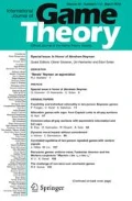
Bahel and Trudeau (2018) study a class of games (called Production Allocation Games) where agents, who demand different quantities of a given good, have individual technologies that they put in common to efficiently produce their demands. The authors examine technologies with increasing or decreasing returns to scale. Example 1 is a special case where the individual technologies are all linear.
Observe that, since the pattern \(h^{m}\) is symmetric, the shares remain the same no matter how we order/label these \(x(N)+|N_{0}(x)|\) units.
We thank the Associate Editor for suggesting this analysis.
Recall that the cost share of a technological agent for any pattern method is always individually rational, since the stand-alone cost is zero and the share is non-positive (by Strong Dummy) for such an agent.
We thank Hervé Moulin for drawing our attention to the class of homogeneous cost functions.
In words, Eq. (8) means that there exists a path (in the support of \(h^{m}\)) that compensates the technology of i at z, when the jth unit of demand has been produced (which is why \( z_{j}=2 \) and \(z_{i}=1\)).
It is easy to check that R is indeed an equivalence relation.
Formally, this means that there exists \(k_{1},\ldots ,k_{m}\in \{1,\ldots ,2m\}\) s.t. \(k_{1}<\cdots <k_{m}\) and, for any \(h\in \{1,\ldots ,m\}\), we have \( \left\{ \begin{array}{ll} p_{i_{h}}(k_{h})=1, &{} \\ p_{i_{h}}(k_{h}-1)=0. &{} \end{array} \right. \)
Recall that each unit \(k\in I_{i}\) possesses the full technology of agent i .
We remind the reader that (i) the first unit for any \(r\in [0,2e]\) represents the technology and (ii) a costless unit is added to the null demand of any technological agent \(i\in N_{0}(x)\).
References
Aumann RJ, Shapley L (1974) Values of nonatomic games. Princeton University Press, Princeton
Bahel E (2011) The implications of the ranking axiom for discrete cost sharing methods. Int J Game Theory 40:551–589
Bahel E, Trudeau C (2013) A discrete cost sharing model with technological cooperation. Int J Game Theory 42:439–460
Bahel E, Trudeau C (2014a) Stable lexicographic rules for shortest path games. Econ Lett 125:266–269
Bahel E, Trudeau C (2014b) Shapley-Shubik methods in cost sharing problems with technological cooperation. Soc Choice Welf 43:261–285
Bahel E, Trudeau C (2018) Stable cost sharing in production allocation games. Rev Econ Design 22:25–53
Bakirtzis A (2001) Aumann–Shapley transmission congestion pricing. IEEE Power Eng Rev 21:67–69
Bhattacharya S, d’Aspremont C, Guriev S, Sen D, Tauman Y (2014) Cooperation in R&D: patenting, licensing and contracting. In: Chatterjee K, Samuelson W (eds) Game theory and business applications. Springer, New York
Billera L, Heath D, Raanan J (1978) Internal telephone billing rates: A novel application of nonatomic game theory. Oper Res 26:956–965
Bird C (1976) On cost allocation for a spanning tree: a game theoretic approach. Networks 6:335–350
Calvo E, Santos JC (2000) A value for multichoice games. Math Soc Sci 40:341–354
Friedman E, Moulin H (1999) Three methods to share joint costs or surplus. J Econ Theory 87:275–312
Haimanko O, Tauman Y (2002) Recent developments in the theory of Aumann–Shapley pricing, part I: the nondifferentiable case. In: Thomson W (ed) Game theory and resource allocation: the axiomatic approach. NATO ASI Series
Junqueira M, da Costa LC, Barroso LA, Oliveira GC, Thome LM, Pereira MV (2007) An Aumann–Shapley approach to allocate transmission service cost among network users in electricity markets. IEEE T Power Syst 22:1532–1546
Kishimoto S, Watanabe N, Muto S (2011) Bargaining outcomes in patent licensing: asymptotic results in a general Cournot market. Math Soc Sci 61:114–123
Layne-Farrar A, Lerner J (2011) To join or not to join: examining patent pool participation and rent sharing rules. Int J Ind Organ 29:294–303
Lerner J, Tirole J (2004) Efficient patent pools. Am Econ Rev 94:691–711
Moulin H (1995) On additive methods to share joint costs. Jpn Econ Rev 46:303–332
Moulin H, Shenker S (1999) Distributive and additive costsharing of an homogeneous good. Games Econ Behav 27:299–330
Moulin H, Sprumont Y (2007) Fair allocation of production externalities: recent results. Rev Polit 117:7–37
Myerson R (1980) Conference structures and fair allocation rules. Int J Game Theory 9:169–182
van den Nouweland A, Potters J, Tijs S, Zarzuelo J (1995) Cores and related solution concepts for multi-choice games. Math Meth Oper Res 41:289–311
Petrosyan L, Zaccour G (2003) Time-consistent Shapley value allocation of pollution cost reduction. J Econ Dyn Control 27:381–398
Powers MR (2007) Using Aumann–Shapley values to allocate insurance risk. N Am Actuar J 11:113–127
Rosenthal EC (2013) Shortest path games. Eur J Oper Res 224:132–140
Samet D, Tauman Y, Zang I (1984) An application of the Aumann–Shapley prices for cost allocation in transportation problems. Math Oper Res 9:25–42
Sprumont Y (2005) On the discrete version of the Aumann–Shapley cost-sharing method. Econometrica 73:1693–1712
Sprumont Y (2008) Nearly serial sharing methods. Int J Game Theory 37:155–184
Tauman Y, Watanabe N (2007) The Shapley value of a patent licensing game: the asymptotic equivalence to non-cooperative results. Econ Theory 30:135–149
Wang Y (1999) The additivity and dummy axioms in the discrete cost sharing model. Econ Lett 64:187–192
Watanabe N, Muto S (2007) Stable profit sharing in a patent licensing game: general bargaining outcomes. Int J Game Theory 37:505–523
Acknowledgements
The authors thank Hervé Moulin and Yves Sprumont for stimulating conversations. The thoughtful comments and suggestions of two anonymous referees and an associate editor have helped improve the paper. Financial support from the Social Sciences and Humanities Research Council of Canada (SSHRC) is gratefully acknowledged [Grant Number 435-2014-0140].
Author information
Authors and Affiliations
Corresponding author
Ethics declarations
Conflicts of interest
Authors have carefully complied with the ethical standards of the journal and are free of conflicts of interests.
Appendix
Appendix
1.1 Figures

An example of a pattern method for \(m=3\)

Elementary flows \(f^{\mathcal {S}_{{\tiny pub} }^{m}}\) and \(f^{\mathcal {S}_{pr}^{m}}\) for \(m=3\)

Remaining elementary flows for \(m=3\)
1.2 Additional computations for Example 3
Let us calculate the shares for agents 2 and 3. As previously discussed, \(\partial _{2}C^{u*}(t)=0\) for all t such that \( t_{2}=1\) and \(\partial _{3}C^{u*}(t)=0\) for all t such that \(t_{3}=2.\) The following table describes the marginal cost of the demand of agent 2 depending on the technologies and demands already introduced, as well as the flow associated to each of these marginal costs by the elementary flows \(f^{ \mathcal {S}_{{\tiny pub}}^{4}}\) and \(f^{\mathcal {S}_{{\tiny pr}}^{4}}\), associated respectively to the private and public Aumann–Shapley methods, as well as the elementary flow \(f^{\mathcal {S}_{{\tiny *}}^{4}}.\)
r | \(\partial _{2}C^{u*}(r)\) | \(f_{2}^{\mathcal {S}_{{\tiny pub}}^{4}}(r)\) | \(f_{2}^{\mathcal {S}_{{\tiny pr}}^{4}}(r)\) | \(f_{2}^{\mathcal {S}_{{\tiny *}}^{4}}(r)\) |
(0, 0, 2, 0) | 2 | 0 | \(\frac{1}{4}\) | 0 |
(1, 0, 2, 0) | 2 | 0 | 0 | \(\frac{1}{12}\) |
(0, 1, 2, 0) | 2 | 0 | 0 | \(\frac{1}{12}\) |
(0, 0, 2, 1) | 1 | 0 | 0 | \(\frac{1}{12}\) |
(1, 1, 2, 0) | 2 | 0 | 0 | 0 |
(1, 0, 2, 1) | 1 | 0 | 0 | 0 |
(0, 1, 2, 1) | 1 | 0 | 0 | 0 |
(1, 1, 2, 1) | 1 | \(\frac{1}{4}\) | 0 | 0 |
(2, 0, 2, 0) | 2 | 0 | \(\frac{1}{12}\) | 0 |
(0, 2, 2, 0) | 2 | 0 | \(\frac{1}{12}\) | 0 |
(0, 0, 2, 2) | 1 | 0 | \(\frac{1}{12}\) | 0 |
(2, 1, 2, 0) | 2 | 0 | 0 | \(\frac{1}{24}\) |
(2, 0, 2, 1) | 1 | 0 | 0 | \(\frac{1}{24}\) |
(1, 2, 2, 0) | 2 | 0 | 0 | \(\frac{1}{24}\) |
(0, 2, 2, 1) | 1 | 0 | 0 | \(\frac{1}{24}\) |
(1, 0, 2, 2) | 1 | 0 | 0 | \(\frac{1}{24}\) |
(0, 1, 2, 2) | 1 | 0 | 0 | \(\frac{1}{24}\) |
(2, 2, 2, 0) | 2 | 0 | \(\frac{1}{12}\) | 0 |
(2, 0, 2, 2) | 1 | 0 | \(\frac{1}{12}\) | 0 |
(0, 2, 2, 2) | 1 | 0 | \(\frac{1}{12}\) | 0 |
(2, 1, 2, 1) | 1 | \(\frac{1}{12}\) | 0 | 0 |
(1, 2, 2, 1) | 1 | \(\frac{1}{12}\) | 0 | 0 |
(1, 1, 2, 2) | 1 | \(\frac{1}{12}\) | 0 | 0 |
(2, 2, 2, 1) | 1 | \(\frac{1}{12}\) | 0 | \(\frac{1}{12}\) |
(2, 1, 2, 2) | 1 | \(\frac{1}{12}\) | 0 | \(\frac{1}{12}\) |
(1, 2, 2, 2) | 1 | \(\frac{1}{12}\) | 0 | \(\frac{1}{12}\) |
(2, 2, 2, 2) | 1 | \(\frac{1}{4}\) | \(\frac{1}{4}\) | \(\frac{1}{4}\) |
We hence have \(AS_{2}^{{\tiny pub}}(P)=AS_{2}^{{\tiny pub} }(P^{u})=\sum \nolimits _{r\in [e^{2},2e]}f_{2}^{\mathcal {S}_{{\tiny pub} }^{4}}(r)\partial _{2}C^{u*}(r)=1\), and \(AS_{2}^{{\tiny pr}}(P)=AS_{2}^{ {\tiny pr}}(P^{u})=\sum \nolimits _{r\in [e^{2},2e]}f_{2}^{\mathcal {S}_{ {\tiny pr}}^{4}}(r)\partial _{2}C^{u*}(r)=\frac{3}{2}\). We also find \( y_{2}^{*}(P)=y_{2}^{*}(P^{u})=\sum \nolimits _{r\in [e^{2},2e]}f_{2}^{\mathcal {S}_{{\tiny *}}^{4}}(r)\partial _{2}C^{u*}(r)=\frac{5}{4}.\)
The following table describes the marginal cost of adding the technology of agent 3 depending on the technologies and demands already introduced, as well as the flow associated to each of these marginal costs by the elementary flows \(f^{\mathcal {S}_{{pub}}^{4}}\) and \(f^{\mathcal {S}_{{\small pr}}^{4}}\), associated respectively to the private and public Aumann–Shapley methods, as well as the elementary flow \(f^{\mathcal {S}_{{\small *} }^{4}}.\)
r | \(\partial _{3}C^{u*}(r)\) | \(f_{3}^{\mathcal {S}_{{\tiny pub}}^{4}}(r)\) | \(f_{3}^{\mathcal {S}_{{\tiny pr}}^{4}}(r)\) | \(f_{3}^{\mathcal {S}_{{\tiny *}}^{4}}(r)\) |
(0, 0, 0, 1) | 0 | \(\frac{1}{4}\) | 0 | \(\frac{1}{4}\) |
(1, 0, 0, 1) | 0 | \(\frac{1}{12}\) | 0 | \(\frac{1}{12}\) |
(0, 1, 0, 1) | 0 | \(\frac{1}{12}\) | 0 | \(\frac{1}{12}\) |
(0, 0, 1, 1) | 0 | \(\frac{1}{12}\) | 0 | \(\frac{1}{12}\) |
(1, 1, 0, 1) | 0 | \(\frac{1}{12}\) | 0 | 0 |
(1, 0, 1, 1) | 0 | \(\frac{1}{12}\) | 0 | 0 |
(0, 1, 1, 1) | 0 | \(\frac{1}{12}\) | 0 | 0 |
(1, 1, 1, 1) | 0 | \(\frac{1}{4}\) | 0 | 0 |
(2, 0, 0, 1) | − 1 | 0 | \(\frac{1}{12}\) | 0 |
(0, 2, 0, 1) | − 1 | 0 | \(\frac{1}{12}\) | 0 |
(0, 0, 2, 1) | − 1 | 0 | \(\frac{1}{12}\) | 0 |
(2, 1, 0, 1) | − 1 | 0 | 0 | \(\frac{1}{24}\) |
(2, 0, 1, 1) | − 1 | 0 | 0 | \(\frac{1}{24}\) |
(1, 2, 0, 1) | − 1 | 0 | 0 | \(\frac{1}{24}\) |
(0, 2, 1, 1) | − 1 | 0 | 0 | \(\frac{1}{24}\) |
(1, 0, 2, 1) | − 1 | 0 | 0 | \(\frac{1}{24}\) |
(0, 1, 2, 1) | − 1 | 0 | 0 | \(\frac{1}{24}\) |
(2, 2, 0, 1) | − 4 | 0 | \(\frac{1}{12}\) | 0 |
(2, 0, 2, 1) | − 2 | 0 | \(\frac{1}{12}\) | 0 |
(0, 2, 2, 1) | − 2 | 0 | \(\frac{1}{12}\) | 0 |
(2, 1, 1, 1) | − 1 | 0 | 0 | 0 |
(1, 2, 1, 1) | − 1 | 0 | 0 | 0 |
(1, 1, 2, 1) | − 1 | 0 | 0 | 0 |
(2, 2, 1, 1) | − 4 | 0 | 0 | \(\frac{1}{12}\) |
(2, 1, 2, 1) | − 2 | 0 | 0 | \(\frac{1}{12}\) |
(1, 2, 2, 1) | − 2 | 0 | 0 | \(\frac{1}{12}\) |
(2, 2, 2, 1) | − 5 | 0 | \(\frac{1}{4}\) | 0 |
Taking the scalar product of column with the following ones, we obtain agent 3’s respective shares: \(AS_{3}^{{\tiny pub}}(P)=AS_{3}^{{\tiny pub}}(P^{u})=\sum \nolimits _{r\in [e^{3},2e]}f_{3}^{\mathcal {S}_{{\tiny pub}}^{4}}(r)\partial _{3}C^{u*}(r)=0\), \(AS_{3}^{{\tiny pr}}(P)=AS_{3}^{ {\tiny pr}}(P^{u})=\sum \nolimits _{r\in [e^{3},2e]}f_{3}^{\mathcal {S}_{ {\tiny pr}}^{4}}(r)\partial _{3}C^{u*}(r)=-\frac{13}{6}\) and \( y_{3}^{*}(P)=y_{3}^{*}(P^{u})=\sum \nolimits _{r\in [e^{3},2e]}f_{3}^{\mathcal {S}_{*}^{4}}(r)\partial _{3}C^{u*}(r)=- \frac{11}{12}.\)
1.3 Proofs of the Theorems
1.3.1 Theorem 2
Suppose y is a pattern method represented by a sequence of patterns \(h=\left( h^{m}\right) _{m\ge 2}.\)
Step 1 Showing that pattern methods satisfy NMS and ID
Substep 1a Pattern methods satisfy NMS
Consider \(P=(N,x,C)\), \(P^{\prime }=(N^{\prime },C^{\prime },x^{\prime })\in P\) such that \(P^{\prime }\) is a splitting manipulation of P available to some agent \(i\in N\), with \(N^{\prime }=(N{\setminus } i)\cup I\) . First, observe that \(m=\sum _{j\in N\backslash i}x_{j}+x_{i}+\left| N_{0}(x)\right| =\sum _{j\in N\backslash i}x_{j}^{\prime }+\sum _{j\in I}x_{j}^{\prime }+\left| N_{0}(x^{\prime })\right| =m^{\prime }\) by the properties of a splitting manipulation. We thus have that,
as \(m=m^{\prime }\) and the fact that \(P^{\prime }\) is a splitting manipulation of P.
We also need to show that it does not affect the shares of agents in \(N\backslash i.\) Consider agent \(j\in N\backslash i.\) Clearly, since \(m=m^{\prime }\) and \(x_{j}=x_{j}^{\prime },\) we have that \( y_{j}^{h_{m}}(N,x,C)=y_{j}^{h_{m}}(N^{\prime },C^{\prime },x^{\prime }).\)
Substep 1b Pattern methods satisfy ID
Suppose that i is a demand dummy in problem \(P=(N,x,C),\) with \(x_{i}=1.\) Consider the problem \(P^{\prime }=(N,C^{\prime },\left( 0_{i},x_{N\backslash i}\right) )\) where \(C^{\prime }\) is the restriction of C to \(\left[ 0,e^{N}+x_{N\backslash i}\right] .\) Since agent i is a demand dummy, we have that \((N^{u},x^{u},C^{u})=(N^{u}, \left( 0_{i},x_{N\backslash i}\right) ^{u},\left( C^{\prime }\right) ^{u})\) and thus that \(y_{i}^{h_{m}}(N,x,C)= \sum _{k=1}^{x_{i}}y_{i_{k}}^{h_{m}}(N^{u},x^{u},C^{u})=y_{i_{1}}^{h_{m}}(N^{u}, x^{u},C^{u}) \) while \(y_{i}^{h_{m}}(N, \left( 0_{i},x_{N\backslash i}\right) , C)=y_{i_{1}}^{h_{m^{\prime }}}(N^{u},x^{u},C^{u}).\) Since \(m=m^{\prime },\) we have that \(y_{i}^{h_{m}}(N,x,C)=y_{i}^{h_{m}}(N,\left( 0_{i},x_{N\backslash i}\right) ,C )\) and \( y_{j}^{h_{m}}(N,x,C)=y_{j}^{h_{m}}(N,\left( 0_{i},x_{N\backslash i}\right) ,C )\) for all \(m\in N\backslash i.\)
Step 2 Showing that a flow method that satisfies NMS and ID is a pattern method.
Consider a problem (N, x, C) where, without loss of generality, the first K agents in N have \(x_{i}>0\) while the remaining ones have null demands.
Substep 2a
Since y meets no merging or splitting, we can write
where \(P^{(1)}\) is the problem obtained from P by splitting the demand of agent 1 into \(x_{1}\) distinct (unitary) demands of 1. We have: \( P^{(1)}=(N^{(1)},x^{(1)},C^{(1)})\), where
By the same token, starting from the problem \(P^{(1)}\) and splitting the demand of agent 2 into \(x_{2}\) unitary demands gives:
Combining, we obtain
Using the same argument repeatedly (K times, in fact), we get:
Substep 2b
Since y meets irrelevant demand, we can write
where \(\bar{P}^{(K+1)}\) is the problem obtained from \(P^{(K)}\) by adding a costless unit of demand to agent \(K+1\). We have: \(\bar{P}^{(K+1)}=(N^{(K)}, \bar{x}^{(K+1)},\bar{C}^{(K+1)})\), where \(\bar{x}^{(K+1)}=\left( 1,x_{N^{(K)}{\setminus } K+1}^{(K)}\right) \) and \(\bar{C}^{(K+1)}\) is such that for all \(t\in \left[ 0,z^{N^{(K)}{\setminus } K+1}\right] ,\)
Combining with the previous substep, we obtain
Repeating the argument \(n-\left| K\right| \) times, we obtain
where \(\bar{P}^{(n)}=(N^{(K)},\bar{x}^{(n)},\bar{C}^{(n)})\) and
Thus, \(\bar{P}^{(n)}=(N^{u},x^{u},C^{u})\) and \(\left\{ \begin{array}{ll} y_{i}(N,x,C)=\sum \limits _{k=1}^{x_{i}}y_{i_{k}}(N^{u},x^{u},C^{u}), &{}\quad \mathrm{if }\;x_{i}>0; \\ y_{i}(N,x,C)=y_{i}(N^{u},x^{u},C^{u}), &{}\quad \mathrm{if }\;x_{i}=0. \end{array} \right. ~~\) \(\square \)
1.3.2 Theorem 3
(i) \(AS^{pub}\) satisfies Fair Rent
Consider a problem (N, x, C) s.t. \(N_{0}(x)\equiv N{\setminus } N(x)\ne \emptyset \). By definition of \(\mathcal {S}_{pub}^{m}\) we have \(p(m)=e\), for \( m=|N_{0}(x)|+x(N)\) and \(p\in \mathcal {S}_{pub}^{m}\); and therefore each technological agent \(i\in N_{0}(x)\) receives a null rent under the public Aumann–Shapley rule: \(y_{i}(N,x,C)=0,\forall i\in N_{0}(x)\). Thus, we have by efficiency,
and hence Fair Rent is satisfied by \(AS^{pub}\). Note that the inequality above comes from Property 1 of our cost functions with technological cooperation (see Sect. 2).
(ii) All other pattern methods violate Fair Rent
Suppose now that we have a pattern method \(y\ne AS^{pub}\) that is represented by the symmetric flow \(h^{m}\) (for each \(m\in \mathrm {IN}\)) on the box [0, 2e]. First, note from Definitions 5 and 6 that \(y\ne AS^{pub}\) implies that there exists \(m\ge 2\) and \(z\in [0,2e]\) such that:Footnote 7
Next, pick any problem (N, x, C) s.t. \(|N_{0}(x)|+x(N)=m\), \(i\in N_{0}(x)\) [\( x_i=0\)], \(x_j=1\), and \(\partial C^{u*}(z)<\frac{C^{*}(z^{x})-C^{*}((z^{x})^{N(x)})}{h_{i}^{m}(2e,z)}\). Then, since \(i\in N_{0}(x)\) and \( \partial _{i}C^{u*}(r)\le 0\) (from \(x_{i}=0\)), we have
That is to say,
Therefore, Fair Rent is not met by y. \(\square \)
1.3.3 Theorem 4
-
(i)
\(AS^{pub}\) does not meet LBR. Fix \(N\in \mathcal {N}\) and \(x\in \mathrm {IN}^{N}\); and suppose that \(i\in N_{0}(x)\), with \(\left| C(N,x)-C\left( N{\setminus } i,x_{N{\setminus } i}\right) \right| >0\). Since \(AS_{i}^{pub}(N,x,C)=0\), we can claim that
$$\begin{aligned} \left| AS_{i}^{pub}(N,x,C)\right| =0<k\left| C(N,x)-C\left( N{\setminus } i,x_{N{\setminus } i}\right) \right| ,\quad \forall k\in (0,1). \end{aligned}$$Hence, \(AS^{pub}\) violates LBR.
-
(ii)
\(AS^{pr}\) satisfies \(\frac{1}{m}\)-LBR. Fix \(N\in \mathcal {N}\), \(x\in \mathrm {IN}^{N}\) and let \(m\equiv |N_{0}(x)|+x(N)\). Next consider \(i\in N_{0}(x)\) and, for any path \( p:\{0,1,\ldots ,z_{1}^{x}+\cdots +z_{m}^{x}\}\rightarrow [0,2e]\), denote by \(k_{i}^{p}\in \{0,1,\ldots ,z_{1}^{x}+\cdots +z_{m}^{x}\}\) the unique number such that \(p_{i}(k_{i}^{p})=1\) and \(p_{i}(k_{i}^{p}-1)=0\). Using this notation and the definition of \(AS^{pr}\), we may then write:
Note that \(p(k_{i}^{p})=2e-e^{i}\) means that the technology of i is activated last, when the demands of all other agents have already been produced. That is to say, \(\partial _{i}C^{u*}(p(2e-e_{i}))=C(N,x)-C\left( N{\setminus } i,x_{N{\setminus } i}\right) \le 0\). Substituting in (9), we get:
A basic combinatorics exercise allows to see that we have exactly \((m-1)!\) paths \(p:\{0,1,\ldots ,z_{1}^{x}+\cdots +z_{m}^{x}\}\rightarrow [0,2e] \) such that \(p(k_{i}^{p})=2e-e^{i}\). Therefore, (11) becomes:
Since both the right and left hand sides are nonpositive, taking the absolute value gives \(|AS_{i}^{pr}(N,x,C)|\ge \frac{1}{m}\left| C(N,x)-C\left( N{\setminus } i,x_{N{\setminus } i}\right) \right| \), which is the desired result. \(\square \)
1.3.4 Theorem 6
Fix a separable problem \(P=(N,x,C)\), with \(C(S,t_{S})=M(|S|) \tilde{C} (t(S))\) and \(N_{0}(x)\ne \emptyset \), and recall that \( m\equiv |N^{u}|\). Using Theorem 2, it is sufficient to show that \(| y^{f}_{i}(P)| \le | AS^{pr}_{i}(P)| \), for any symmetric flow f to \(2e^{m}\) and any \(i\in N_{0}(x)\). We proceed in 4 steps.
1. It is well known that every flow f (to some \(z\in \mathbb {R}^{m}\)) can be written as a convex combination of paths (to z). In other words, denoting by \(\mathcal {P}^{z}\) the set of paths to z, one can write
Moreover, it is not difficult to see that, for every symmetric flow f, any two symmetric paths p and \(p^{\prime }\) (i.e., p and \( p^{\prime }\) are permutations of one another) will be given the same weight under the decomposition (12). More precisely, if we call \( \mathcal {S}(p)\) the class of paths that can be obtained as a permutation of p, we have \(\beta ^{p^{\prime }}=\beta ^{p}\), for any \(p^{\prime }\in \mathcal {S}(p)\). Let then \(\mathcal {S}_{1},\ldots ,\mathcal {S}_{L}\) be the list of equivalence classes for the equivalence relation R defined on \( \mathcal {P}^{z}\) by:Footnote 8 \( pRp^{\prime }\Leftrightarrow p^{\prime }\in \mathcal {S}(p)\). Recall that we have already introduced \(\mathcal {S}_{1}\) and \(\mathcal {S}_{2}\) in Sect. 4, when defining the public and private Aumann–Shapley methods. Using this partition of \(\mathcal {P}^{z}\) into equivalence classes and defining \(\beta (\mathcal {S}_{l})\equiv \beta ^{p}\) (for any \(p\in \mathcal {S}_{l}\)), one can then rewrite (12) as
In addition, since there are exactly m! possible permutations for any path to \(z\in \mathbb {R}^{m}\), we deduce from (13) that
Hence, defining \(\tilde{\beta }(\mathcal {S}_{l})=m!\beta (\mathcal {S}_{l})\), we may rewrite (14) as
For any \(l=1,\ldots ,L\), observe that \(f^{\mathcal {S}_{l}}\equiv \sum \nolimits _{p\in \mathcal {S}_{l}}\frac{p}{m!}\) is a symmetric flow to z since it is the average of all paths (to z) contained in \(\mathcal {S}_{l}\) . We call this symmetric flow the elementary flow (to z) associated with \(\mathcal {S}_{l}\). In other words, Eqs. (16) and (15) mean that any symmetric flow (to z) can be decomposed as a convex combination of elementary flows (to z).Footnote 9 Thus, to prove Theorem 6, it suffices to show that, the private Aumann–Shapley flow (\(f^{\mathcal {S}^{2}}\)) minimizes the technological players’ shares within the class of elementary flows to \(z=2e^{m}\).
2. Fix \(l=1,\ldots ,L\). We will now construct a one-to-one mapping \(\hat{\cdot }:\mathcal {S}_{l}\rightarrow \mathcal {S}_{2}\) . Let then \(p\in \mathcal {S}_{l}\) and consider the ordering \( \sigma ^{p}=[i_{1},i_{2},\ldots ,i_{m}]\) according to which the technologies of the m unit-players are activated under the path p.Footnote 10 Observe that the path
is the unique path in \(\mathcal {S}_{2}\) that activates technological units in the same order as p. In addition, for any distinct \( p,p^{\prime }\in \mathcal {S}_{l}\), we have \(\hat{p}\ne \hat{p}^{\prime }\). Therefore, \(\hat{\cdot }\) is a one-to-one mapping (since \(\mathcal {S}_{l}\) and \(\mathcal {S}_{2}\) each have exactly m! elements).
3. For any path p (to 2e) and any \(r\in [0,2e]\subset \mathbb {R}^{m}\), define
The set t(r) describes the (actual) technologies that are available when the path p reaches r,Footnote 11 whereas q(r) gives the number of costly units that have been produced when p reaches the profile r.Footnote 12 In addition, letting \( k_{i}^{p}\) be the (unique) index \(k\in \{1,\ldots ,2m\}\) s.t. \(p_{i}(k)=1\) and \(p_{i}(k-1)=0\), one can see from (17) to (19) that,
4. We now show that, for any \(i\in N_{0}(x)\), \(l=1,\ldots ,L \) and \(p\in \mathcal {S}_{l}\), we have \(y^{p}_{i}(P)\ge y^{\hat{ p}}_{i}(P)\). That is to say, a technological agent i always receives under p a higher share than under \(\hat{p}\).
Let us then fix \(i\in N_{0}(x)\), \(l=1,\ldots ,L\) and \(p\in \mathcal {S}_{l}\). Using the notation above, Eq. (20) and the fact that P is a separable problem, one can compute the shares associated with the paths p and \(\hat{p}\) (for any \(i\in N_{0}(x)\ne \emptyset \)):
Hence, \(y^{p}_{i}(P)\ge y^{\hat{p}}_{i}(P)\), for any \(p\in \mathcal {S}_{l}\); and we can then write:
This proves that the private Aumann–Shapley method always minimizes (maximizes) the share (rent) of the technological agents among symmetric flow methods.
To conclude the proof, note that the inequality in (21) is strict whenever \(\tilde{C}\) is increasing and \( q(p(k_{i}^{p}))<q(\hat{p}(k_{i}^{\hat{p}})))\), which will happen—for at least one homogeneous problem (N, x, C), one equivalence class \(\mathcal {S} _{l}\), and one path \(p\in \mathcal {S}_{l}\)—as soon as the considered method y differs from \(AS^{pr}\). \(\square \)
Rights and permissions
About this article

Cite this article
Bahel, E., Trudeau, C. Consistency requirements and pattern methods in cost sharing problems with technological cooperation. Int J Game Theory 47, 737–765 (2018). https://doi.org/10.1007/s00182-018-0636-8
Accepted:
Published:
Issue Date:
DOI: https://doi.org/10.1007/s00182-018-0636-8