A New Fault Diagnosis Method for a Diesel Engine Based on an Optimized Vibration Mel Frequency under Multiple Operation Conditions

Abstract
:
1. Introduction
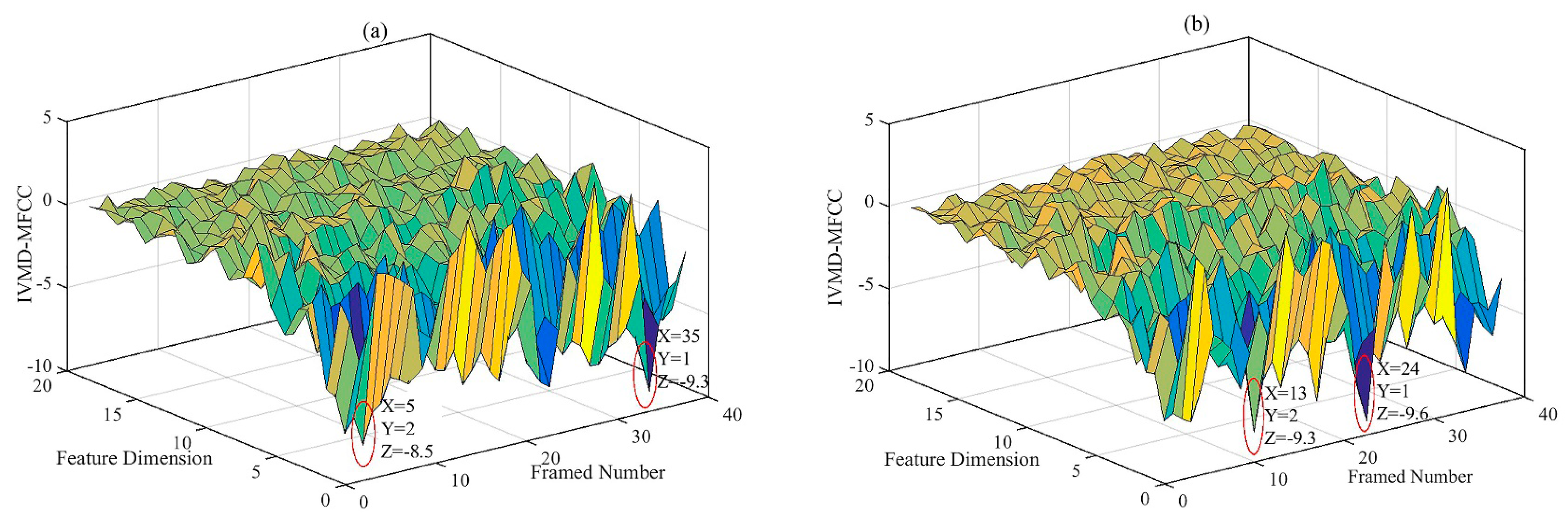
- In order to overcome the interference of complex operation conditions, this paper presents a novel representative feature from vibration signals by incorporating VMD into the effective adaptive decomposition of non-stationary signals to combine it with the excellent feature representation of MFCC.
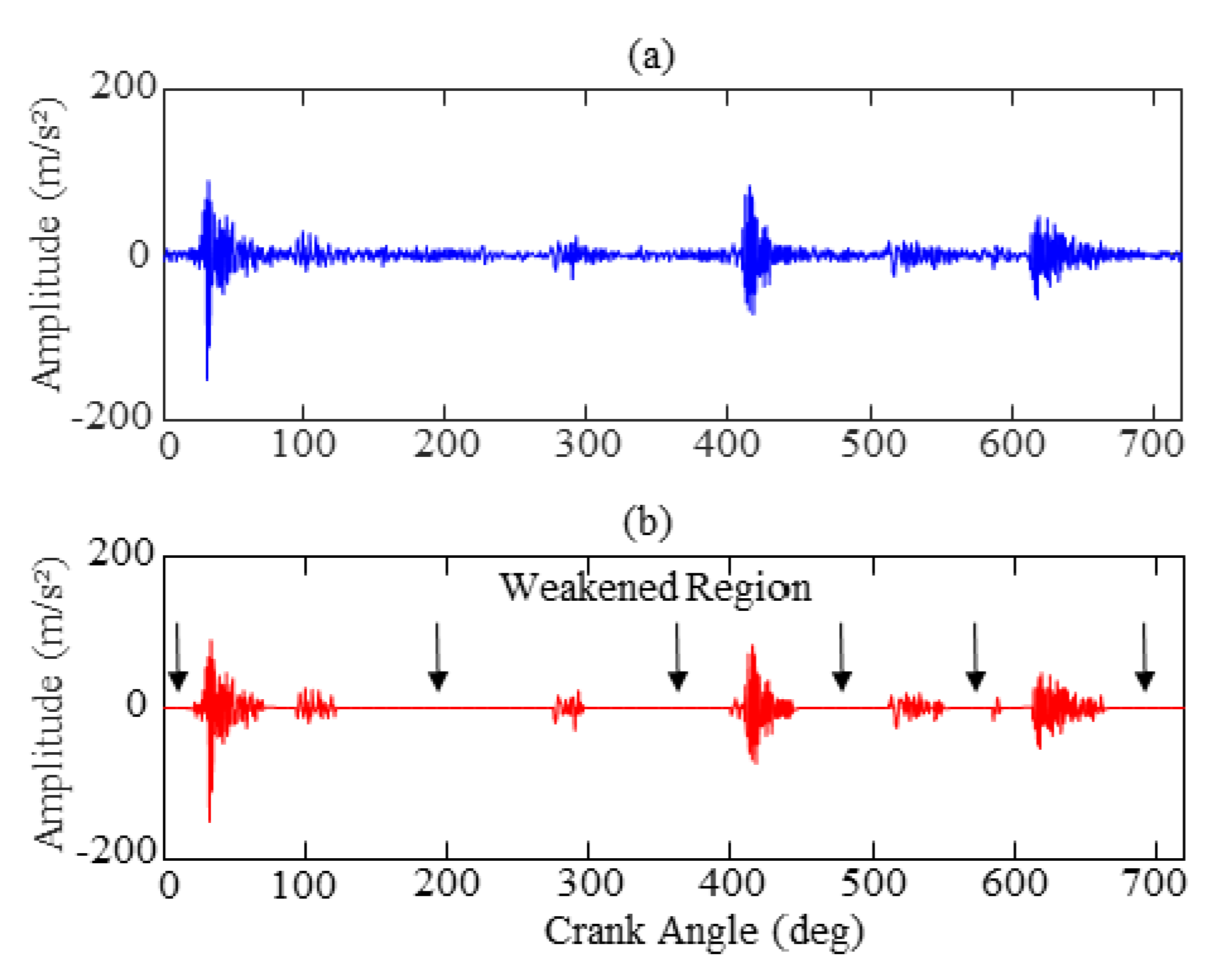
- In order to wipe out the strong noise and enhance signal improvement, an adaptive correlation threshold method is first proposed to weaken the invalid data before the feature extraction.
2. Diesel Engine Test-Bed and Signal Analysis
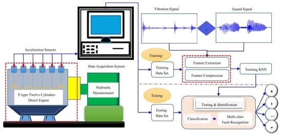
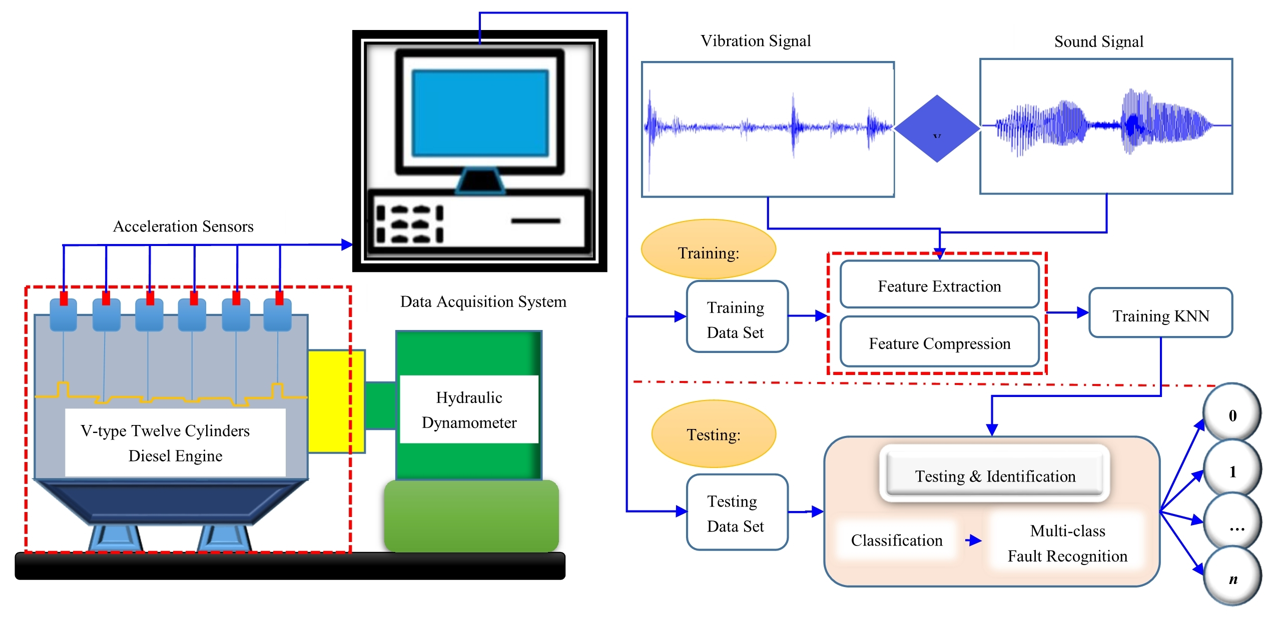
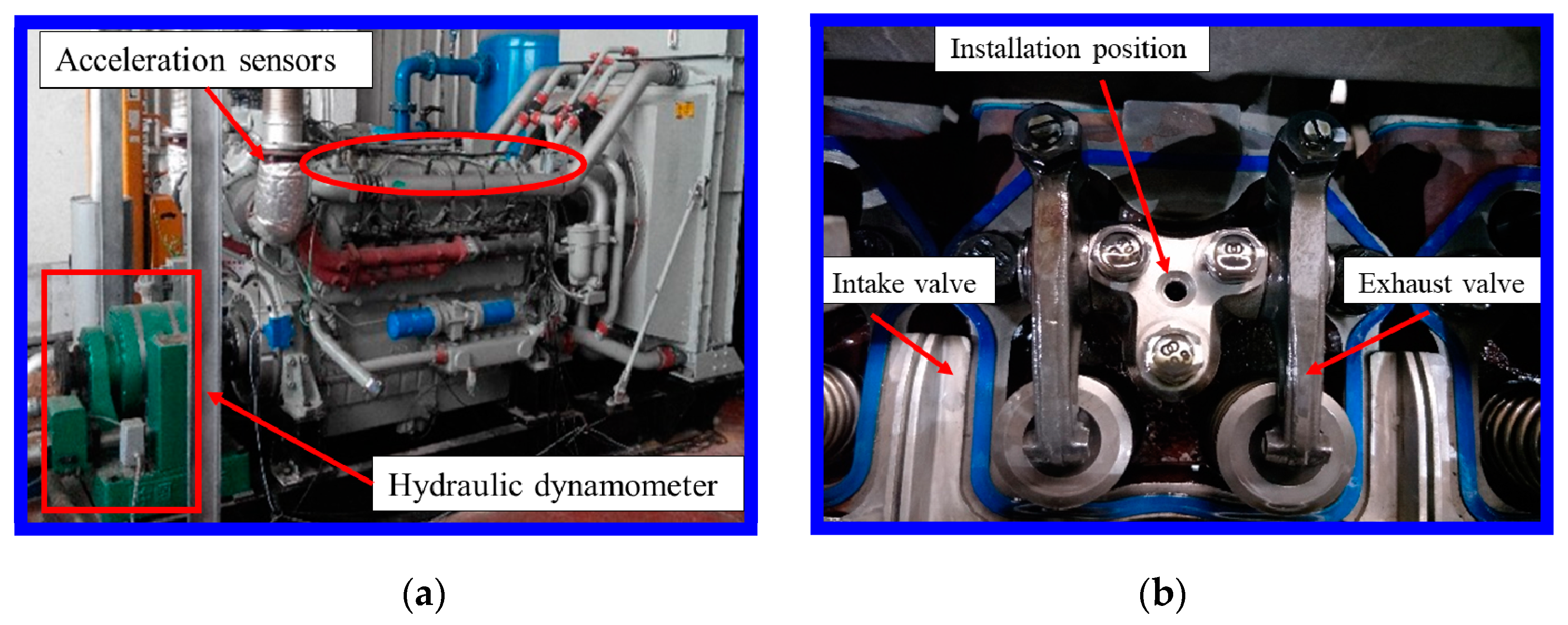
2.1. Diesel Engine Equipment and Data Acquisition
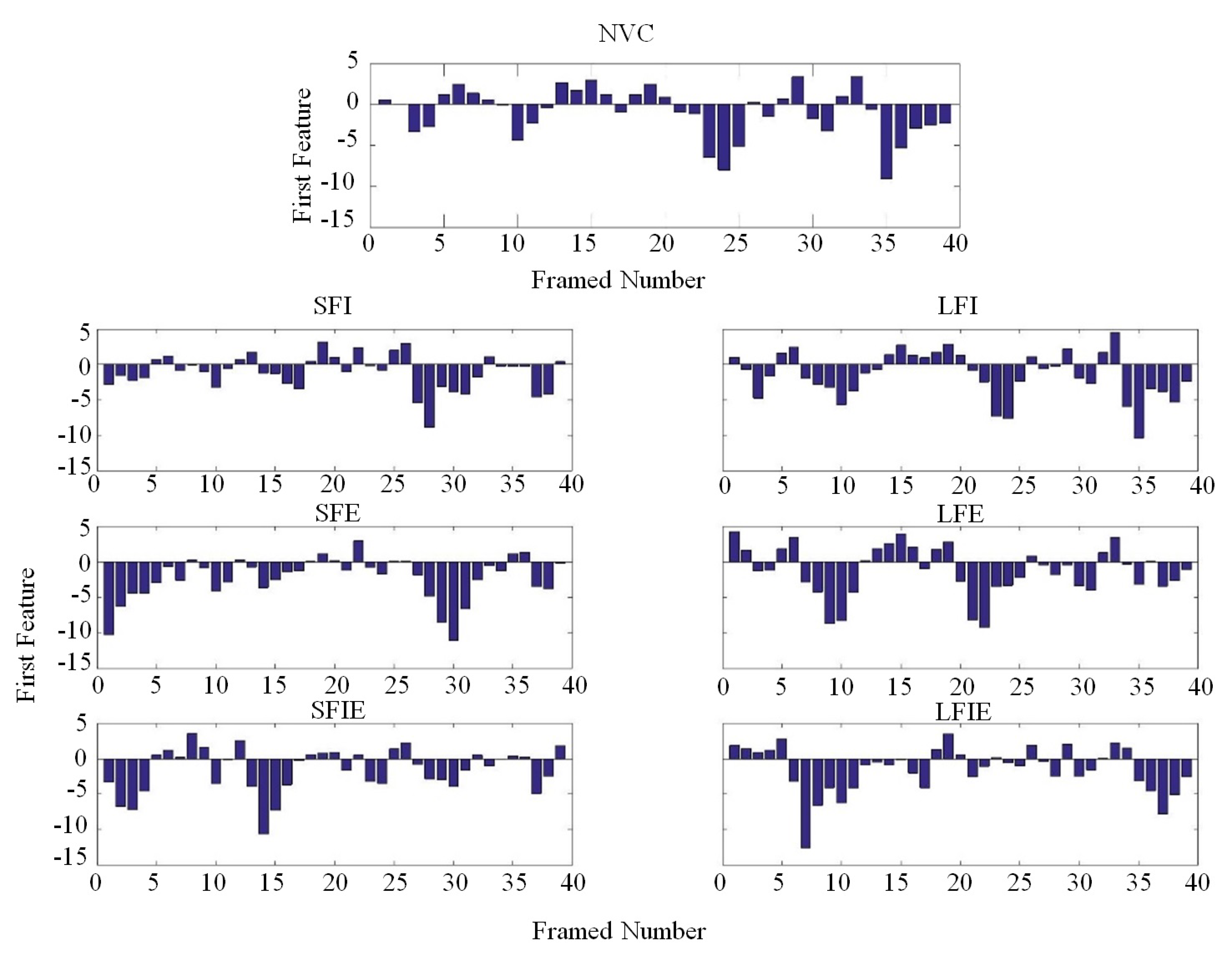
2.2. Establishment of Diesel Engine Valve Fault
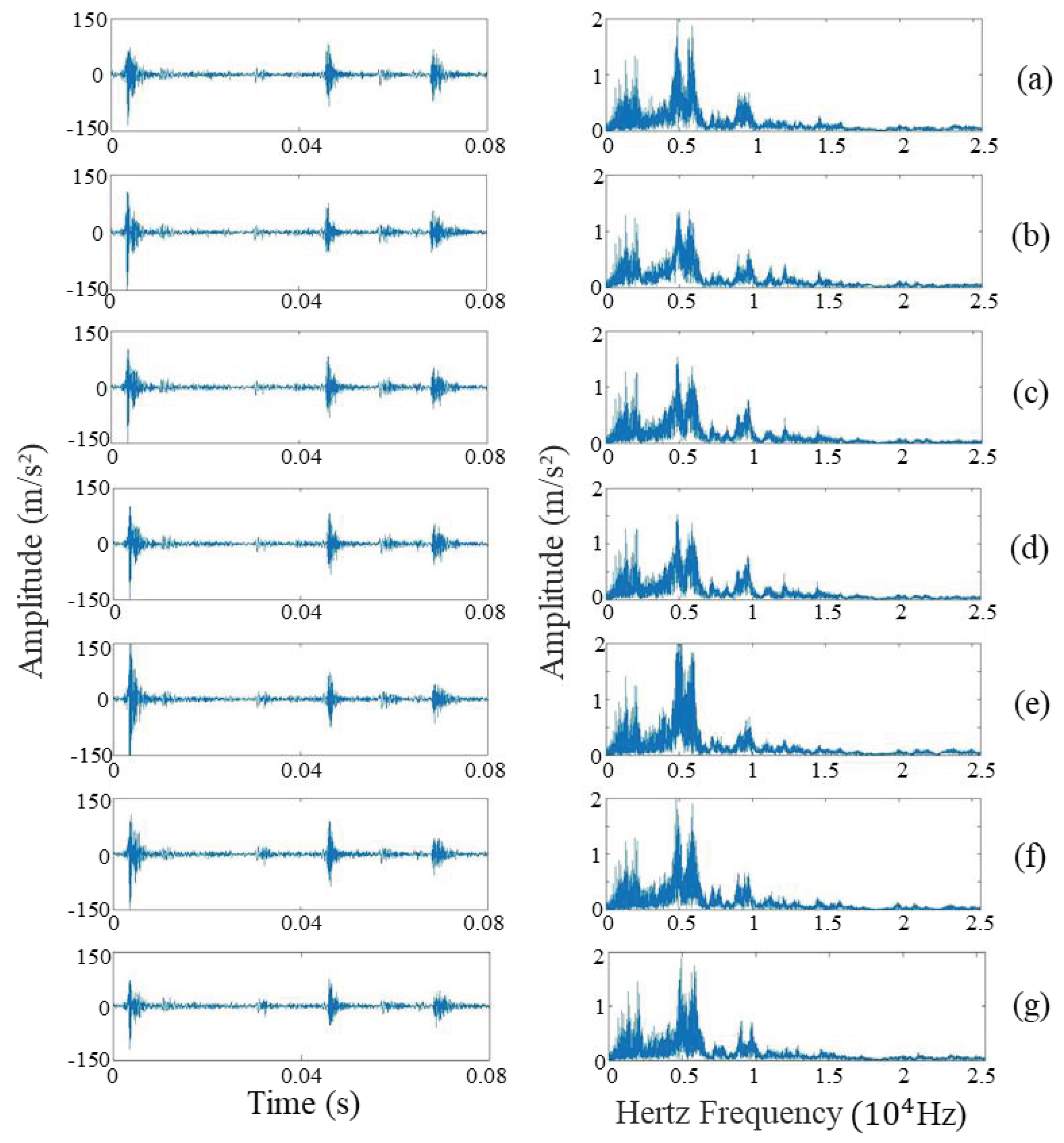
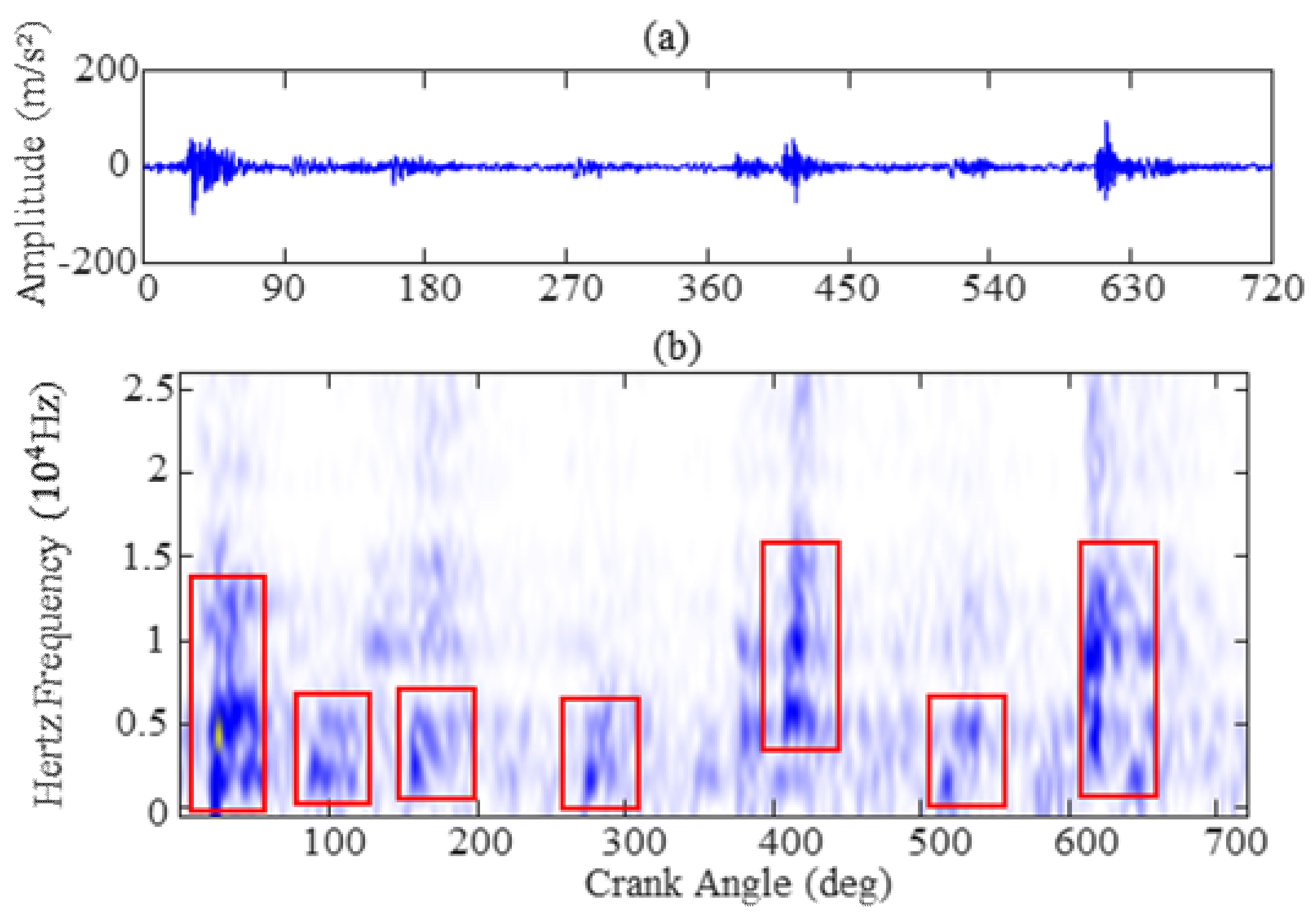
2.3. Time-Frequency of Sound and Vibration Signals
3. Methodology Based on Improved MFCC
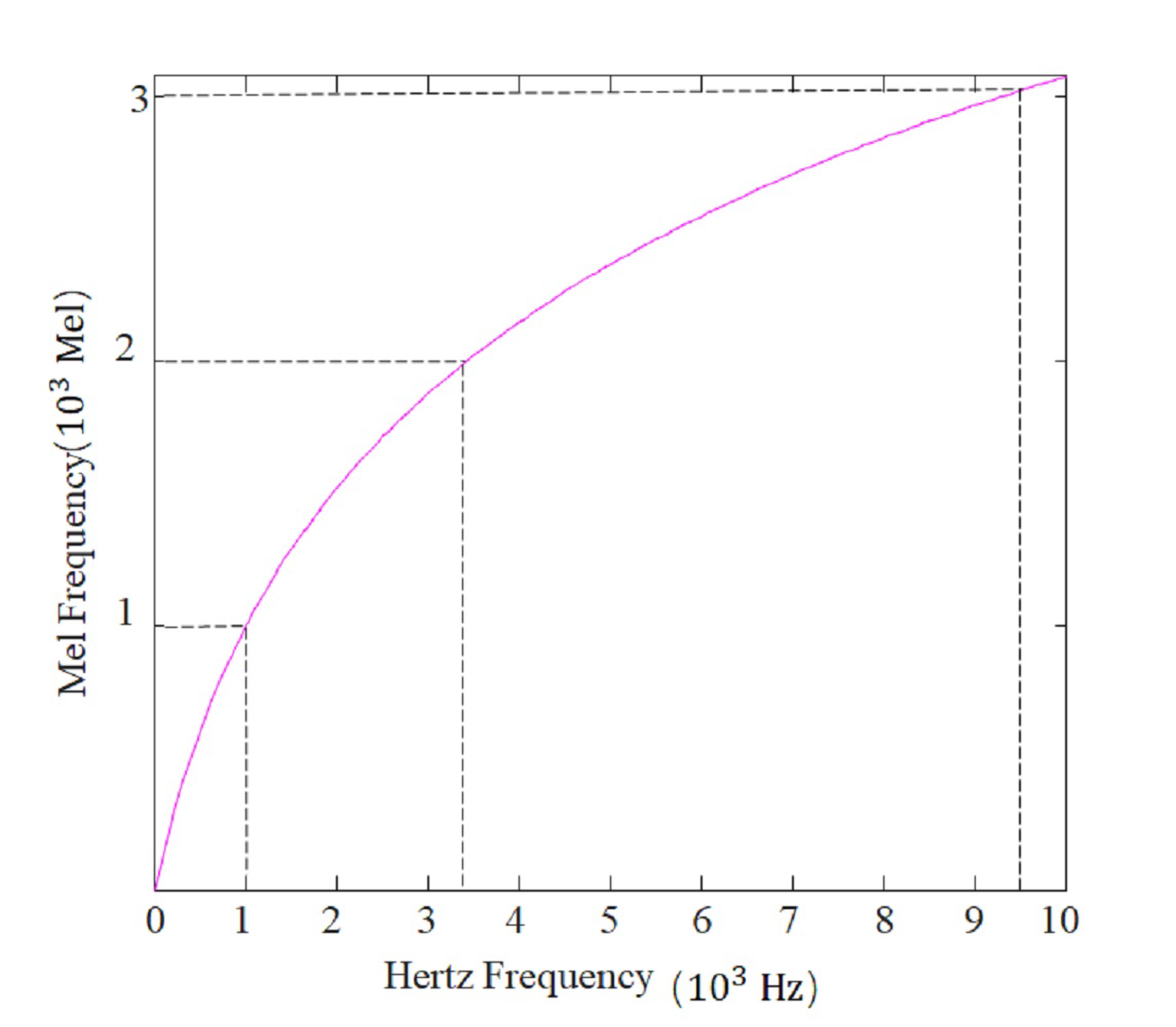
3.1. Mel Frequency Cepstrum Coefficient
3.2. Variational Mode Decomposition
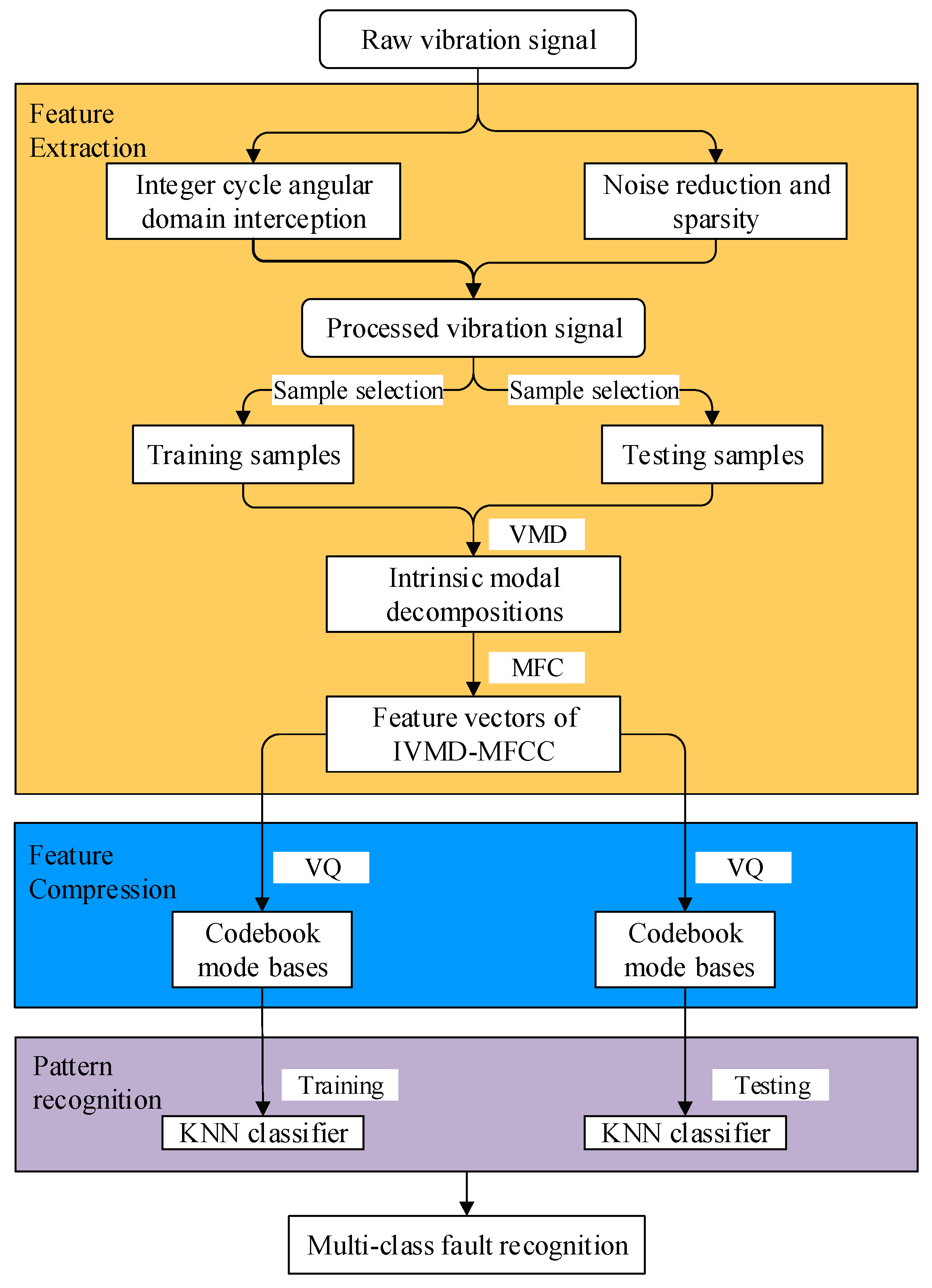
4. Comprehensive Procedure of the Proposed Method
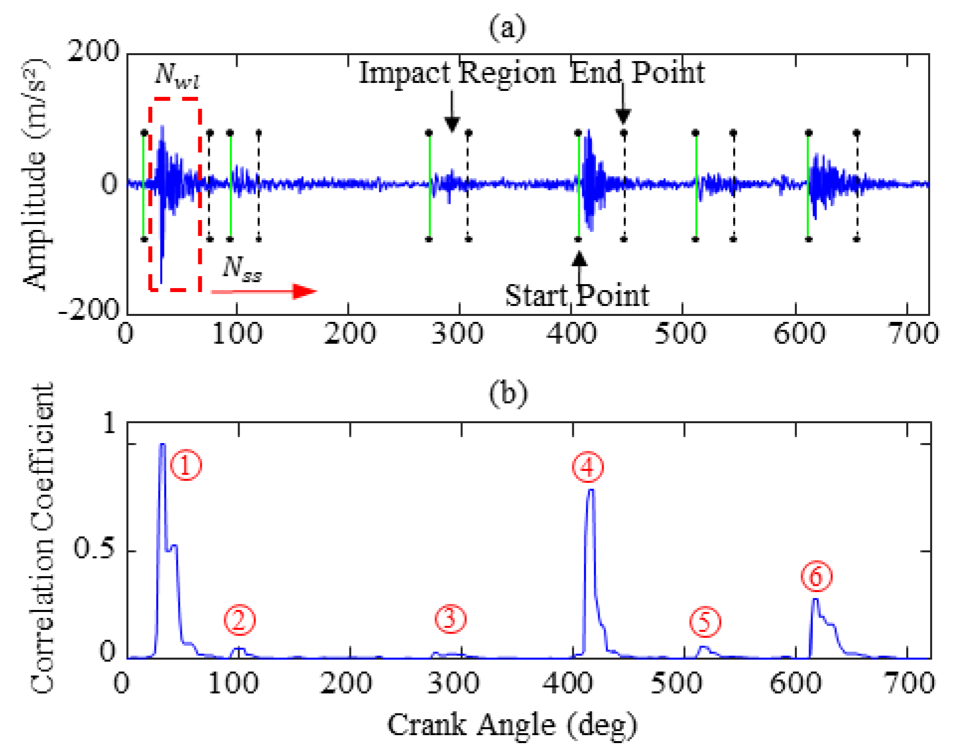
4.1. Signal Improvement
4.2. IVMD-MFCC
- Step 1: Input the raw signal x(t) and obtain a processed signal y(t) by utilizing the adaptive correlation threshold.
- Step 2: Initialize the parameters , , , n and step-wise decomposition by using VMD to obtain mode components (default k = 3).
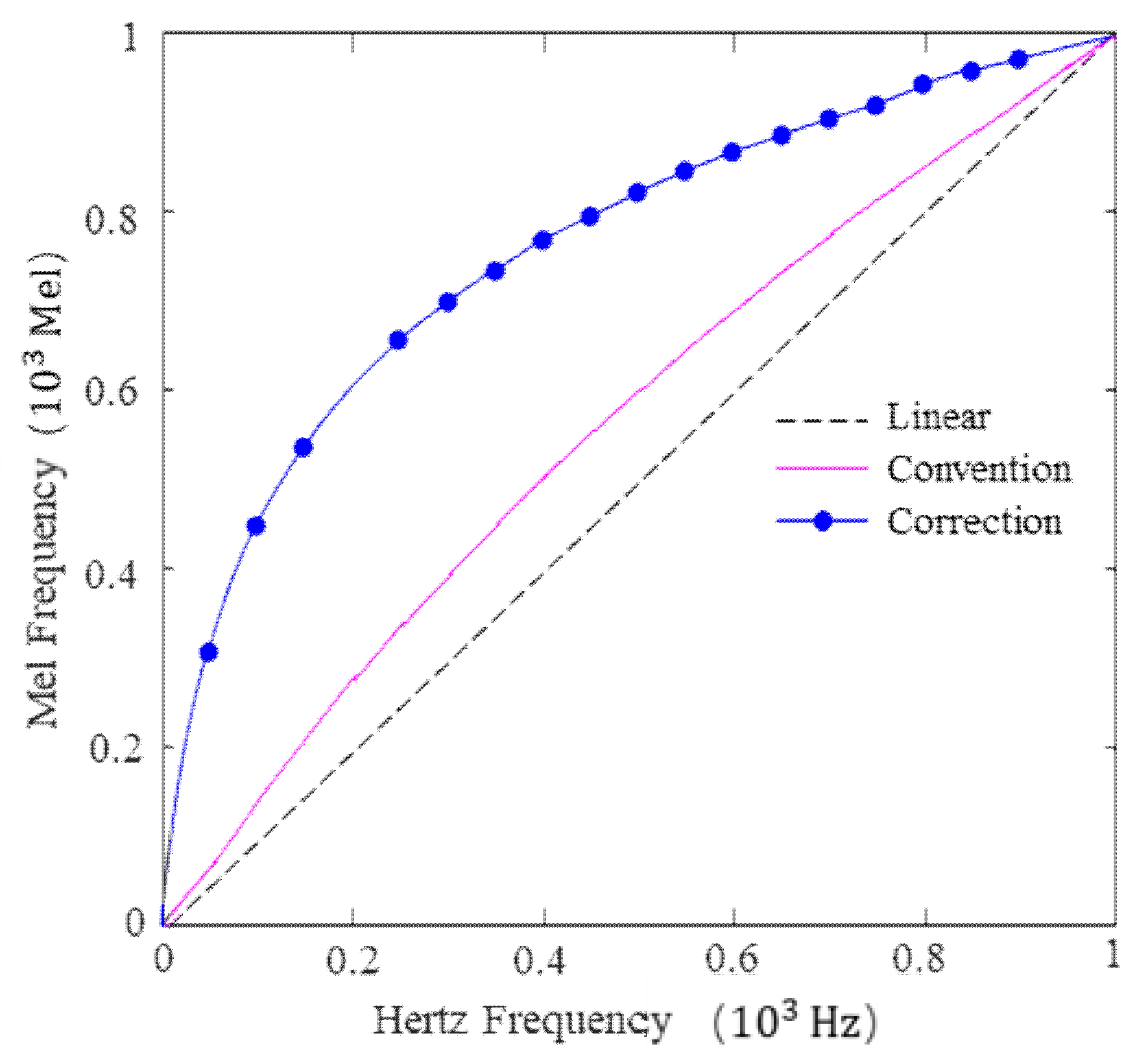
- Step 3: Preprocess mode components . To compensate for high frequency loss, each mode component is first weighed, and the weighted filter is shown in Equation (12), where ρ represents a constant (default ρ = 0.96):Then, a framing and hamming window are used successively to convert non-stationary signals into quasi-stationary signals, thereby reducing frequency leakage.
- Step 4: To carry out fast a Fourier transform (FFT). The FFT transformation is presented in Equation (13), where p represents the pth line in frequency-domain, N is the data point number of , and l refers to the lth sub-frame signal:
- Step 5: To calculate the linear spectrum energy of each frame signal. Linear spectrum energy corresponding to the lth sub-frame signal is represented in Equation (14):
- Step 6: Design a series of triangular filters named Mel filter banks, calculate the Mel-frequency spectrum energy of each frame signal, and then take the logarithm:
- Step 7: To introduce discrete cosine transform (DCT) and extract the IVMD-MFCC features. This relationship is expressed as Equation (16):where IM stands for the IVMD-MFCC feature of lth sub-frame signal, S(l, p) represents the Mel-frequency spectrum energy, and F is the number of Mel filters or features (fr = 0,1,…,F), (default F = 20).
4.3. Vector Quantization
4.4. K-Nearest Neighbor (KNN)
4.5. Outline of the Proposed Method
5. Diagnosis Results of Valve Clearance Fault
5.1. Results Analysis of the Proposed Method
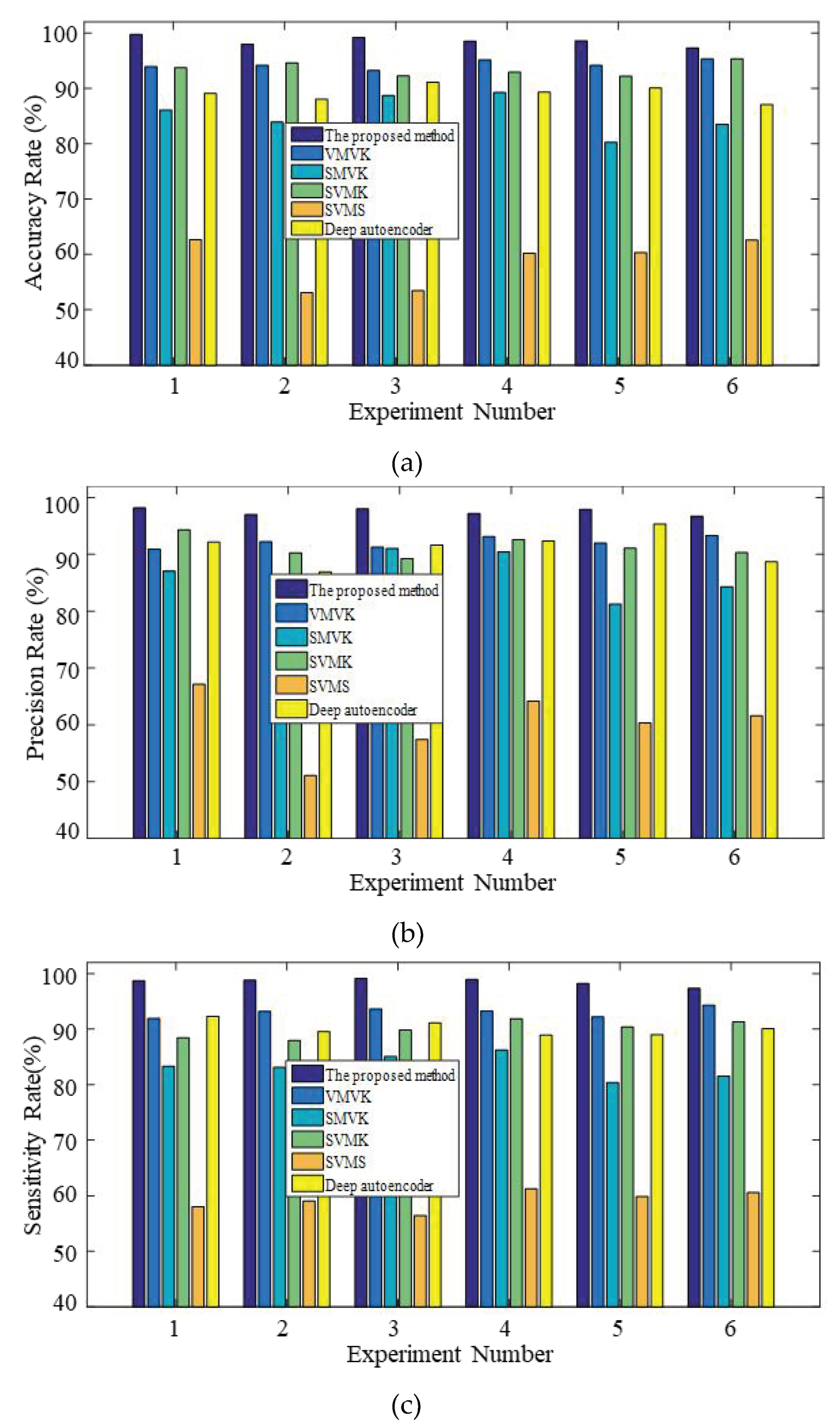
5.2. Results Analysis of Comparative Methods
6. Conclusions
Author Contributions
Funding
Conflicts of Interest
Abbreviations
| Abbreviations | ss | The ssth label of testing sample | |
| AC | Accuracy | Mel | Mel frequency |
| EEMD | Ensemble empirical mode decomposition | f | Hertz frequency |
| EVCI | Exhaust valve closing impact | Y | Fast Fourier transform of mode component |
| FFT | Fast fourier transform | t | Time |
| FI | Fire impact | E | The linear spectrum energy of pth line of each frame signal |
| FINC | Fire impact adjacent cylinder | The kth decomposed mode components | |
| IVCI | Intake valve closing impact | Central frequency | |
| IVMD-MFCC | Improved vibrational mode decomposition and Mel frequency cepstrum coefficient | , , | The corresponding Fourier transformation |
| LBG | Linde -Buzo-Gray | x(t) | Original signal |
| LDA | Linear discriminative analysis | j | Imaginary unit |
| LFE | Large clearance fault of exhaust valve | p | The pth line in frequency-domain |
| LFI | Large clearance fault of intake valve | N | The data point number of |
| LFIE | Large clearance fault of intake and exhaust valve | s | The sth data of |
| LMD | Local mean decomposition | L | the integer cycle signal length |
| Ma Tec | Maintenance technicians | M | Number of sliding windows |
| MFC | Mel frequency cepstrum coefficient | IM | IVMD-MFCC feature |
| MFCC | Mel frequency cepstrum coefficient | l | the lth sub-frame signal |
| NVC | Normal valve clearance | Rrms | Mean square root of correlation coefficient |
| PCA | Principal component analysis | d | Euclidean distance between X and Yc |
| PR | Precision | n | Number of iterations |
| IMFs | Intrinsic mode functions | J | The number of feature vector subspaces |
| ISOMap | Isometric feature mapping | ρ | A constant |
| SE | Sensitivity | F | The total number of Mel filter banks |
| SHM | Structural health monitoring | fr | The frth Mel filter bank |
| SI | Signal improvement | X | Training set of vector quantization |
| SFE | Small clearance fault of exhaust valve | Yc | Codebook of cth subspace |
| SFI | Small clearance fault of intake valve | S | Mel-frequency spectrum energy of each frame signal |
| SFIE | Small clearance fault of intake and exhaust valve | SU | Number of training set subspaces |
| SMVK | The proposed method without VMD | Tts | Training sample of KNN |
| SVMK | The proposed method without vector quantization | Wls | Label set of Tn |
| SVMS | The proposed method replacing KNN with SVM | SSS | Testing sample of KNN |
| STFT | Short time Fourier transform spectrum | Nwl | Length of sliding window |
| VMD | Variational mode decomposition | Nss | Moving step size of sliding window |
| VMVK | The proposed method without signal improvement | m | The mth data point of the sliding window |
| VQ | Vector quantization | Convergence criteria of vector quantization | The mth data point of the sliding window |
| Symbols | Total distortion of all subspaces | ||
| Convergence criteria | Ra | Correlation coefficient between (a − 1)th and ath sliding window | |
| A castigatory quadratic | TS | Number of training sample | |
| Lagrangian multiplicator operator | SS | Number of testing sample | |
| extended Lagrangian function | ts | The tsth training sample | |
| δ | Dirac distribution function | ls | The lsth label of training sample |
| τ | Noise tolerance parameter | ||
References
- Zhang, M.Q.; Zi, Y.Y.; Niu, L.K.; Xi, S.T.; Li, Y.Q. Intelligent Diagnosis of V-Type Marine Diesel Engines Based on Multifeatures Extracted from Instantaneous Crankshaft Speed. IEEE Trans. Instrum. Meas. 2019, 68, 722–740. [Google Scholar] [CrossRef]
- Zhao, X.L.; Cheng, Y.; Wang, L.M.; Ji, S.B. Real time identification of the internal combustion engine combustion parameters based on the vibration velocity signal. J. Sound Vib. 2017, 390, 205–217. [Google Scholar] [CrossRef]
- Basurko, O.C.; Uriondo, Z. Condition-based maintenance for medium speed diesel engines used in vessels in operation. Appl. Therm. Eng. 2015, 80, 404–412. [Google Scholar] [CrossRef]
- Yang, Y.S.; Ming, A.B.; Zhang, Y.Y.; Zhu, Y.S. Discriminative non-negative matrix factorization (DNMF) and its application to the fault diagnosis of diesel engine. Mech. Syst. Signal. Process. 2017, 95, 158–171. [Google Scholar] [CrossRef]
- Santos-Ruiz, I.; López-Estrada, F.R.; Puig, V.; Pérez-Pérez, E.J.; Mina-Antonio, J.D.; Valencia-Palomo, G. Diagnosis of fluid leaks in pipelines using dynamic PCA. In Proceedings of the 10th IFAC Symposium on Fault Detection, Supervision and Safety for Technical Processes SAFEPROCESS 2018, Warsaw, Poland, 29–31 August 2018; Volume 51, pp. 373–380. [Google Scholar]
- López-Estrada, F.R.; Theilliol, D.; Astorga-Zaragoza, C.M.; Ponsart, J.C.; Valencia-Palomo, G.; Camas-Anzuetoet, J. Fault diagnosis observer for descriptor Takagi-Sugeno systems. Neurocomputing 2019, 143, 48–58. [Google Scholar] [CrossRef]
- Qian, S.L.; Zhou, S.H.; Chang, W.B.; Xiao, Y.Y.; Wei, F.J. A diagnosis method for diesel engine wear fault based on grey rough set and SOM neural network. In Safety and Reliability–Safe Societies in a Changing World; Barros, A., van Gulijk, C., Haugen, S., Erik Vinnem, J., Kongsvik, T., Eds.; CRC Press: Austin, TX, USA, 2018; pp. 995–1002. [Google Scholar]
- Gómez- Peñate, S.; Valencia-Palomo, G.; López-Estrada, F.R.; Astorga-Zaragoza, C.M.; Osornio-Rios, R.A.; Santos-Ruiz, I. Sensor fault diagnosis based on a H∞ sliding mode and unknown input observer for takagi-sugeno systems with uncertain premise variables. Asian J. Control. 2019, 21, 1–15. [Google Scholar] [CrossRef]
- Cao, W.; Dong, G.N.; Chen, W.; Wu, J.Y.; Xie, Y.B. Multisensor information integration for online wear condition monitoring of diesel engines. Tribol. Int. 2015, 82, 68–77. [Google Scholar] [CrossRef]
- Geng, Z.M.; Chen, J.; Hull, J.B. Analysis of engine vibration and design of an applicable diagnosing approach. Int. J. Mech. Sci. 2003, 45, 1391–1410. [Google Scholar] [CrossRef]
- Ahmad, T.A.; Alireza, M. Fault detection of injectors in diesel engines using vibration time-frequency analysis. Appl. Acoust. 2019, 143, 48–58. [Google Scholar]
- Zeng, R.L.; Zang, R.; Ding, L.; Mei, J.M.; Zhang, L.L. Fault diagnosis of diesel engine based on genetic algorithms and dempster-shafer fusion theory. In Proceedings of the 29th Chinese Control and Decision Conference (CCDC), Chongqing, China, 28–30 May 2017. [Google Scholar]
- Zhong, J.H.; Wong, P.K.; Yang, Z.X. Fault diagnosis of rotating machinery based on multiple probabilistic classifiers. Mech. Syst. Signal. Process. 2018, 108, 99–104. [Google Scholar] [CrossRef]
- Delvecchio, S.; Bonfiglio, P.; Pompoli, F. Vibro-acoustic condition monitoring of Internal Combustion Engines: A critical review of existing techniques. Mech. Syst. Signal. Process. 2018, 99, 661–683. [Google Scholar] [CrossRef]
- Guan, Y.P.; Liang, M.; Necsulescu, D.S. Velocity synchronous bilinear distribution for planetary gearbox fault diagnosis under non-stationary condition. J. Sound Vib. 2019, 443, 212–229. [Google Scholar] [CrossRef]
- Buzzoni, M.; Mucchi, E.; Dalpiaz, G. A CWT-based methodology for piston slap experimental characterization. Mech. Syst. Signal. Process. 2017, 86, 16–28. [Google Scholar] [CrossRef]
- Hao, Y.S.; Song, L.Y.; Cui, L.L.; Wang, H.Q. A three-dimensional geometric features-based SCA algorithm for compound faults diagnosis. Measurement 2019, 134, 480–491. [Google Scholar] [CrossRef]
- Song, Y.X.; Liu, J.T.; Chu, N.; Wu, P.; Wu, D.Z. A novel demodulation method for rotating machinery based on time-frequency analysis and principal component analysis. J. Sound Vib. 2019, 442, 645–656. [Google Scholar] [CrossRef]
- Hu, X.; Peng, S.; Hwang, W.L. EMD revisited: A new understanding of the envelope and resolving the mode-mixing problem in AM-FM signals. IEEE Trans. Signal Process. 2012, 60, 1075–1086. [Google Scholar]
- Zhao, C.; Li, Z.X.; Hu, C.; Chen, S.; Wang, J.G.; Zhang, X.G. An optimized ensemble local mean decomposition method for fault detection of mechanical components. Meas. Sci. Technol. 2017, 28, 035102. [Google Scholar]
- Zvokelj, M.; Zupan, S.; Prebil, I. EEMD-based multiscale ICA method for slewing bearing fault detection and diagnosis. J. Sound Vib. 2016, 370, 394–423. [Google Scholar] [CrossRef]
- Dragomiretskiy, K.; Zosso, D. Variational mode decomposition. IEEE Trans. Signal Process. 2014, 62, 531–544. [Google Scholar] [CrossRef]
- Cai, W.N.; Yang, Z.J.; Wang, Z.J.; Wang, Y.L. A New Compound Fault Feature Extraction Method Based on Multipoint Kurtosis and Variational Mode Decomposition. Entropy 2018, 20, 521. [Google Scholar] [CrossRef]
- Huang, Y.; Lin, J.H.; Liu, Z.C.; Wu, W.Y. A modified scale-space guiding variational mode decomposition for high-speed railway bearing fault diagnosis. J. Sound Vib. 2019, 444, 216–234. [Google Scholar] [CrossRef]
- Mao, Z.W.; Jiang, Z.N.; Zhao, H.P.; Zhang, J.J. Vibration-based fault diagnosis method for conrod small-end bearing knock in internal combustion engines. Insight 2018, 60, 418–425. [Google Scholar] [CrossRef]
- Balsamo, L.; Betti, R.; Beigi, H. A structural health monitoring strategy using cepstral features. J. Sound Vib. 2014, 333, 4526–4542. [Google Scholar] [CrossRef]
- Zhang, G.; Harichandran, R.S.; Ramuhalli, P. Application of noise cancelling and damage detection algorithms in NDE of concrete bridge decks using impact signals. J. Nondestruct. Eval. 2011, 30, 259–272. [Google Scholar] [CrossRef]
- Davis, S.; Mermelstein, P. Comparison of parametric representations for monosyllabic word recognition in continuously spoken sentences. IEEE Trans. Acoust. Speech 1980, 28, 357–366. [Google Scholar] [CrossRef] [Green Version]
- Martinez, A.M.; Kak, A.C. PCA versus LDA. IEEE Trans. Pattern Anal. Mach. Intell. 2001, 23, 228–233. [Google Scholar] [CrossRef]
- Hamadache, M.; Lee, D. Principal component analysis based signal-to-noise ratio improvement for inchoate faulty signals: Application to ball bearing fault detection. Int. J. Control. Autom. Syst. 2017, 15, 506–517. [Google Scholar] [CrossRef]
- Zhang, Y.; Li, B.W.; Wang, Z.B.; Wang, W.; Wang, L. Fault diagnosis of rotating machine by isometric feature mapping. J. Mech. Sci. Technol. 2013, 27, 3215–3221. [Google Scholar] [CrossRef]
- Si, H.B.; Ng, B.L.; Rahman, M.S.; Zhang, J.Z. A novel and efficient vector quantization based CPRI compression algorithm. IEEE Trans. Veh. Technol. 2017, 66, 7061–7071. [Google Scholar] [CrossRef]
- Song, Z.Y. Application in Speech Signal Analysis and Synthesis of MTALAB; Beihang University Press: Beijing, China, 2013; pp. 16–17. [Google Scholar]
- Randall, R.B. A history of cepstrum analysis and its application to mechanical problems. Mech. Syst. Signal. Process. 2017, 97, 3–19. [Google Scholar] [CrossRef]
- Chamay, M.; Oh, S.; Kim, Y.J. Development of a diagnostic system using LPC/cepstrum analysis in machine vibration. J. Mech. Sci. Technol. 2013, 27, 2629–2636. [Google Scholar] [CrossRef]
- Volkmann, J.; Stevens, S.S.; Newman, E.B. A scale for the measurement of the psychological magnitude pitch. J. Acoust. Soc. Am. 1937, 8, 208. [Google Scholar] [CrossRef]
- Ali, Z.; Elamvazuthi, I.; Alsulaiman, M.; Muhammad, G. Detection of Voice Pathology using Fractal Dimension in a Multiresolution Analysis of Normal and Disordered Speech Signals. J. Med. Syst. 2016, 40, 20. [Google Scholar] [CrossRef] [PubMed]
- Bergstra, J.; Bardenet, R.; Bengio, Y.; Balázs, K. Algorithms for hyper-parameter optimization. In Proceedings of the 24th International Conference on Neural Information Processing Systems, Granada, Spain, 12–15 December 2011. [Google Scholar]
- Liu, Y.; Duan, L.X.; Yuan, Z.; Wang, N.; Zhao, J.P. An intelligent fault diagnosis method for reciprocating compressors based on LMD and SDAE. Sensors 2019, 19, 1041. [Google Scholar] [CrossRef] [PubMed]
- Niu, X.X.; Wang, H.C.; Hu, S.; Yang, C.L.; Wang, Y.Y. Multi-objective online optimization of a marine diesel engine using NSGA-II coupled with enhancing trained support vector machine. Appl. Therm. Eng. 2018, 137, 218–227. [Google Scholar] [CrossRef]


| Case | Intake Valve | Exhaust Valve | Number of Training Samples | Number of Testing Samples |
|---|---|---|---|---|
| Normal valve clearance (NVC) | 0.3 | 0.5 | 120 | 980 |
| Small clearance fault of intake valve (SFI) | 0.25 | 0.5 | 120 | 980 |
| Large clearance fault of intake valve (LFI) | 0.4 | 0.5 | 120 | 980 |
| Small clearance fault of exhaust valve (SFE) | 0.3 | 0.45 | 120 | 980 |
| Large clearance fault of exhaust valve (LFE) | 0.3 | 0.6 | 120 | 980 |
| Small clearance fault of intake and exhaust valve (SFIE) | 0.25 | 0.45 | 120 | 980 |
| Large clearance fault of intake and exhaust valve (LFIE) | 0.4 | 0.6 | 120 | 980 |
| Number | Speed (rpm) | Load (N·m) | Number | Speed (rpm) | Load (N·m) |
|---|---|---|---|---|---|
| 1 | 1500 | 700 | 7 | 1800 | 1600 |
| 2 | 1500 | 1000 | 8 | 2100 | 700 |
| 3 | 1500 | 1300 | 9 | 2100 | 1000 |
| 4 | 1800 | 700 | 10 | 2100 | 1300 |
| 5 | 1800 | 1000 | 11 | 2100 | 1600 |
| 6 | 1800 | 1300 | 12 | 2100 | 2200 |
| Predicted Class | |||||||||||
|---|---|---|---|---|---|---|---|---|---|---|---|
| NVC | SFI | LFI | SFE | LFE | SFIE | LFIE | AC (%) | PR (%) | SE (%) | ||
| Actual Class | NVC | 956 | 4 | 8 | 3 | 2 | 5 | 2 | 97.55 | 93.36 | |
| SFI | 22 | 958 | 0 | 0 | 0 | 0 | 0 | 97.76 | 99.58 | ||
| LFI | 42 | 0 | 938 | 0 | 0 | 0 | 0 | 95.71 | 99.15 | ||
| SFE | 0 | 0 | 0 | 980 | 0 | 0 | 0 | 100 | 99.69 | ||
| LFE | 4 | 0 | 0 | 0 | 976 | 0 | 0 | 99.59 | 99.80 | ||
| SFIE | 0 | 0 | 0 | 0 | 0 | 980 | 0 | 100 | 99.49 | ||
| LFIE | 0 | 0 | 0 | 0 | 0 | 0 | 980 | 100 | 99.80 | ||
| Overall Performance | 98.66 | 98.66 | 98.70 | ||||||||
| Predicted Class | |||||||||||
|---|---|---|---|---|---|---|---|---|---|---|---|
| NVC | SFI | LFI | SFE | LFE | SFIE | LFIE | AC (%) | PR (%) | SE (%) | ||
| Actual Class | NVC | 940 | 5 | 11 | 5 | 3 | 7 | 9 | 95.92 | 87.52 | |
| SFI | 28 | 952 | 0 | 0 | 0 | 0 | 0 | 97.14 | 94.48 | ||
| LFI | 52 | 0 | 928 | 0 | 0 | 0 | 0 | 94.70 | 98.83 | ||
| SFE | 12 | 0 | 0 | 968 | 0 | 0 | 0 | 98.78 | 99.49 | ||
| LFE | 10 | 0 | 0 | 0 | 970 | 0 | 0 | 98.98 | 99.69 | ||
| SFIE | 17 | 0 | 0 | 0 | 0 | 963 | 0 | 98.27 | 99.28 | ||
| LFIE | 15 | 0 | 0 | 0 | 0 | 0 | 965 | 98.47 | 99.08 | ||
| Overall Performance | 97.46 | 97.47 | 96.91 | ||||||||
| Number of Training/Testing Samples | Average Accuracy (%) | Average Precision (%) | Average Sensitivity (%) | Average Calculation Time (s) |
|---|---|---|---|---|
| 60/1040 | 95.71 | 93.18 | 96.12 | 52.32 |
| 120/980 | 98.54 | 97.50 | 98.50 | 55.30 |
| 180/920 | 98.86 | 97.66 | 98.17 | 65.15 |
| 240/860 | 99.72 | 98.80 | 98.35 | 80.38 |
| 300/800 | 99.70 | 99.15 | 98.30 | 100.86 |
| Methods | Average Accuracy (%) | Average Precision (%) | Average Sensitivity (%) | Average Calculation Time (s) |
|---|---|---|---|---|
| The proposed method | 98.54 | 97.50 | 98.50 | 55.30 |
| VMVK | 94.31 | 92.15 | 93.08 | 50.15 |
| SMVK | 85.27 | 86.56 | 83.25 | 40.76 |
| SVMK | 93.50 | 91.31 | 89.95 | 80.20 |
| SVMS | 58.72 | 60.30 | 59.22 | 42.38 |
| Deep autoencoder | 89.11 | 91.20 | 90.15 | 70.86 |
© 2019 by the authors. Licensee MDPI, Basel, Switzerland. This article is an open access article distributed under the terms and conditions of the Creative Commons Attribution (CC BY) license (http://creativecommons.org/licenses/by/4.0/).
Share and Cite
Zhao, H.; Zhang, J.; Jiang, Z.; Wei, D.; Zhang, X.; Mao, Z. A New Fault Diagnosis Method for a Diesel Engine Based on an Optimized Vibration Mel Frequency under Multiple Operation Conditions. Sensors 2019, 19, 2590. https://doi.org/10.3390/s19112590
Zhao H, Zhang J, Jiang Z, Wei D, Zhang X, Mao Z. A New Fault Diagnosis Method for a Diesel Engine Based on an Optimized Vibration Mel Frequency under Multiple Operation Conditions. Sensors. 2019; 19(11):2590. https://doi.org/10.3390/s19112590
Chicago/Turabian StyleZhao, Haipeng, Jinjie Zhang, Zhinong Jiang, Donghai Wei, Xudong Zhang, and Zhiwei Mao. 2019. "A New Fault Diagnosis Method for a Diesel Engine Based on an Optimized Vibration Mel Frequency under Multiple Operation Conditions" Sensors 19, no. 11: 2590. https://doi.org/10.3390/s19112590