2.1 AEM thickness surveys

All measurements presented here were performed with a towed EM instrument (EM Bird) suspended below a helicopter or fixed-wing airplane and are thus named airborne EM (AEM) surveys. The EM Bird was flown with an average speed of 80 to 120 knots at mean heights of 16 m above the ice surface (Haas et al., 2009, 2010). The instrument operated in vertical dipole mode with a signal frequency of 4060 Hz and a spacing of 2.77 m between transmitting and receiving coils (Haas et al., 2009). The sampling frequency was 10 Hz, corresponding to samples every 5 to 6 m depending on flying speed. A Riegl LD90 laser altimeter was used to measure the Bird's height above the ice surface, with a range accuracy of ±0.025 m. Positioning information was obtained with a Novatel OEM2 differential GPS with a position accuracy of 3 m (Rack et al., 2013). Details of EM ice thickness sounding are explained in the following sections.

We have carried out five surveys over the fast ice in McMurdo Sound, in November of 2009, 2011, 2013, 2016, and 2017 (Fig. 1), i.e. in the end of winter when ice thickness was near its maximum. The surveys covered several east–west-oriented profiles across the sound, as closely as possible from shore to shore, with approximate lengths of 50 km. Although the exact number of profiles differed every year due to weather restrictions, ice conditions, or technical issues, we have attempted to cover the same profiles every year and to collocate them with drill-hole measurements (Sect. 2.2). The profiles repeated most often were located at latitudes of 77^∘40^′, 77^∘43^′, 77^∘46^′, and 77^∘50^′ S, i.e. 5.5 to 7.4 km apart (Fig. 1).

EM ice thickness measurements are affected by averaging within the footprint of the instrument, which results in the underestimation of maximum pressure ridge thicknesses (e.g. Kovacs et al., 1995). However, the fast ice in McMurdo Sound is mostly undeformed and level. Over such level ice without an underlying SIPL the agreement of EM thickness estimates is within ±0.1 m of drill-hole measurements (Pfaffling et al., 2007; Haas et al., 2009). McMurdo Sound therefore presents ideal conditions for EM ice thickness measurements, and the levelness of the ice allows the application of low-pass filtering to remove occasional noise from EMI interference or episodic electronic drift that affects measurements over thick ice without losing significant information on larger scales. Here, we have applied a running-window, 300-point median filter corresponding to a width of 1.5 to 1.8 km to all data unless mentioned otherwise.

However, the accuracy of 0.1 m stated above relies on accurate calibration of the EM sensor, which is typically achieved by flying over short sections of open water (Haas et al., 2009). Unfortunately open water overflights were not possible with the helicopter surveys between 2009 and 2013, due to safety regulations. Then the calibration could only be validated over drill-hole measurements and may be less accurate than reported above. Only in 2017 were we able to use a Basler B67 airplane, permitting flights over the open water in the McMurdo Sound polynya which provided ideal calibration conditions (Fig. 1f).

2.1.3 Modelling EM responses over fast ice with a SIPL

To demonstrate the sensitivity of EM measurements to the presence of a SIPL, and to evaluate the potential of determining its thickness, we performed extensive one-dimensional forward modelling of the EM response to different SIPL thicknesses and conductivities. The I and Q components of the complex relative secondary field measured with horizontal coplanar coils over n horizontally stratified layers overlying a homogeneous half-space can be calculated as (e.g. Mundry, 1984)

$$\begin{array}{}\text{(4)}& {\displaystyle }{\displaystyle }\left(I+jQ\right)=r^{\mathrm{2}}\underset{\mathrm{0}}{\overset{\mathrm{\infty }}{\int }}{\mathit{\lambda }}^{\mathrm{2}}{R}_{\mathrm{0}}{e}^{-\mathrm{2}\mathit{\lambda }{h}_{\mathrm{0}}}{J}_{\mathrm{0}}\left(\mathit{\lambda }r\right)\mathrm{d}\mathit{\lambda }.\end{array}$$

This is a so-called Hankel transform utilizing a Bessel function of the first kind of order zero (J₀), with r being the coil spacing, h₀ the receiver and transmitter height above the ice, and λ the vertical integration constant. This equation can only be solved numerically using digital filters. Here we used the filter coefficients of Guptasarma and Singh (1997) that are, for example, implemented in a computer program by Irvin (2019). R₀ is called the transverse electric reflection coefficient and is a recursive function of signal angular frequency ω and the thickness and electromagnetic properties of individual layers (electrical conductivity σ and magnetic permeability μ₀):

$$\begin{array}{ll}{\displaystyle }& {\displaystyle }{R}_{n-\mathrm{1}}=K_{n-\mathrm{1}},\\ {\displaystyle }& {\displaystyle }{R}_{k-\mathrm{2}}=(K_{k-\mathrm{2}}+R_{k-\mathrm{1}}{u}_{k-\mathrm{1}})/(\mathrm{1}+K_{k-\mathrm{2}}{R}_{k-\mathrm{1}}{u}_{k-\mathrm{1}}),\end{array}$$

with

$$\begin{array}{ll}{\displaystyle }& {\displaystyle }{u}_k=\exp (-\mathrm{2}{h}_k{v}_k),\\ {\displaystyle }& {\displaystyle }{v}_k=({\mathit{\lambda }}^{\mathrm{2}}+j\mathit{\omega }{\mathit{\mu }}_{\mathrm{0}}{\mathit{\sigma }}_k{)}^{\mathrm{1}/\mathrm{2}},\\ {\displaystyle }& {\displaystyle }{K}_{k-\mathrm{1}}=(v_{k-\mathrm{1}}-v_k)/(v_{k-\mathrm{1}}+v_k).\end{array}$$

In these equations n is the number of layers (four in this paper: non-conductive air, sea ice and snow, SIPL, and seawater), k=1 (air), …, 4 (seawater), and $j=\sqrt{(-\mathrm{1})}$. Figure 2 shows the general design of this four-layer case and also the layer properties used for the computations which are based on the typical conditions during our surveys in McMurdo Sound.

As the EM signal is ambiguous for variable layer thicknesses and conductivities, we only calculate signal changes due to variable SIPL (layer 2) thicknesses h_sipl and conductivities σ_sipl, keeping all other parameters constant and representative of our measurements: we chose instrument height h₀=16 m, sea ice (layer 1) thickness h_i=2 m and conductivity σ_i=0 mS m⁻¹, and seawater (layer 3: infinitely deep, homogeneous half-space) conductivity σ_w=2700 mS m⁻¹. SIPL conductivity σ_sipl was varied between 0 and 2700 mS m⁻¹ in steps of 300 mS m⁻¹ to study a range of properties between the two extreme cases of negligible and maximum seawater conductivity. SIPL thickness h_sipl was varied from 0 to 20 m to also include the most extreme potential cases, such as to investigate the EM signal behaviour over potentially thick platelet layers under multiyear ice or an ice shelf. Note that we chose σ_i=0 mS m⁻¹ for simplicity, while in reality consolidated sea ice still contains some brine that can slightly raise its conductivity up to σ_i=50 mS m⁻¹ or so (Haas et al., 1997). However, those small variations have little effect on the EM retrieval of consolidated ice thickness (Haas et al., 1997; 2009).

Figure 3 shows the dependence of I and Q model curves over 2 m thick consolidated ice on variable SIPL thickness and conductivity obtained using the model of Eq. (4). As expected it can be seen that I and Q do not change with increasing SIPL thickness if the SIPL conductivity is 2700 mS m⁻¹, i.e. if the SIPL is indistinguishable from seawater. I decreases exponentially with increasing SIPL thickness, the effect becoming more pronounced as SIPL conductivity decreases. When SIPL conductivity is 0 mS m⁻¹, i.e. when the SIPL is indistinguishable from consolidated ice, the resulting curve is identical to measurements over consolidated ice only, i.e. generally following the form of Eq. (1).

In contrast, and not quite intuitively, initially Q changes little with increasing SIPL conductivity and thickness. Indeed, Q even increases slightly with increasing SIPL thickness if the SIPL conductivity is high (e.g. larger than 600 mS m⁻¹). Only for very low SIPL conductivity (e.g. below 600 mS m⁻¹) does Q decrease strongly, and for a conductivity of 0 mS m⁻¹ the curve is identical to the consolidated ice case, as for I. Note that I is generally much larger than Q and that I is more strongly dependent on SIPL thickness. Therefore the sensitivity of I to the presence, thickness, and conductivity of a SIPL is much larger than that of Q.

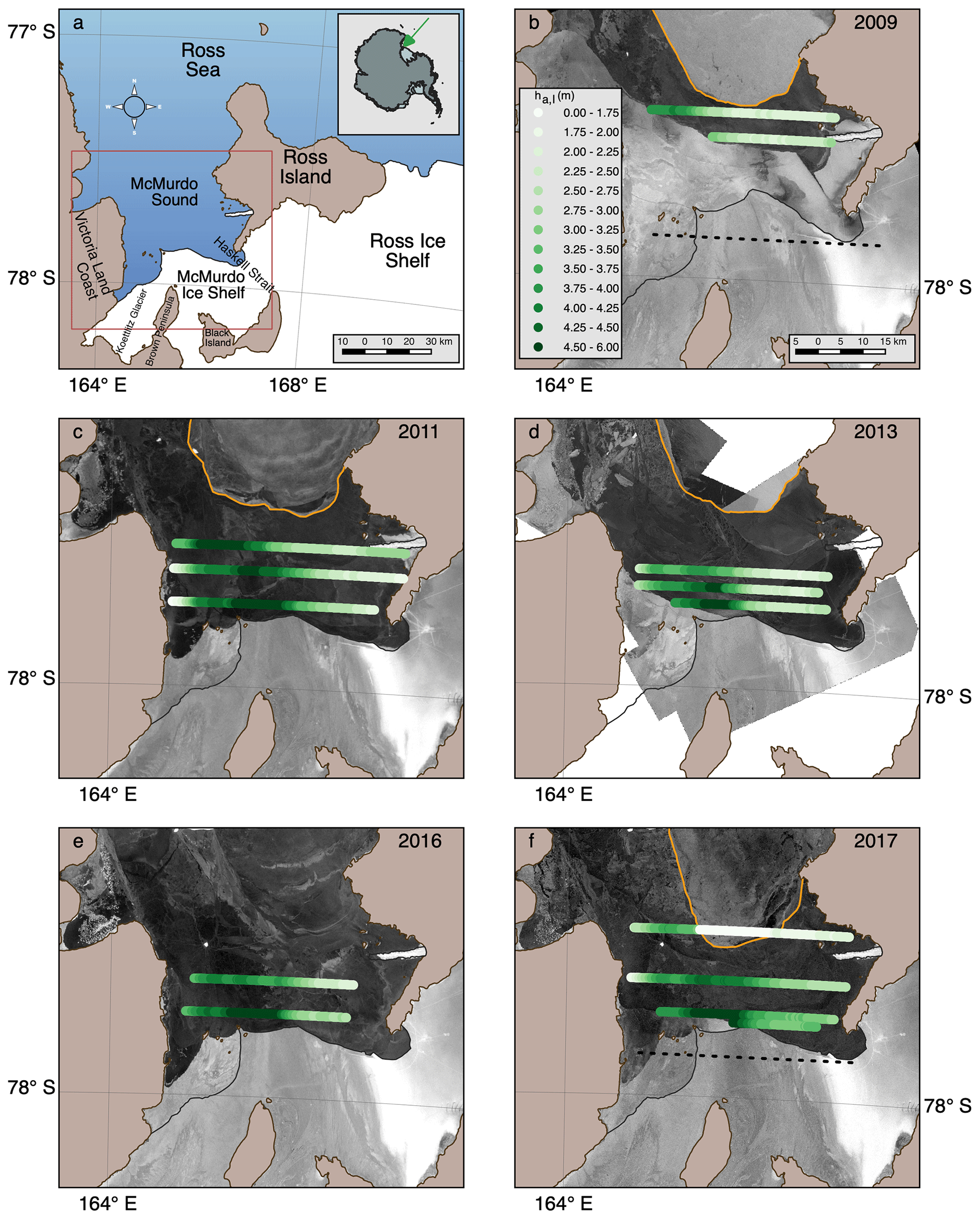
Figure 1Overview maps of the AEM surveys carried out in 2009, 2011, 2013, 2016, and 2017. (a) Regional overview and the location of McMurdo Sound (green arrow) and boundaries of satellite images (red). (b–f) Locations of east–west profiles, overlaid on synthetic-aperture radar (SAR) satellite images to show differences in general ice conditions and ice types (Brett et al., 2020; 2009/11: Envisat; 2013: TerraSAR-X; 2016/17: Sentinel-1). Colours correspond to different apparent ice thicknesses h_a,I (Sect. 2.1.2). Orange lines mark respective fast ice edges. Bright areas to the south are the McMurdo Ice Shelf. Black dashed lines in (b, f) show tracks of ice shelf thickness surveys used in Figs. 10a and 11 (Rack et al., 2013).

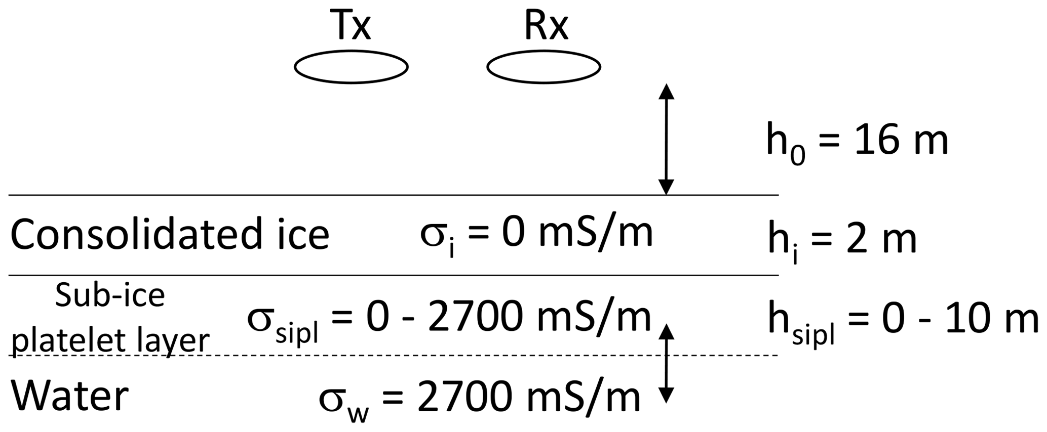
Figure 2Schematic of the four-layer forward model to compute EM responses over sea ice underlain by a SIPL with variable thickness and conductivity. Tx and Rx illustrate transmitting and receiving coils, respectively. Instrument height h₀=16 m, snow plus ice thickness h_i=2 m, and water conductivity of 2700 mS m⁻¹ are based on typical conditions during our surveys in McMurdo Sound.

Download

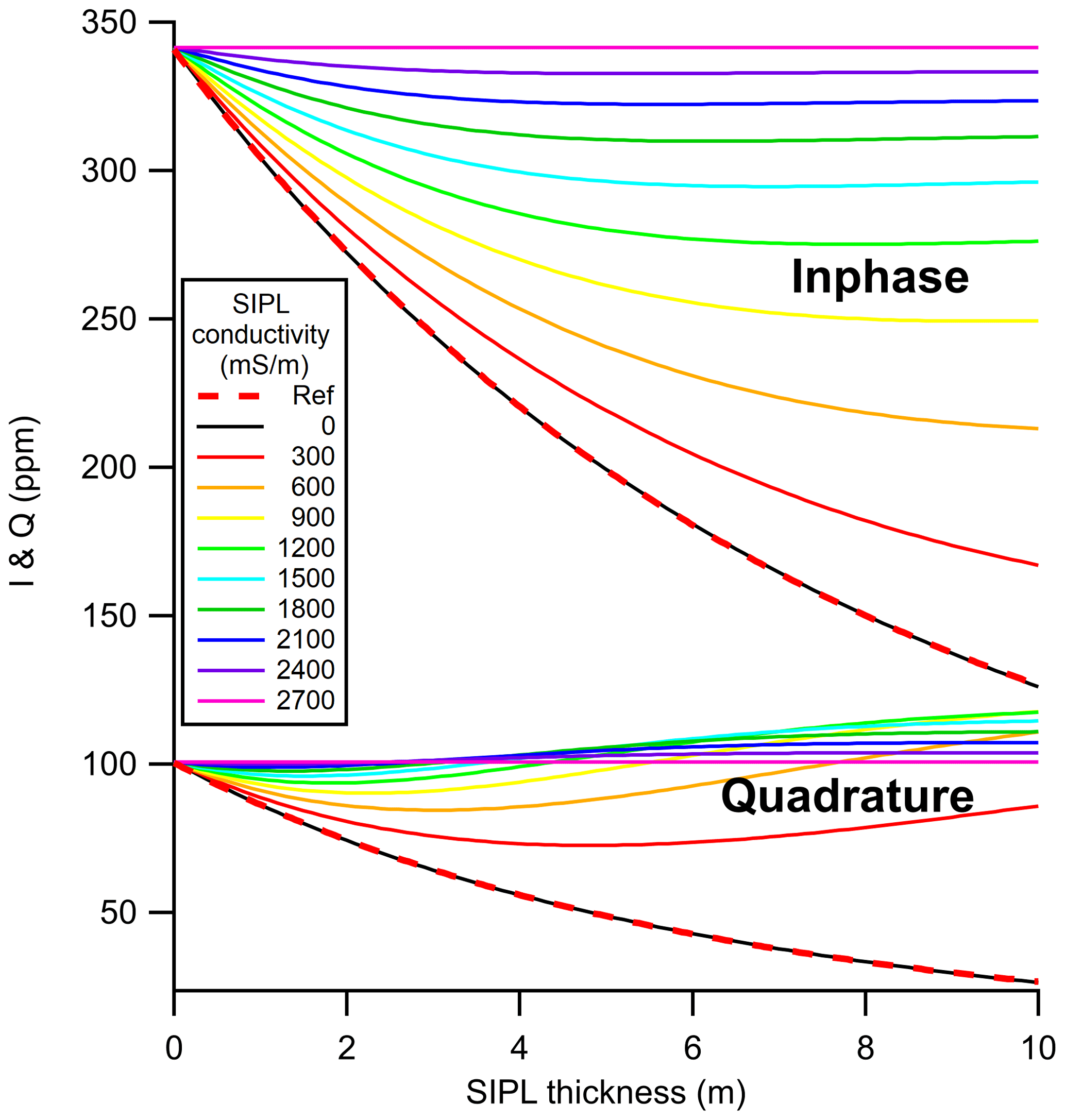
Figure 3In-phase I and quadrature Q responses to a 0 to 10 m thick SIPL under 2 m thick consolidated ice for SIPL conductivities of 0 to 2700 mS m⁻¹ computed with a three-layer EM forward model (see Fig. 2). Ref shows negative exponential curves for consolidated ice with zero conductivity used for computation of I and Q apparent thicknesses using Eq. (2b).

Download

Figure 4 shows the apparent thicknesses, h_a,I and h_a,Q, that result from applying Eq. (3a, b) to the I and Q curves in Fig. 3. Equation (3a, b) correspond to a SIPL conductivity of 0 mS m⁻¹ that would be used if the presence of an SIPL were unknown or ignored. For example, and based on the same reasoning as above, Fig. 4 shows that the apparent thicknesses agree with the total thickness h_i+h_sipl if the SIPL conductivity was zero, i.e. indistinguishable from solid ice. If the conductivity of the SIPL was indistinguishable from that of seawater (i.e. 2700 mS m⁻¹), the obtained apparent thicknesses are 2 m, i.e. the thickness of the consolidated ice only. For the in-phase component, Fig. 4a shows that apparent thicknesses for intermediate SIPL conductivities fall in between, with increasing apparent thicknesses with decreasing SIPL conductivities.

In contrast, apparent thicknesses derived from Q (Fig. 4b) are similar to the consolidated ice thickness (2 m in this case) for most SIPL conductivities. Only for SIPL conductivities below 600 mS m⁻¹ are there relatively stronger deviations, and for a SIPL conductivity of 0 mS m⁻¹ the quadrature-derived apparent thickness equals the total thickness h_i+h_sipl. In summary these results show that the in-phase signal I responds much more strongly to the presence of a SIPL than the quadrature Q.

Note that most in-phase curves level out for large SIPL thicknesses, the effect being exacerbated for higher SIPL conductivities (Fig. 3). This is due to the limited penetration depth of EM fields in highly conductive media. Accordingly the corresponding derived apparent conductivities level out with increasing SIPL thickness as well and are insensitive to further increases in SIPL thickness (Fig. 4a). In practice this means that the EM in-phase signals are only sensitive to SIPL thickness changes up to a certain SIPL thickness and that the sensitivity decreases with increasing SIPL thickness and conductivity. In contrast, while Q is relatively insensitive to the presence and thickness of a SIPL for SIPL conductivities above 600 mS m⁻¹, responses are non-monotonic for low SIPL conductivities and possess local minima at varying SIPL thicknesses. As a result, apparent thicknesses derived from Q possess local maxima at variable SIPL thicknesses.

2.2 Drill-hole validation measurements

At 55 sites over all 5 years of observation, drill-hole measurements were performed under the flight tracks of the EM Bird to measure the thickness of snow, sea ice, and the SIPL, and the freeboard of the ice. The protocol at each drill site has been described in Price et al. (2014) and Hughes et al. (2014). At each site, five measurements were made at the centre and corners of a 30 m wide “cross”. Sea ice thickness and the depth of the bottom of the sub-ice platelet layer were measured with a classical T-bar at the end of a tape measure lowered through the ice and pulled up until resistance was felt (Haas and Druckenmiller, 2009; Gough et al., 2012). This is an established method in the absence of a sub-ice platelet layer, with ice thickness accuracies of 2 to 5 cm. However, the bottom of the unconsolidated sub-ice platelet layer is often fragile and may be gradual, such that pull resistance may only increase gradually and may be difficult to feel (Gough et al., 2012). This is further complicated by the frequent presence of ice platelets inside the drill hole causing additional resistance and impeding detection of the water level within the hole. Ice crystals may be jammed between the T-anchor and the bottom of the consolidated ice, hampering the accurate determination of sea ice thickness. Following Price et al. (2014), we assume typical relative errors (1 standard deviation) for the drill-hole sea ice and sub-ice platelet layer thicknesses to be ±2 % and ±5 % to 30 %, respectively. Snow thickness was measured on the cross lines at 0.5 m intervals using a ruler (2009, 2011, and 2013) or a Magnaprobe (2016 and 2017; Sturm and Holmgren, 2018). Throughout this paper we have added snow and ice thickness to comprise total consolidated ice thickness h_i.

3.1 Apparent ice thicknesses in McMurdo Sound

The SAR images in Fig. 1b–f show that the fast ice in McMurdo Sound can be quite variable, with regard to both the location of the ice edge and the types of first-year ice that are present (Brett et al., 2020). Due to break-up events during the winter there can be refrozen leads with younger and thinner ice, or larger areas of thinner ice, as can for example be seen in 2013 in the northeast of the panel. These variable ice conditions result in variable thickness profiles that are indistinguishable from small undulations due to instrument drift. The SAR images also show the presence of multiyear landfast ice in some years, in particular in 2009. The multiyear ice is much thicker than the first-year ice, and we have few drill-hole measurements there. Therefore, results over multiyear ice are not included here.

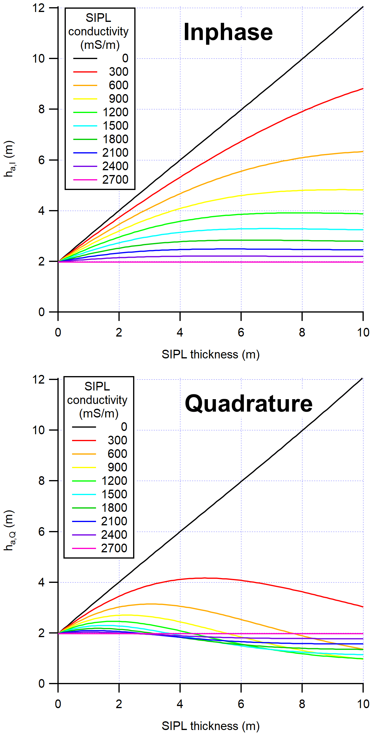
Figure 4Apparent thicknesses resulting from applying simple negative-exponential equations like in Eq. (3a, b) to the I and Q curves in Fig. 3.

Download

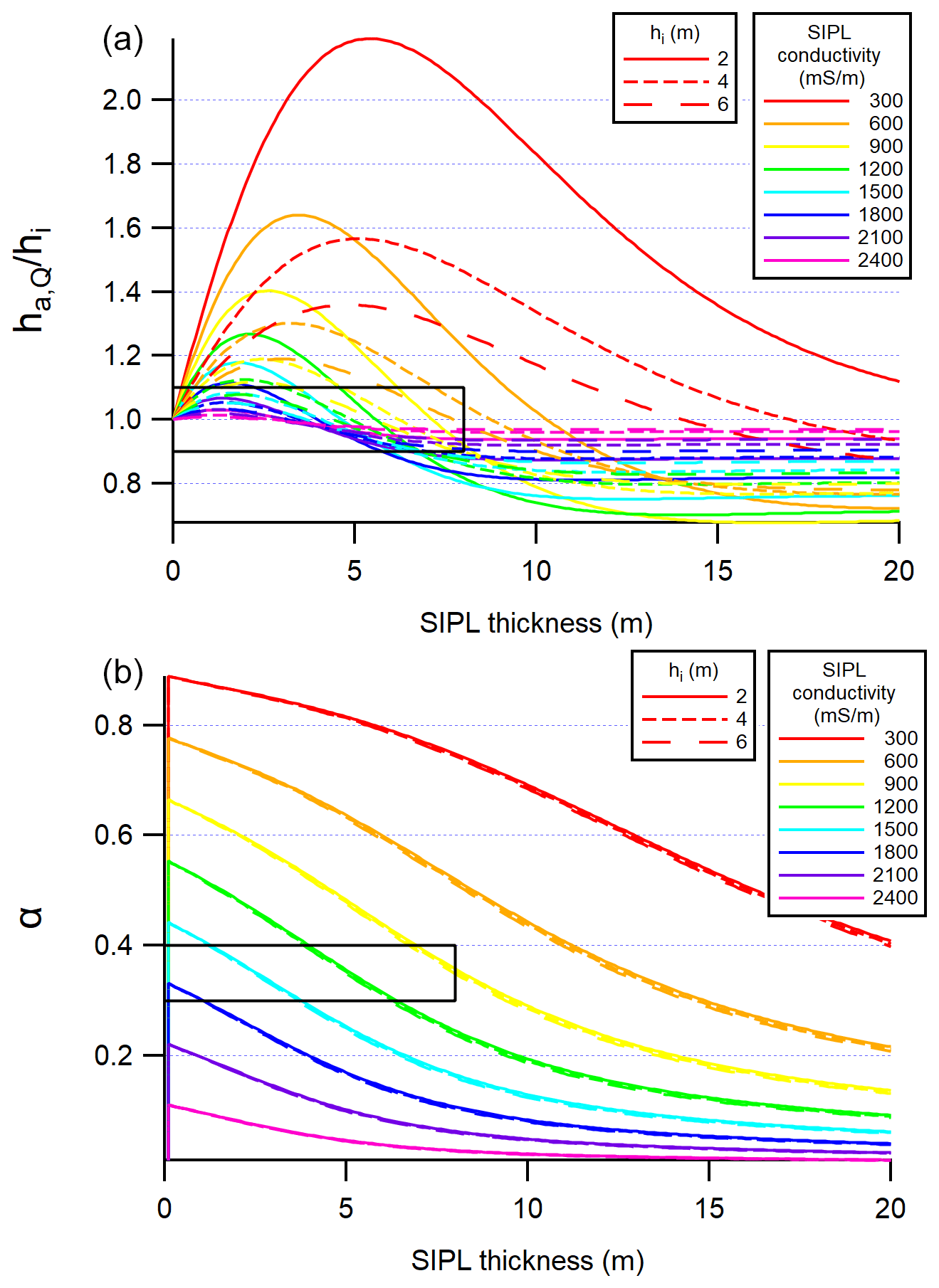
Figure 5Ratio of $h_{\text{a},Q}/h_{\mathrm{i}}$ (a; see Eq. 5a) and $\mathit{\alpha }=(h_{\text{a},I}-h_{\mathrm{i}})/h_{\text{sipl}}$ (b; see Eq. 5c) vs. SIPL thickness, at different consolidated ice thicknesses h_i between 2 and 6 m and different SIPL conductivities between 300 and 2400 mS m⁻¹. Curves follow from curves in Figs. 3 and 4. Black boxes show the range of $h_{\text{a},Q}/h_{\mathrm{i}}$ and α values resulting from the calibration (Sect. 3.2).

Download

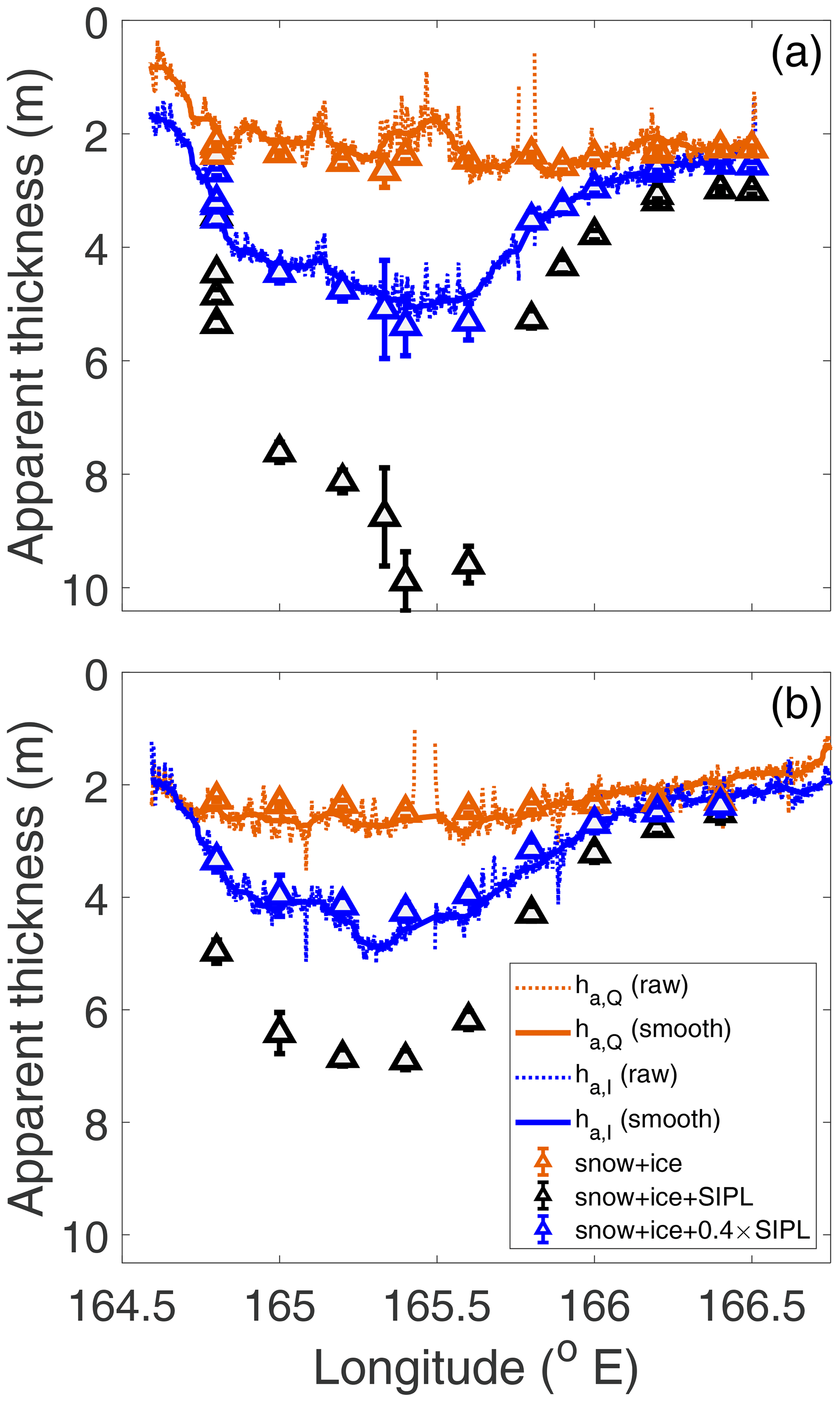
Figure 6Apparent AEM thicknesses h_a,Q (orange lines) and h_a,I (blue lines) along E–W profiles at (a) 77^∘50^′ S and (b) 77^∘46^′ S in November 2011, approximately 3 and 11 km from front of McMurdo Ice Shelf, respectively. Dotted lines are raw data, while solid lines are filtered with a 300-point median filter. Triangles show mean and standard deviation of drill-hole measurements at calibration points. Consolidated ice (snow plus ice; orange), consolidated ice plus SIPL thickness (black), and consolidated ice plus (α=0.4) × SIPL thickness (blue; Eq. 5c).

Download

Figures 1b–f also show the apparent thickness h_a,I determined from the in-phase component along the profiles. In general it can be seen that h_a,I ranges between 2.0 and 2.5 m, in the eastern side of the sound, in good agreement with other studies (Price et al., 2014, Brett et al., 2020) and with our drill-hole measurements (see below). On the western side of the sound much thicker ice, up to 6 m in apparent thickness, can be seen. The regional distribution and thickness of this thick ice coincides with our general knowledge of the distribution of the ISW plume and the SIPL in the region (Dempsey et al., 2010; Langhorne et al., 2015). In particular, the data show that apparent ice thicknesses are much larger near the ice shelf than farther north, in agreement with the fact that the ISW plume emerges from the ice shelf and then spreads north. However, the obtained apparent thicknesses are much smaller than what is known from drill-hole measurements, when SIPL thickness is taken into account. These results confirm the results of our modelling study and demonstrate that the in-phase measurements are sensitive to the presence and thickness of a SIPL.

In general, apparent thicknesses h_a,Q derived from the quadrature measurements show much less variability. We will present them below where we show the derived consolidated ice thicknesses (Sect. 3.2, Fig. 6).

Table 1Summary of drill-hole calibration results showing the number of drill-hole measurements N, derived scaling factor α (Eq. 5c), SIPL conductivity σ_SIPL, and solid fraction β. Data from several years with similar behaviour were pooled to increase the number of data points for more reliable fits.

Download Print Version | Download XLSX

Figure 7Scatter plot of EM derived vs. drill-hole consolidated ice thickness (h_i; filled symbols) and total thickness (h_i+h_sipl; open symbols), with symbol colour denoting year of measurement. Total thickness (h_i+h_silp) was calculated with α=0.4 (best fit value 0.40±0.07, N=46) for 2009, 2011, and 2017 and α=0.3 for 2013 and 2016 (best fit value 0.30±0.15, N=9); see Table 1. Error bars show ice thickness variability at each calibration location (five drill holes) or within the approximate EM footprint (the latter are too small to be visible at the scale of the graph). The black line is 1:1. N=9 for 2009, N=26 for 2011, N=5 for 2013, N=4 for 2016, and N=11 for 2017; thus total N=55.

Download

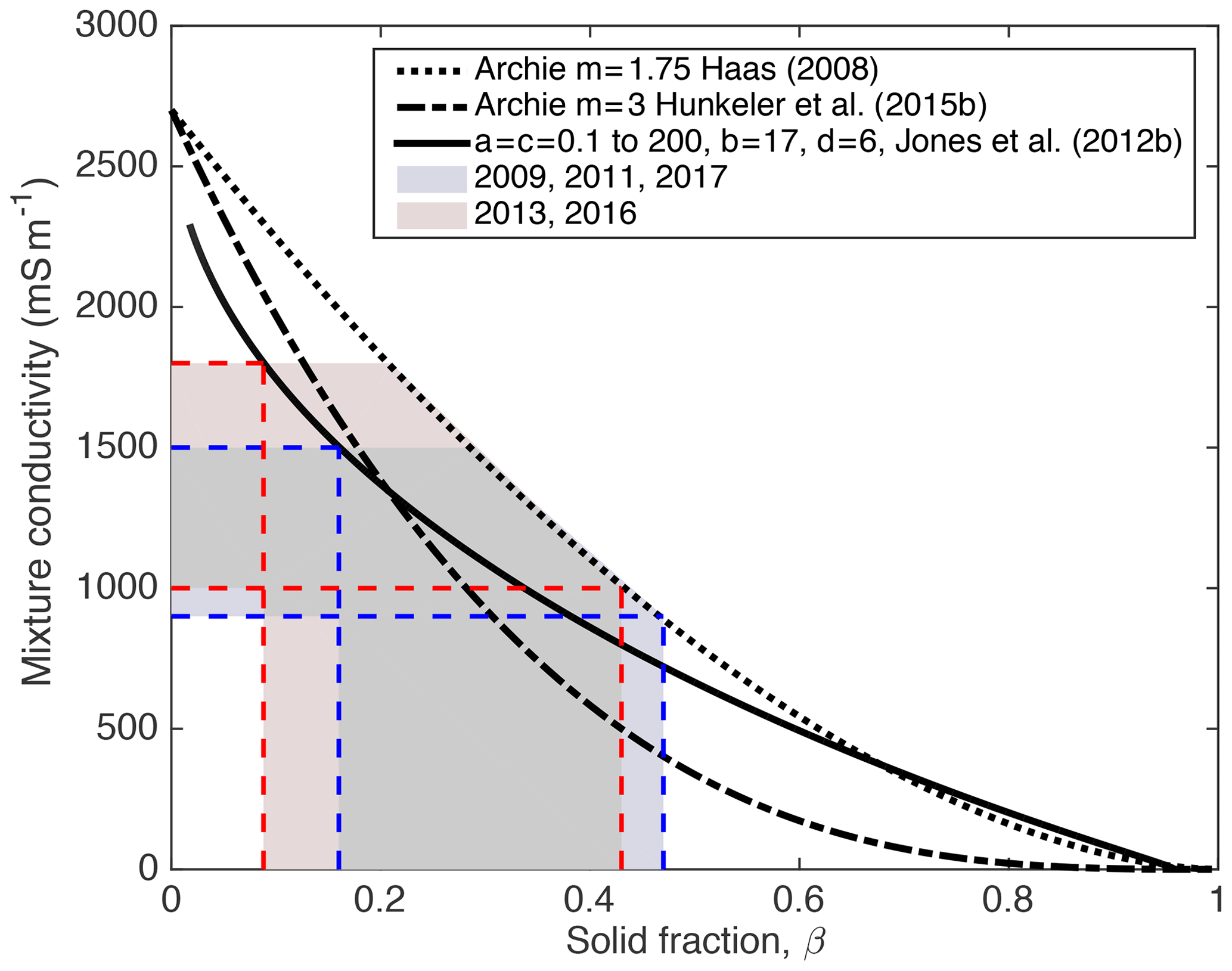
Figure 8Conductivity vs. solid fraction for porous media according to theories by Archie (1942) with different cementation factors m=1.75 and 3 and Jones et al. (2012b; black curves). Coloured areas show the range of SIPL conductivities derived from comparison of drill-hole and EM SIPL thicknesses (Fig. 5b, Table 1) and resulting solid fractions according to the different theories.

Download

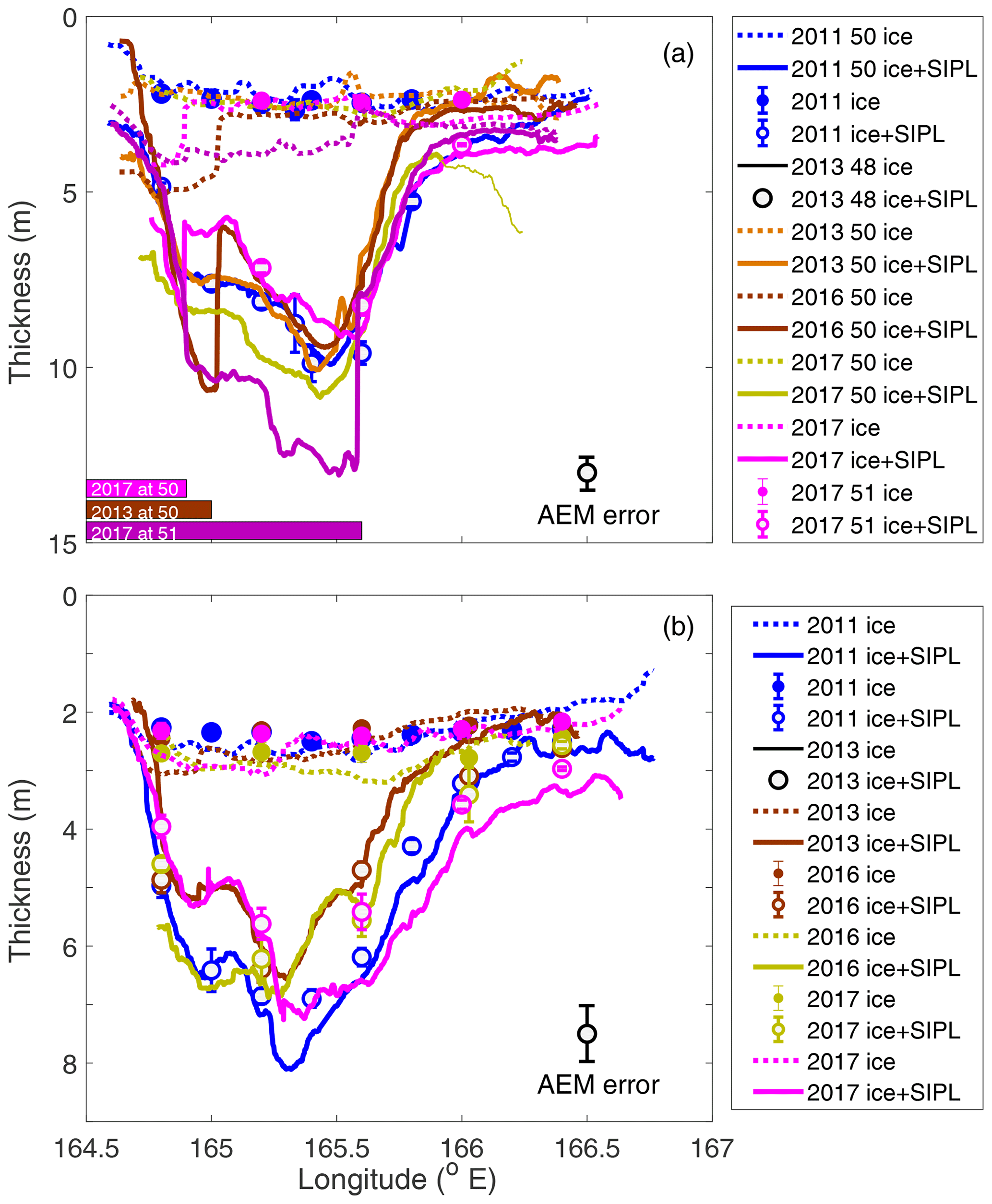
Figure 9Interannual variability of AEM-derived and drill-hole-consolidated ice h_i (stippled lines and filled symbols) and total thickness h_i+h_sipl (solid lines and open symbols) along E–W transects at similar latitude (median filtered). (a) Transects at approximately 77^∘48^′ to 77^∘51^′ S in November 2011, 2013, 2016, and 2017, approximately 3 to 5 km from the McMurdo Ice Shelf front. Horizontal bars indicate very thick MY ice present in the west along part of the profiles in 2013 and 2017. (b) Transect at approximately 77^∘46^′ S in November 2011, 2013, 2016, and 2017, approximately 11 km from McMurdo Ice Shelf front. Note different y axis scales, i.e. thicker SIPL farther south. The data reduction model uncertainty in AEM total thicknesses (snow + ice + SIPL) is shown.

Download

3.2 Calibration of consolidated ice and SIPL thickness

The behaviour of h_a,Q and h_a,I can be seen much better when vertical cross sections of individual profiles are plotted. This is shown in Fig. 6 for one profile near the ice shelf edge (Fig. 6a) and one farther north (Fig. 6b). The figure also shows drill-hole data for comparison. Note that here and in Fig. 9 we plotted thickness downwards to illustrate more intuitively the bottom of the consolidated ice and SIPL. It can be seen that h_a,Q and h_a,I agree with each other quite well in the east (right) and show an ice thickness of approximately 2.0 to 2.5 m, in agreement with the consolidated ice thickness in that region. However, farther west (left), in the region of the ISW plume and thicker SIPL, the curves deviate from each other. While h_a,Q changes relatively little, h_a,I increases strongly. The curves join again in the farthest west, where the ISW plume is known to vanish (Robinson et al., 2014). While both curves follow the expected behaviour resulting from the model results well (Sect. 2.1.3), and while h_a,Q is in reasonable agreement with the drill-hole measurements of consolidated ice thickness h_i, h_a,I strongly underestimates total ice thickness h_i+h_sipl. Therefore, according to Eq. (5b), the drill-hole measurements of SIPL thickness can be multiplied by a factor of α=0.4 for best agreement with the in-phase AEM measurements. Note that this behaviour and value for α are also in good agreement with the model results and with the range of α values predicted by Fig. 5b.

The good agreement between h_a,Q and h_i from the drill-hole data strongly supports our approach of using h_a,Q as the best estimate for h_i (Eq. 5a). This approach will be evaluated below (Fig. 7). In order to determine the best values for α, we have fit the drill-hole-measured ice and SIPL thicknesses against ($h_{\text{a},I}-h_{\text{a},Q})$ measured by the EM Bird at the same sites. These values for α are summarized in Table 1. For first-year, land-fast sea ice in 2009, 2011, and 2017, there are N=46 coincident measurements and they yield a best fit value of $\mathit{\alpha }=\mathrm{0.40}\pm \mathrm{0.07}.$ A SIPL factor of α=0.4 has been used for those years henceforth. Fewer drill-hole measurements were available in 2013 and 2016 (N=9 in total), resulting in a best fit of $\mathit{\alpha }=\mathrm{0.30}\pm \mathrm{0.15}.$ We therefore use an SIPL scaling factor of α=0.3 for 2013 and 2016 from here on.

With these α values we can then convert all in-phase and quadrature measurements into total consolidated ice plus SIPL thickness. Figure 7 shows a scatter plot of thicknesses thus derived vs. total drill-hole thicknesses. It demonstrates that EM-derived and drill-hole thicknesses agree very well, with a best fit line of slope 1.00±0.05 and intercept 0.0±0.2 (95 % confidence intervals) and root-mean-square error of 0.47 m. Based on this and the discussion of Fig. 5 above we also estimate that the systematic error associated with the uncertainty in the simplified processing of the h_a,Q and h_a,I data and the choice of α yields a data reduction model uncertainty of ±0.5 m.

3.3 SIPL conductivity and solid fraction

The SIPL scaling factors, α, are highly sensitive to SIPL conductivity and thickness (Fig. 5b). However, with known α and SIPL thicknesses from the drill-hole calibrations in Sect. 3.2 (Table 1), we can narrow down the range of possible SIPL conductivities, in particular as the range of SIPL thicknesses only extends between 0 and 8 m. The corresponding region of α values and SIPL thicknesses has been marked in Fig. 5b. It can be seen that most curves within this region have conductivities between 900 and 1800 mS m⁻¹. The range of conductivities resulting from different α in the different years is listed in Table 1.

In order to relate the conductivities to a solid fraction within the SIPL, we need a model of electrical conductivity, Archie's law being the best known (Archie, 1942). Figure 8 shows the horizontal conductivity for Archie's law with tortuosity factor and saturation exponent set to 1 (e.g. Kovacs and Morey, 1986) and cementation factor m=1.75 (Haas et al., 1997) and m=3 (Hunkeler et al., 2015b), as the solid fraction is increased from 0 to 1. For sea ice specifically, Jones et al. (2012a) have used a simple conductivity model (Jones et al., 2012b) to derive parameters for an ice/brine “unit cell”. Each unit cell consists of a single, isolated, cubical brine pocket with sides of relative dimension d (unitless) and three connected channels in perpendicular directions (two horizontal and one vertical direction), each with relative dimensions $c\times a\times b$ (also unitless). Jones et al. (2012b) found that the relative dimensions that fit the observed in situ DC horizontal and vertical resistivities depend not only on sea ice temperature but also on structure. In particular, for Antarctic incorporated platelet ice at −5 ^∘C, the shape of the inclusions has relative brine pocket dimensions a≈1, b≈17, c≈0.6, and d≈6 (see Jones et al., 2012a, for details). In addition, Jones et al. (2012b) have shown for Arctic first-year sea ice that there is a dramatic change in these parameters with temperature, with a, c, and d becoming relatively larger, while b drops. This behaviour would also be expected in incorporated platelet ice. We shall therefore assume that the shape of the inclusions in the SIPL is similar to that of incorporated platelet ice (as observed by Jones et al., 2012a) but that brine inclusion and void dimensions are very much larger because they are very close to the freezing point. Consequently, we calculate the relationship between solid fraction and conductivity from Jones et al. (2012b), by varying a and c, while keeping b and d constant and hence changing the solid and liquid content of the SIPL (see Fig. 8).

From these curves, and the conductivities derived from the comparison of EM and drill-hole SIPL thicknesses (Fig. 5b, Table 1), we can estimate the corresponding solid fraction of the SIPL, with data in Fig. 8 grouped into two sets for the range of conductivities for α=0.4 in blue (2009, 2011, 2017) and α=0.3 in red (2013, 2016). Thus the airborne measurements imply that the range of solid fractions in the SIPL lies between 0.1 and 0.5, but values are lower in 2013 and 2016 than in 2009, 2011, and 2017 (see Table 1 and Fig. 8). We shall discuss this interannual variability in Sect. 3.4.1.

3.4 Spatial and interannual variability of the SIPL

3.5 Evidence of persistent, recurring SIPL pattern

Close inspection of the thickness data in all years and at all latitudes reveals the presence of persistent, recurring local maxima or clear shoulders in the thickness profiles. Typical examples that were identified are illustrated by A and B in the repeated profiles along transect 77^∘46^′ S in 2011, 2013, 2016, and 2017 in Fig. 10a. Figure 10b shows that these maxima are also present in a series of profiles at increasing latitude or decreasing distance from the front of the McMurdo Ice Shelf. While Fig. 10a also shows the typical interannual variability of up to 2 m in SIPL thickness already seen in Fig. 9, Fig. 10b nicely demonstrates the decreasing SIPL thickness with increasing distance from the ice shelf already indicated by the differences between Fig. 9a and b.

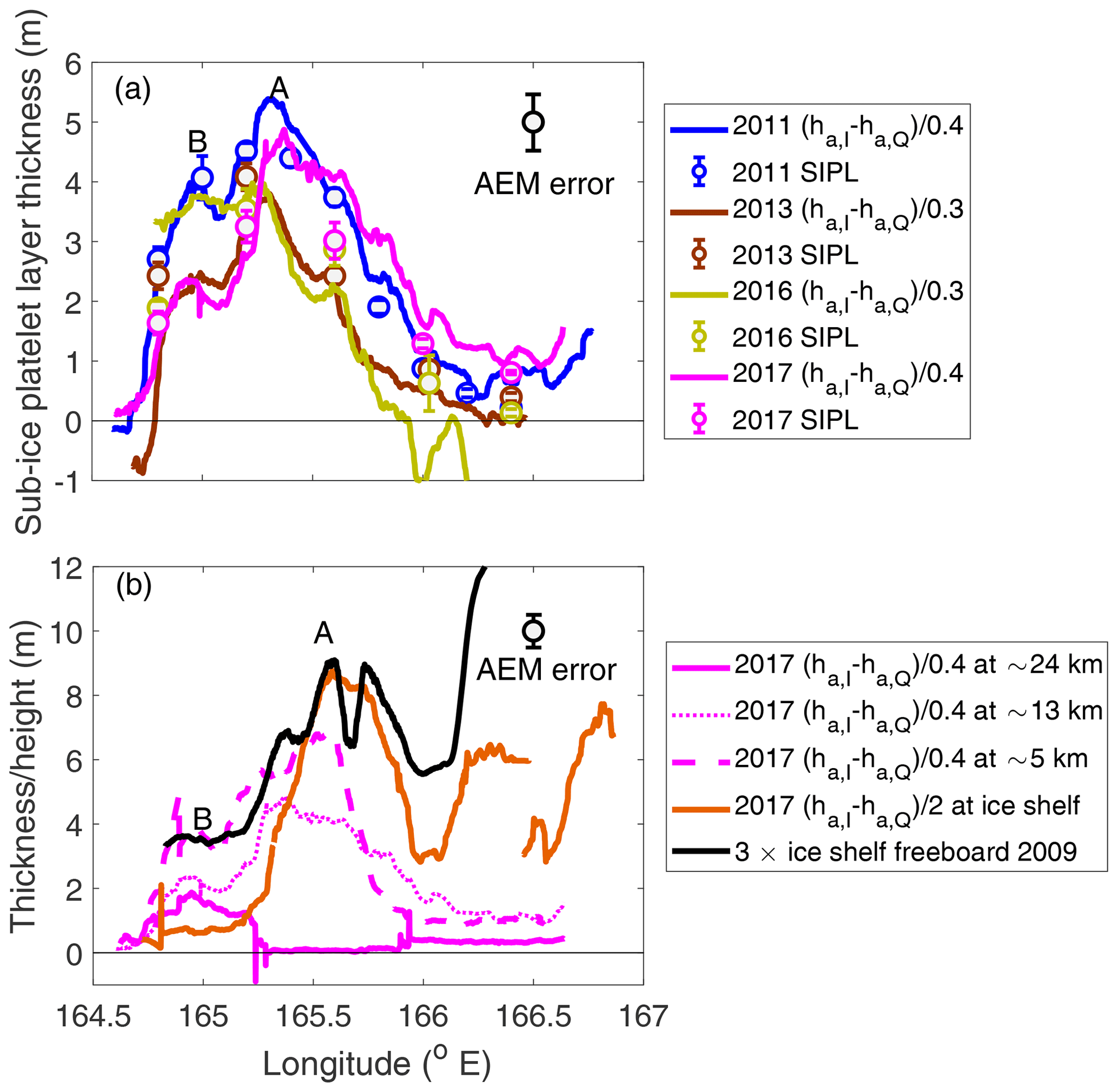
Figure 10(a) SIPL thickness along 77^∘46^′ S in 2011, 2013, 2016, and 2017, approximately 11 km from McMurdo Ice Shelf front. Recurring local maxima or shoulders in thickness are identified at A and B. (b) SIPL thickness profiles in November 2017 at different distances from McMurdo Ice Shelf front (pink lines), at approximately 24 km (solid), 13 km (dotted), and 5 km (dashed). The figure also shows uncalibrated, scaled SIPL thickness beneath the ice shelf in 2017 (brown) and scaled ice shelf freeboard in 2009 (black; from Rack et al., 2013), at 77^∘55^′ S. The ice shelf data are smoothed by a moving-average filter of window size 50. Local thickness maxima are identified at A and B. The data reduction model uncertainty in AEM total thicknesses (snow + ice + SIPL) is shown.

Download

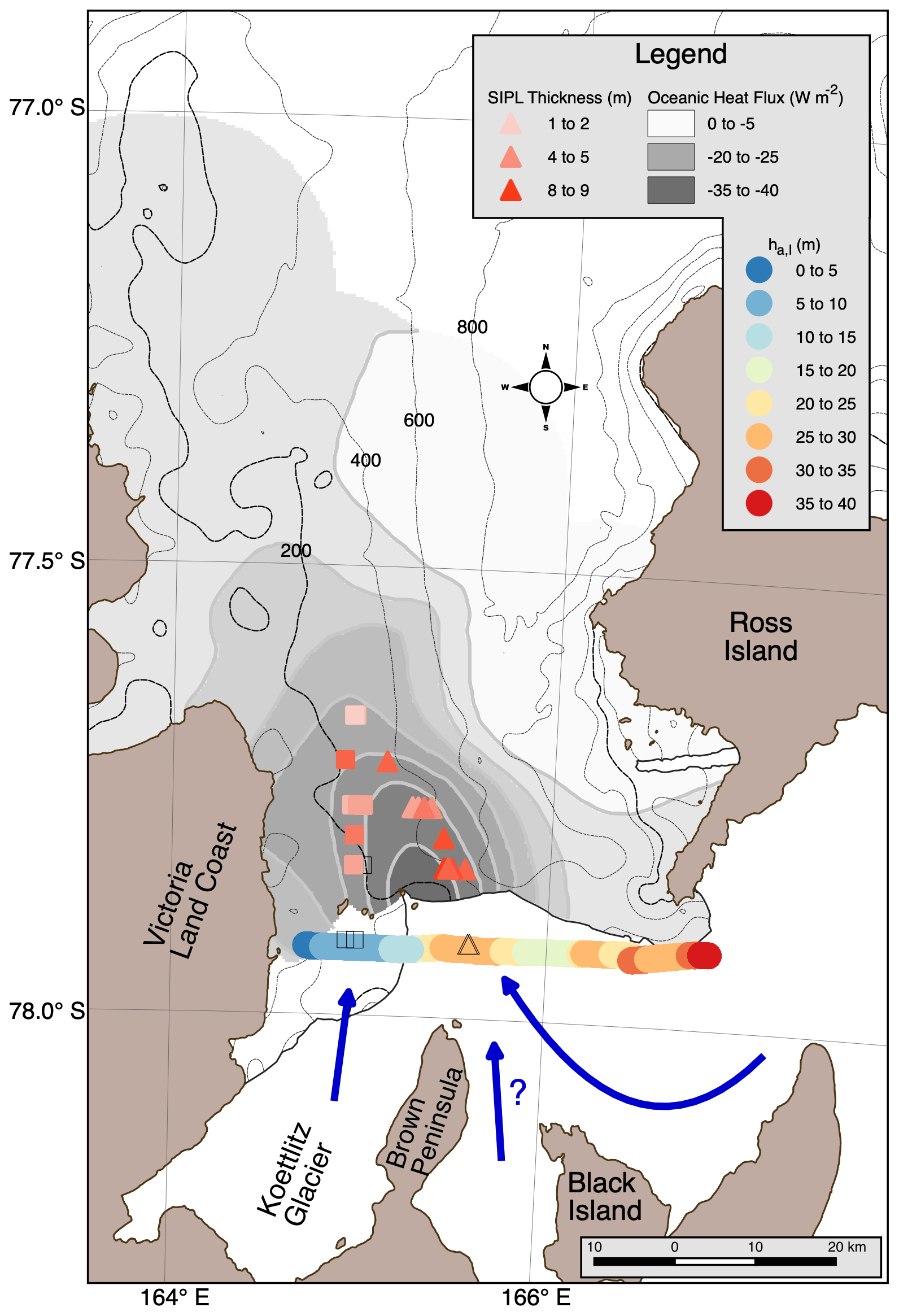
Figure 11Bathymetric map of McMurdo Sound showing the location of local maxima in SIPL thickness, with peak A as triangles and B as squares for all years 2009, 2011, 2013, 2016, and 2017. The magnitudes of the local maxima are coloured proportionally to the thickness of the peak, with darker orange for thicker average SIPL. Open symbols denote peaks whose absolute thicknesses were uncertain. Coloured horizontal line shows ice shelf h_a,I profile flown in 2017 with locations of corresponding A and B peaks identified. Contours in grey are proportional to negative ocean heat flux from Langhorne et al. (2015). Blue arrows indicate possible paths of surface ISW (based on Robinson et al., 2014).

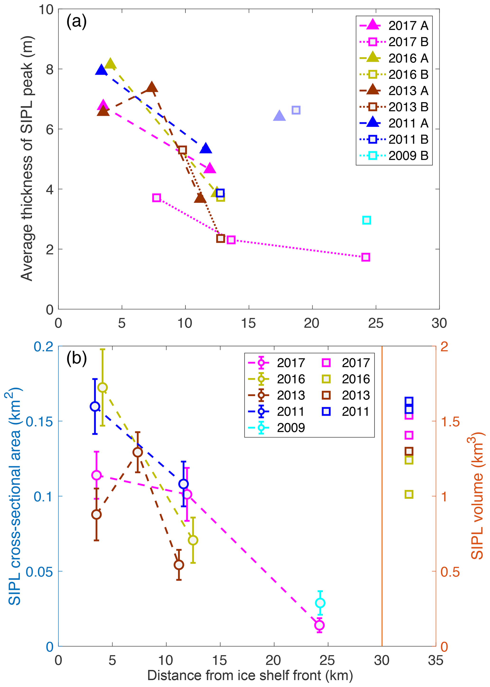
Figure 12(a) SIPL thickness of peaks A and B (averaged over 0.1^∘ of longitude) vs. distance from ice shelf front for all years 2009, 2011, 2013, 2016, and 2017 (see Fig. 11). (b) East–west cross-sectional area through the SIPL region (defined as greater than 1 m thickness). Simultaneous SIPL volumes over a 675 km² area in the central McMurdo Sound from Brett et al. (2020) are shown on the right (squares). Error bars assume a ±0.5 m data reduction model uncertainty in EM SIPL measurements (Sect. 3.2).

Download

For comparison, Fig. 10b also includes data from AEM and laser altimeter surveys of the McMurdo Ice Shelf near its front at 77^∘55^′ S (see ice shelf locations in Fig. 11) in November 2009 and 2017. It shows the ice freeboard in 2009 from Rack et al. (2013) and an uncalibrated measure of the SIPL thickness beneath the ice shelf. The latter was derived from the difference between in-phase and quadrature apparent thicknesses, $h_{\text{a},I}-h_{\text{a},Q}$, but no scaling was applied. Note that the ratio between h_a,Q and h_i and scaling factor α (Eqs. 5) under the 20 to more than 50 m thick ice shelf could be quite different than under 2 m thick sea ice and that no calibration measurements were available.

Figure 10b shows that the locations of the local maxima in SIPL thickness under the ice shelf in 2017 coincide very well with the ice shelf freeboard of Rack et al. (2013) in 2009. This could be due to preferential accretion of marine ice in those locations or due to the increased buoyancy from the SIPL under the ice shelf (Rack et al., 2013). Even more importantly, the locations of the SIPL thickness maxima under the ice shelf coincide approximately with the locations of SIPL thickness maxima under the fast ice to the north, providing evidence that the structure of the SIPL under the fast ice is directly linked to the geometry of the ISW outflow from under the ice shelf.

The local maxima A and B illustrated in Fig. 10 can be visually identified in some transects from all years 2009, 2011, 2013, 2016, and 2017 and their positions are shown in regional context on the map in Fig. 11. The peaks clearly originate under the ice shelf and propagate beneath the sea ice, carried northward by the ISW plume. The thickest peak A appears to be carried westward, as is also visible in Fig. 10. The westward displacement of this peak may be supported by the Coriolis force acting on the northward-flowing ISW (Robinson et al., 2014), as suggested by the modelling of Cheng et al. (2019) and Holland and Feltham (2005). Peak B is farther west and appears to originate from under the ice shelf near the Koettlitz glacier. Its course is more northerly as it may be constrained by the 200 m isobath. While the ice shelf thickness measurements near the front are uncalibrated, they are generally in agreement with thicknesses from 1960–1984 (McCrae, 1984) and from 2015 (Campbell et al., 2017).

Finally, Fig. 12a shows the thickness of peaks A and B from Fig. 11 vs. latitude. Thicknesses were averaged over a width 0.1^∘ of longitude centred on the peak location to be statistically more representative. Although quite noisy, the figure shows that peak A is generally larger than peak B, and that both are decreasing with distance from the ice shelf front. Peak A decreases from a maximum SIPL thickness of 8 m approximately 3 km from the front to less than 3 m at 24 km, i.e. over a distance of 21 km. The relatively large scatter of up to 2 m at single locations is due to the described interannual variability and retrieval uncertainty. At the northernmost transect 24 km from the ice shelf (77^∘40^′ S) only one peak was identifiable. It is quite possible that the converging paths of peaks A and B have merged at that latitude.

In contrast, Fig. 12b shows integrated SIPL thicknesses across the complete individual east–west transects. The integral was calculated for cross sections with SIPL thicknesses of at least 1 m. A few thickness surveys had to be ended before SIPL thickness decreased below 1 m in the west, near the coast. In these cases data were simply extrapolated following the generally steeply decreasing thickness gradients found in the west (e.g. Fig. 10a). These integral thicknesses are less influenced by the peak thicknesses but more representative of the overall volume of SIPL at the different distances from the ice shelf. However, the same general behaviour as with peak thicknesses in Fig. 12a can be seen, with all peaks decreasing in thickness with distance from the ice shelf, from south to north. The figure also confirms that SIPL thicknesses and therefore volumes were larger in 2011 and 2017 than in 2013 and 2016. These results are in general agreement with SIPL volumes derived from ground-based EM surveys by Brett et al. (2020) also shown in Fig. 12b. Note that absolute values are difficult to compare because Brett et al. (2020) derived their average results from data that were spatially gridded across the central McMurdo Sound.