the Creative Commons Attribution 4.0 License.
the Creative Commons Attribution 4.0 License.
 | 08 Dec 2023
Uncertainties and discrepancies in the representation of recent storm surges in a non-tidal semi-enclosed basin: a hindcast ensemble for the Baltic Sea
Marvin Lorenz
Ulf Gräwe
Extreme sea level events, such as storm surges, pose a threat to coastlines around the globe. Many tide gauges have been measuring the sea level and recording these extreme events for decades, some for over a century. The data from these gauges often serve as the basis for evaluating the extreme sea level statistics, which are used to extrapolate sea levels that serve as design values for coastal protection. Hydrodynamic models often have difficulty in correctly reproducing extreme sea levels and, consequently, extreme sea level statistics and trends. In this study, we generate a 13-member hindcast ensemble for the non-tidal Baltic Sea from 1979 to 2018 using the coastal ocean model GETM (General Estuarine Transport Model). In order to cope with mean biases in maximum water levels in the simulations, we include both simulations with and those without wind-speed adjustments in the ensemble. We evaluate the uncertainties in the extreme value statistics and recent trends of annual maximum sea levels. Although the ensemble mean shows good agreement with observations regarding return levels and trends, we still find large variability and uncertainty within the ensemble (95 % confidence levels up to 60 cm for the 30-year return level). We argue that biases and uncertainties in the atmospheric reanalyses, e.g. variability in the representation of storms, translate directly into uncertainty within the ensemble. The translation of the variability of the 99th percentile wind speeds into the sea level elevation is in the order of the variability of the ensemble spread of the modelled maximum sea levels. Our results emphasise that 13 members are insufficient and that regionally large ensembles should be created to minimise uncertainties. This should improve the ability of the models to correctly reproduce the underlying extreme value statistics and thus provide robust estimates of climate change-induced changes in the future.
- Article
(11643 KB) - Full-text XML
-
Supplement
(5287 KB) - BibTeX
- EndNote


Extreme sea levels (ESLs) result from complex interactions between different processes that lead to very high sea levels that can cause coastal flooding, often damaging coastal communities. It is therefore important to understand and assess how sea-level dynamics and ESLs have changed in the past and how they will change in the future.
For the non-tidal Baltic Sea, the Baltic Sea Assessment Reports (BEARs, https://esd.copernicus.org/articles/special_issue1088.html, last access: 13 September 2023) provide an overview of the current state of knowledge and knowledge gaps regarding sea-level dynamics and ESLs in Weisse et al. (2021) and Rutgersson et al. (2022), as well as projected changes of mean sea level and ESLs in the future in Meier et al. (2022a, b). Weisse et al. (2021) argue that improved numerical models with higher resolution are needed as the occurrence of ESLs is not always well described by classical statistical distributions (Männikus et al., 2019). However, the representation of ESLs in numerical models is dependent on the representation of storms in the atmospheric dataset, adding another source of uncertainty. In this study, we assess the uncertainty and variability that can be expected from numerical models when investigating simulations of ESLs, focusing here on hindcast simulations.
The most prominent ESLs in the Baltic Sea are storm surges. However, even during storm surges, other effects such as wave setup and seiches can simultaneously modulate the sea level. For the Baltic Sea, preconditioning, i.e. the mean filling of the Baltic Sea, plays an important role. It describes the process of mean sea level changes due to water mass exchange with the North Sea caused by persistent westerlies or easterlies on a time scale of weeks (e.g. Madsen et al., 2015; Soomere and Pindsoo, 2016; Weisse and Weidemann, 2017). This significantly increases or decreases the background sea level upon which the storm surges act and thus the overall height of the ESL event. One of the highest sea levels observed in the Baltic Sea resulted from the coincidence of preconditioning that filled the Baltic Sea to very high levels, and the simultaneous occurrence of a storm surge. This was in 1872 when the maximum water levels in the western Baltic Sea along the German coast exceeded 3 m a.m.s.l. (Rosenhagen and Bork, 2009; Feuchter et al., 2013; Hofstede and Hamann, 2022). The return period of this event is estimated to be ∼3400 years (Bork and Müller-Navarra, 2009). Recently, it was shown that this ESL could have been even higher if the preconditioning and the weather systems had been slightly different (Andrée et al., 2023).
Sea-level rise is projected to increase the global mean sea level by 28 to 102 cm (median) by 2100, depending on anthropogenic greenhouse gas emissions as well as the response of the ocean and the cryosphere in the upcoming decades (IPCC, 2021, Chapter 9, Fox-Kemper et al., 2021). Considering ice sheet dynamics in more detail, Bamber et al. (2019) list in their Table 2 possible ranges from 69 to 111 cm (median), 49–98 to 79–174 cm (17 %–83 %), and 36–126 to 62–238 cm (5 %–95 %). The sea-level rise is expected to be additive to the ESLs in the open Baltic Sea (Gräwe and Burchard, 2012; Hieronymus et al., 2018). Recent scenario studies for the Baltic Sea have shown no significant changes in maximum wind speeds (Christensen et al., 2022) from which Meier et al. (2022a) conclude that ESLs relative to mean sea level do not change beyond statistical significance.
Past mean sea-level rise for the Baltic Sea has been shown to align with the global mean (Weisse et al., 2021, and references therein). However, sea-level rise has been spatially heterogeneous owing to the glacial isostatic adjustment (GIA, Peltier, 2004) and will continue to be heterogeneous in the future (Grinsted, 2015). In some areas, the GIA exceeds the sea-level rise, e.g. in the Gulf of Bothnia, leading to decreased water depth. Mean sea-level rise in the Baltic Sea also depends on atmospheric changes, such as atmospheric pressure, wind speed, and wind direction (Gräwe et al., 2019). In general, sea-level rise shifts the ESLs (relative to present-day mean sea level) to higher base levels, and thus high ESLs become more frequent, although surge events themselves may not have changed their frequencies (Wahl et al., 2017).
Present sea-level rise and atmospheric changes have already led to more frequent and longer ESL events (Wolski and Wiśniewski, 2021). Furthermore, ESLs have also become significantly higher in the eastern Baltic Sea, e.g. up to 5 to 10 mm yr−1 along the Estonian coast and the Gulf of Finland (Pindsoo and Soomere, 2020). Because of these changes, non-stationary statistical tools have been used to infer further these trends, e.g. non-stationary distributions of the Generalised Extreme Value (GEV) (Coles et al., 2001). For the Gulf of Riga, Kudryavtseva et al. (2021) show that the shape parameter has changed significantly and often abruptly in the past. A sudden decrease of the shape parameter between 1986 and 1990 may be related to the North Atlantic Oscillation (NAO). High correlation values indicate a direct connection between the NAO and the mean sea-level of the Baltic Sea (e.g. Andersson, 2002; Hünicke and Zorita, 2006; Karabil et al., 2018), winds (e.g. Lehmann et al., 2011), and hence ESLs (e.g. Suursaar and Sooäär, 2007; Wolski and Wiśniewski, 2023). However, extreme winds show little correlation with the NAO (Bierstedt et al., 2015).
Owing to all these different components leading to the observed ESLs, not only do numerical models have difficulty correctly reproducing each ESL event in hindcast simulations but these uncertainties and biases are also present in scenario simulations for the future. As most atmospheric processes cause sea-level changes, high-resolution (both in time and space) atmospheric forcing datasets are required to reproduce the observed ESLs. In modern atmospheric reanalyses, data assimilation is used to force the model to reproduce observed weather systems such as passing storms. Nevertheless, data assimilation does not make the atmospheric datasets perfect. Depending on how the models are configured and the focus of the respective simulation, each reanalysis has its strengths and weaknesses. Global reanalyses have a coarse resolution, and regional reanalyses depend on the boundary conditions of the global reanalyses. To cope with these issues, ensembles are created from as many members as possible to compensate for the strengths and weaknesses of each member by examining the ensemble mean and the ensemble variability.
However, ESL hindcast simulations are sparse, and hindcast ensembles focusing on ESLs are basically non-existent or include only a few members. Global ESL reanalyses (e.g. Muis et al., 2016) have the disadvantage that they cannot focus and adjust for local biases. Regional hindcasts can be adjusted and benefit from regionally down-scaled atmospheric datasets. However, these datasets are rare. Alternatively, data-driven models can be used to generate an ensemble (e.g. Tadesse and Wahl, 2021; Tadesse et al., 2022). However, these data-driven models are only applicable to gauge stations. Numerical models are needed to fill the spatial gaps and to untangle underlying physical processes.
In this study, we generate a hindcast ensemble for the Baltic Sea to investigate the ability of the ensemble to reproduce observed ESLs and trends. We focus solely on the variability of the representation of Baltic Sea ESLs within the ensemble and trends in annual maximum sea levels. We examine only ESLs caused by atmospheric processes. We use different extreme value distribution methods, the Generalised Extreme Value (GEV) distribution and the Generalised Pareto Distribution (GPD), to evaluate the variability of expected return levels. We show that there is great variability within state-of-the-art atmospheric hindcast products for extremes. Therefore, reproducing observed ESLs and estimating return levels and recent trends are challenging for numerical simulations. We use six atmospheric reanalyses to compile an ensemble of ESL simulations in the Baltic Sea from 1979 to 2018.
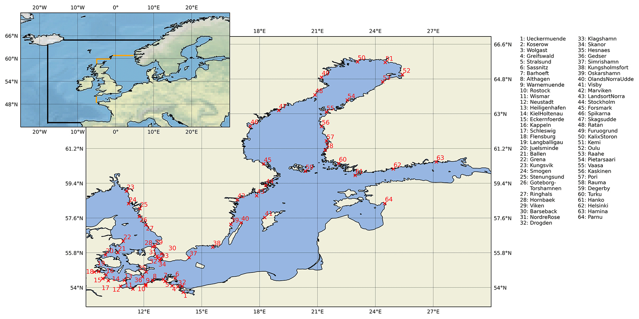
Figure 1Model domain and locations of the stations (red crosses and numbers) used for validation. The black line indicates the boundary of the coarse Northwest Atlantic Ocean domain. The orange lines mark the boundaries of the 1 NM setup of the North Sea and Baltic Sea.
2.1 Numerical Simulations
We use the General Estuarine Transport Model (GETM (version 2.5), Burchard and Bolding, 2002), a structured coastal ocean model (Klingbeil et al., 2018), to simulate the surface elevation in the Baltic Sea. The model has been widely used for many Baltic Sea applications, including storm surges: Gräwe and Burchard (2012). Here, we use the GETM to solve the vertically integrated shallow water equations, considering only barotropic effects and ignoring baroclinic processes (except for one simulation where we include static baroclinic circulation). We employ the superbee advection scheme (Pietrzak, 1998). The wind stress is calculated from the 10 m wind fields with
with ρair=1.25 kg m−3 and the 10 m wind speed vector u10. The drag coefficient CD is computed by the formulation of Kara et al. (2000). In our barotropic simulations we do not consider temperature differences between the ocean and atmosphere. Therefore, the drag coefficient reads as
where the wind speed is limited: . The numerical setup of the Baltic Sea has a resolution of 1 NM, which is nested into a coarse (5 NM) model of the Northwest Atlantic with a bottom roughness of z0=0.005 m (see Fig. 1), similar to the setups of for example Gräwe et al. (2015). The Northwest Atlantic model is forced with ERA5 (Hersbach et al., 2020) with unchanged wind speeds. Along its boundary, air pressure-induced water-level changes are imposed using the atmospheric pressure from ERA5 to include large pressure systems from the Atlantic in the model chain (inverted barometric effect). This simulation prescribes boundary conditions for the 1 NM North Sea and Baltic Sea domain (all simulations). This may introduce some inconsistencies in the sea level when using other atmospheric forcings for the North Sea and Baltic Sea nesting stage. However, we assume these errors to have little effect on Baltic Sea ESLs as the Danish Straits act as a low-pass filter. Thus, ESLs are generated inside the Baltic Sea as a superposition of storm surges, filling states, and local seiches, which are all included in the model setup. Note that the boundary conditions for this nesting do not include tides to avoid introducing tide–surge interactions (Arns et al., 2020). Tides are negligible for the Baltic Sea, as explicitly shown by Gräwe and Burchard (2012). However, standing wave–surge (seiche–surge) interactions (Arns et al., 2020) are included. Furthermore, the mean sea level is kept constant in order to study only the atmospheric-induced extreme sea levels themselves (ESL distributions treat the mean sea level as a linear term (Coles et al., 2001)). The North Sea and Baltic Sea domain is set up with a bottom roughness of z0=0.001 m, a value that is also used by coastal ocean models other than the GETM for the Baltic Sea (e.g. Kärnä et al., 2021).
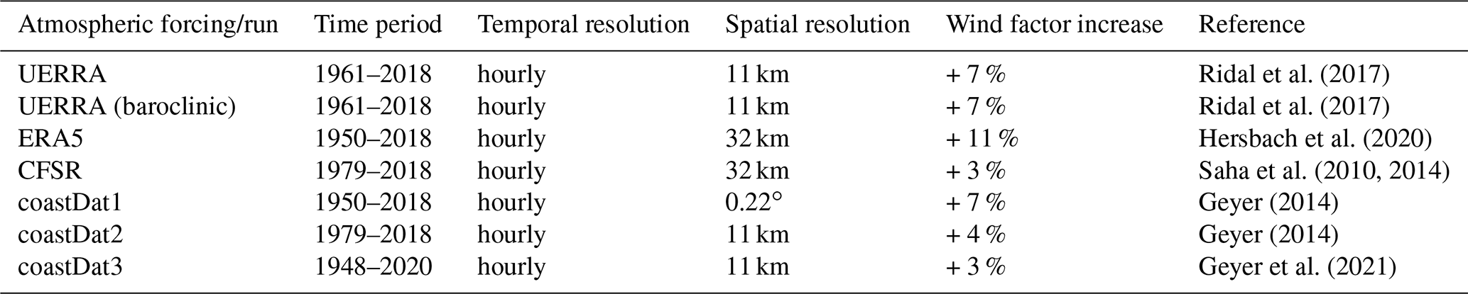
High-resolution atmospheric forcing in both time and space is required to model extreme sea levels. For the Baltic Sea, we consider the regional atmospheric reanalyses listed in Table 1, which provide the high-resolution fields needed for wind speeds (10 m height) and sea-level pressure. For this study, we investigate the period from 1979 to 2018, the overlap between all atmospheric datasets, focusing on the variability between these ensemble members. We included one run (“Uncertainties in Ensembles of Regional ReAnalyses (UERRA) baroclinic”) where we included monthly mean static density fields and static ice cover (taken from Gräwe et al., 2019). For each atmospheric forcing, we ran one simulation with default wind speeds (directly taking the values provided by the atmospheric dataset) and one with increased wind speeds (see Table 1), for a total of 13 ensemble members. Before all analyses, we subtracted the linear trends from each time series to explicitly consider only ESLs relative to the respective mean sea level. This excludes changes in the mean sea level due to persistent changes in wind speed, wind direction, sea-level pressure changes, and external loading (Gräwe et al., 2019).
Ridal et al. (2017)Ridal et al. (2017)Hersbach et al. (2020)Saha et al. (2010, 2014)Geyer (2014)Geyer (2014)Geyer et al. (2021)Table 1Overview of the different atmospheric datasets used in this study. Each atmospheric forcing is included one time with default wind speeds and one time with increased wind speeds except the Uncertainties in Ensembles of Regional ReAnalyses (UERRA) (baroclinic) run, which is only computed with increased wind speeds.
2.2 Observational Gauge Data
We use several gauges to validate the model results along the Baltic Sea coastline. The data are obtained from the European Marine Observation and Data Network (EMODnet, https://emodnet.ec.europa.eu, last access: 5 June 2021) and the Global Extreme Sea Level Analysis (GESLA, Woodworth et al., 2016; Haigh et al., 2022). From both sources we have obtained quality controlled sea-level data of hourly frequency. The sea-level data are accurate to within 1 cm. The station record lengths and data gaps are summarised in Fig. 2 (a table of the gauges is provided in Table S1 in the Supplement). Their locations are shown in Fig. 1 and also listed in Table S1 in the Supplement. Note that we only included stations with time series starting in 2004 and earlier, and that we use the data from 1979 onwards to match the simulation periods. For each gauge, the mean sea-level rise is subtracted (linear fit over the entire time series) before analysis and comparison with model results. This also excludes sea-level changes due to GIA from the tide gauges. For the direct comparison of ESL events with observations (Sect. 3.1), we use the German Federal Maritime and Hydrographic Agency's definition of a storm surge in the Baltic Sea. It defines a storm surge as a sea level of more than 1 m a.m.s.l.
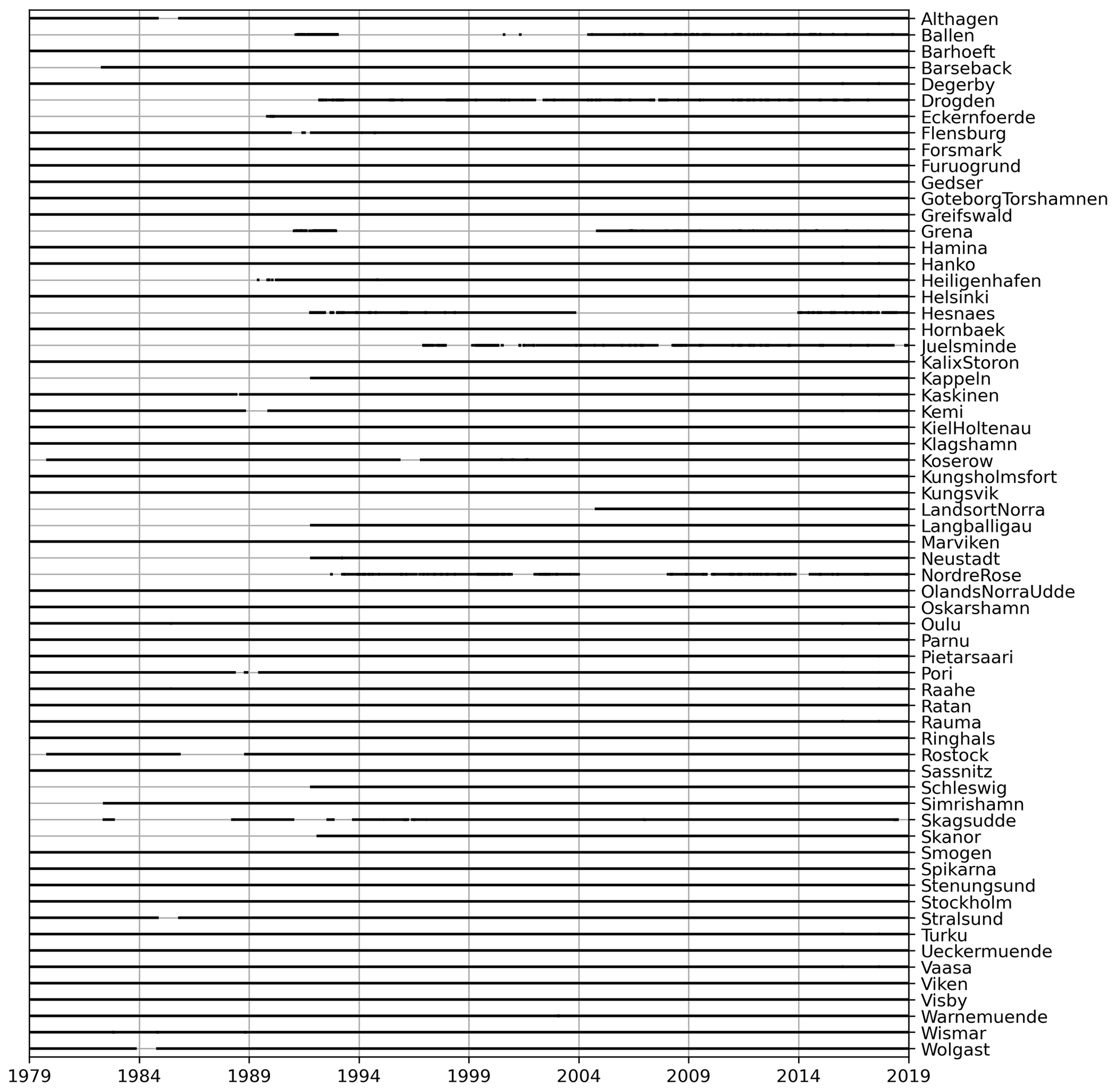
Figure 2Overview of the record lengths and data gaps of the gauge stations. A table with exact locations and more details of the exact time spans and gaps can be found in the Supplement in Table S1.
2.3 Extreme Value Statistics
We emphasise that we assume that the statistical properties of the extreme value distributions are constant in time within the considered time frame. Therefore, we do not consider temporal changes in the extreme value distributions. This assumption may not be valid (Kudryavtseva et al., 2018, 2021). However, this study focuses on the variability within the ensemble and not on the comparison between static and temporally varying extreme value distributions.
2.3.1 Generalised Extreme Value Distribution
To describe the distribution of storm surge heights and return periods, we use the generalised extreme value (GEV) distribution (Coles et al., 2001) using the time series of annual storm season (July to June) block maxima (Männikus et al., 2020). The GEV (cumulative distribution function) is defined by
where z is the sea level, μ is the location parameter, σ is the scale parameter, and ξ is the shape parameter. The shape parameter ξ governs the tail of the distribution and depending on its value the distribution reduces to
-
Gumbel distribution for ξ→0:
-
Fréchet distribution for ξ>0:
-
Weibull distribution for ξ<0:
For each gauge used in this study, the GEV is fitted to the annual storm season maxima. We use the Python code from Reinert et al. (2021) for the fitting, which uses the maximum likelihood estimation method.
2.3.2 Generalised Pareto Distribution
Another function to describe the statistical distribution of extreme values is the Generalised Pareto Distribution (GPD) (cumulative distribution function),
where is the scale parameter, , and u is the threshold (Coles et al., 2001). This method uses a peak-over-threshold to sample the time series (minus the mean sea-level rise). In this study, we use the 99.7 % percentile of the sea-level distribution as the threshold suggested by Arns et al. (2013) and only consider events separated by more than 48 h. We use the maximum likelihood estimation method and a Python script for the fitting.
3.1 Comparison of sea levels
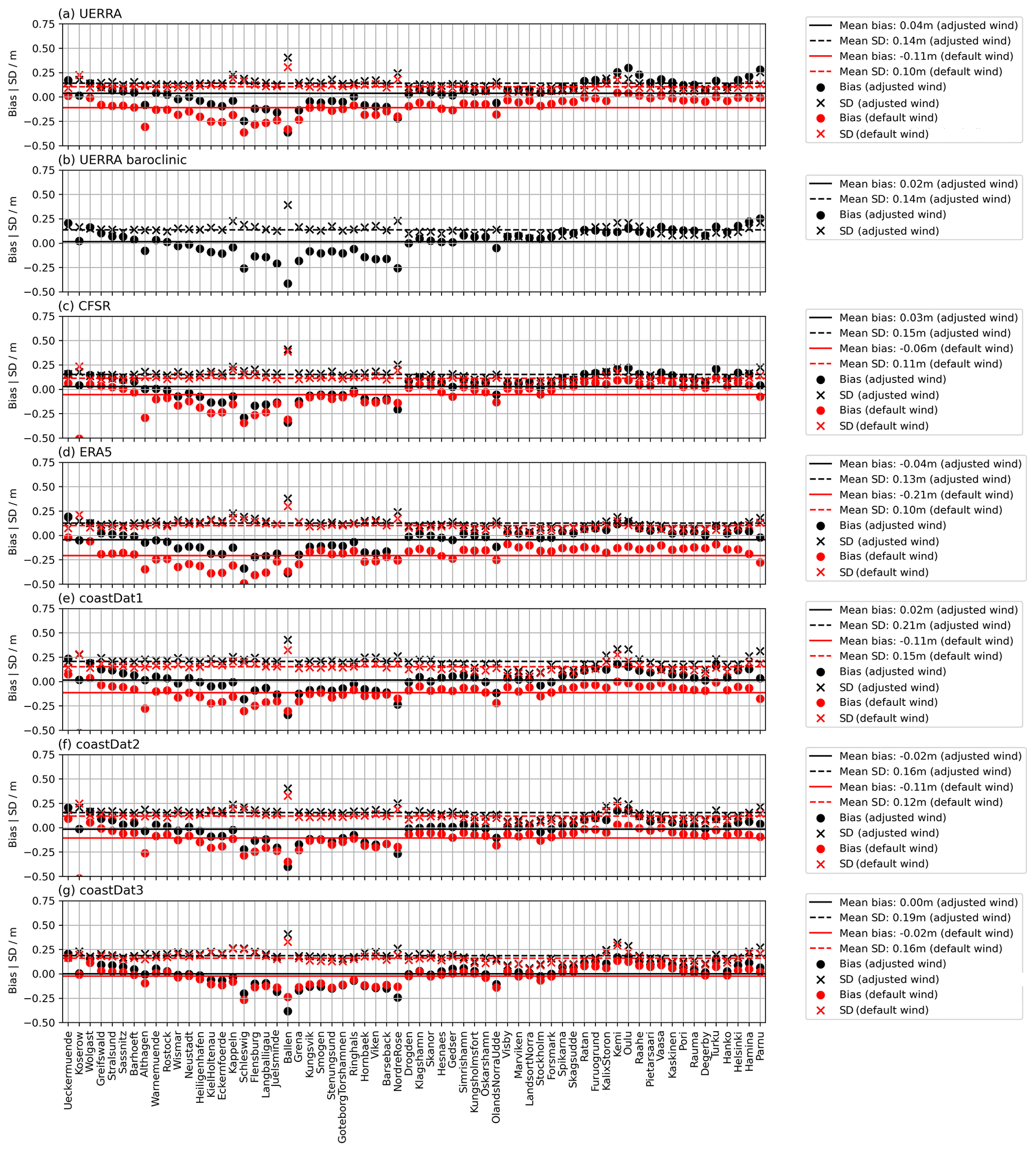
As we are interested in the ESLs, we compare the observed ESLs for each station with the modelled ESLs (Fig. 3), where the stations are sorted in a clockwise direction along the Baltic Sea coast, starting from the Western Baltic Sea (Fig. 1). The time-series comparison for each tide gauge station shows a good agreement with low Root Mean Square Errors (RMSE≤0.1 m) and high Pearson correlation coefficients R≈0.9 (see Fig. S1). Furthermore, we only consider events that are separated by more than 48 h. We search for events that fulfil these criteria in the observed tide gauges and compare them with the modelled sea level for each station. This comparison shows that the default wind-speed simulations have a clear negative mean bias, red dots and values in Fig. 3. On average, the simulations underestimate the maximum water levels. The bias is different for each atmospheric forcing. To improve this comparison of ESLs in the model, we increased the wind speeds by a constant factor for each atmospheric dataset (see Table 1). With this increase, the mean bias of the model results reduces significantly (see black dots and values in Fig. 3). However, it should be kept in mind that, owing to the homogeneous wind-speed increase, some areas, i.e. stations, in the model domain show a larger bias than before, e.g. the central and Northern Baltic Sea. However, the wind speed increase is necessary to capture the correct ESLs in the Western Baltic Sea. Therefore, in the following analysis of the ESLs, we consider both the default simulations (larger mean bias) and the simulations with adjusted wind speeds (smaller mean bias) as an ensemble of 13 members. Note that the ESLs for stations in shallow coastal lagoons such as “Althagen” and “Schleswig” are overestimated because the model does not resolve the local topography and inlets.
3.2 Return levels and variability within the ensemble
3.2.1 Return levels obtained from the GEV method
As the period considered is only 40 years, we compare the 30-year return periods, which should be well estimated by the underlying 40 years of data (see also Gräwe and Burchard (2012)). The comparison of modelled and observed 30-year return levels for the stations (Fig. 4) shows a large variability between the atmospheric reanalyses. A more detailed view of all return level fits and the different simulations' confidence intervals is shown in Fig. S2 for the station “Warnemuende” in the Supplement. We have again sorted the stations clockwise around the Baltic Sea coast, starting in the Western Baltic Sea. This depiction shows that the default wind-speed simulations have a clear negative bias in the Western Baltic Sea but show good agreement in the central and Northern Baltic Sea regions. On the other hand, the adjusted wind-speed simulations show good agreement in the Western Baltic Sea and an overestimation in the central and Northern regions. This pattern is similar to the general comparison of ESLs in Sect. 3.1. This shows that the biases from the previous section are directly reflected in the return-level estimates. Each atmospheric forcing has its strengths and weaknesses regarding how well storm systems are represented in terms of intensity and tracks in different regions. Therefore, the spatially homogeneous adjustment of wind speeds improves the representation in some areas but causes it to deteriorate in others. However, these problems seem to cancel out for the ensemble (Fig. 4h). For most of the stations, the ensemble mean return level is close to the mean return level based on the observations and well within the respective 95 % confidence interval.
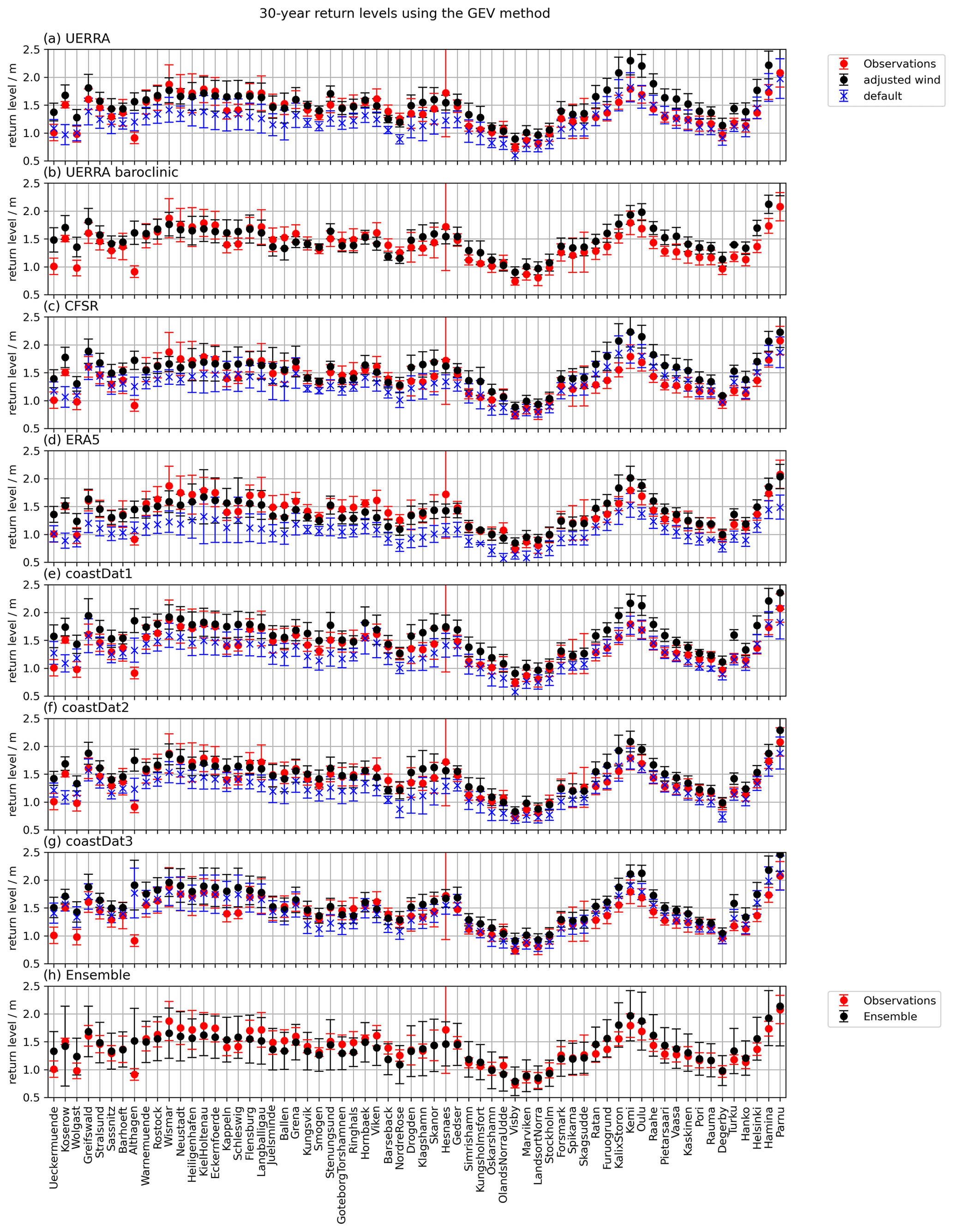
Figure 4Summary of the 30-year return levels using the GEV method for each gauge station and each ensemble member: (a)–(g) return levels and 95 % confidence intervals for each atmospheric forcing and each simulation. (h) ensemble mean and ensemble 95 % confidence interval. The large 95 % confidence interval of the station “Hesnaes” is explained by a large uncertainty of the fitted shape parameter ξ.
Using the model to fill the area between the observed gauges, we show the ensemble mean 30-year GEV return level for every fourth data point (every second point in latitude and longitude) in the Baltic Sea (see Fig. 5a). As westerlies are the dominant winds in the Baltic Sea region, the eastern coasts show higher return levels as expected and well documented (e.g. Wolski et al., 2014). In the South-Western Baltic Sea, west-facing coasts have higher return levels than those facing north or south but lower expected return levels than the Northern and Eastern Baltic Sea. Although the ensemble mean shows good agreement with the estimated return levels based on the observations, the spread, i.e. the 95 % confidence interval, shows large values up to 50 cm and more (Fig. 5b).
Comparing the different ensemble members with the ensemble mean (Fig. 6) we see more clearly how each member has its regions where it is close to the ensemble mean and regions where it deviates strongly. This depiction shows that the general pattern of the high and low return levels is similar in each simulation, but the estimated return levels vary considerably, as already seen previously. Without again describing the spatial pattern of each ensemble member, we want to emphasise the discrepancies between the individual simulations. Generally, the adjusted wind-speed simulations are at the high end of the distribution, whereas the default wind speed simulations are at the low end. The simulation with the lowest return levels is ERA5. The simulation with the highest return levels is the UERRA simulation, which includes the increased wind speeds and incorporates static density effects. Already when comparing the default simulations, the differences between the 30-year return levels of these six simulations can be as high as 60 cm, even though they are all reanalyses.
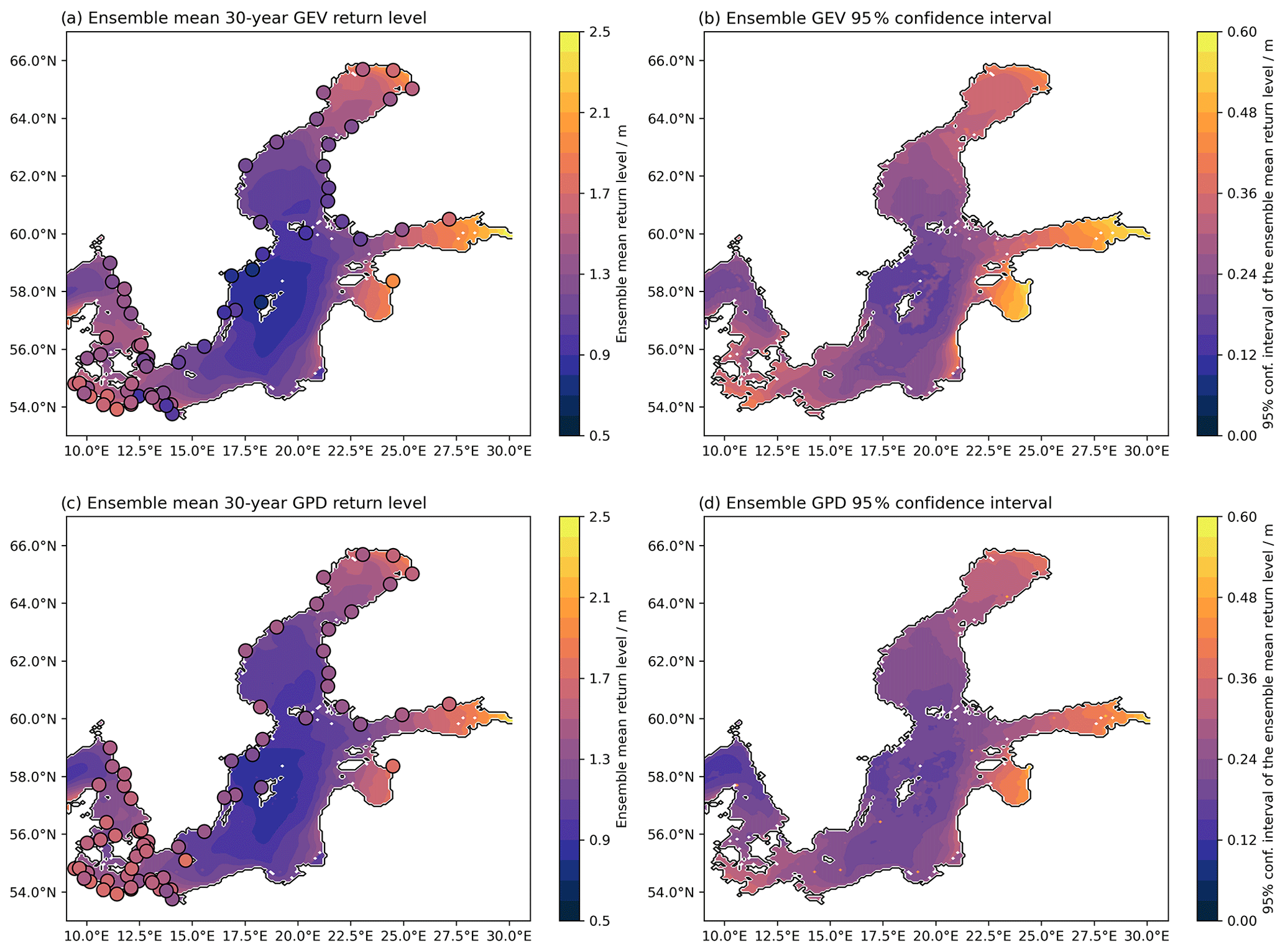
Figure 5Maps of the return levels and the 95 % confidence intervals. (a) Ensemble mean of the 30-year GEV return levels. (b) The 95 % confidence interval of the GEV return levels. (c) Ensemble mean of the 30-year GPD return levels. (d) The 95 % confidence interval of the GPD return levels. In (a) and (c), the coloured dots indicate the 30-year GEV and GPD return levels of the observations.
3.2.2 Return levels obtained from the GPD method
Similar to the return levels estimated by the GEV method, we estimated the return levels based on the GPD method for the same period. In the Supplement, we provide plots comparing the estimated return levels of the simulations with the return levels based on the observations: for the station “Warnemuende” in Fig. S3 and for the 30-year return levels in Fig. S4. In short, comparing the 30-year return levels for each station, the patterns are similar to the GEV results, except for the generally lower estimates for the 30-year return levels. Again, the adjusted wind-speed simulations are in better agreement with the observations for the Western Baltic Sea than for the Northern and Eastern Baltic Sea, where the default wind speed simulations are in better agreement with the observations. Overall, based on the observations, the ensemble mean 30-year return levels lie within the 95 % confidence intervals of the 30-year return level estimates.
The general pattern of high and low GPD 30-year return levels (Fig. 5c) is very similar to the pattern of high and low GEV 30-year return levels in Fig. 5a. Also, the spatial GPD 95 % confidence interval pattern and the values are similar to the GEV 95 % confidence interval (Fig. 5b and d). This suggests that the uncertainty within the ensemble is independent of the method used to estimate the return levels. This claim is supported by the deviations of the 30-year GPD return levels from the ensemble mean (Fig. S5 in the Supplement). Each ensemble member shows similar deviations (both in pattern and values) to the GEV return levels in Fig. 6.
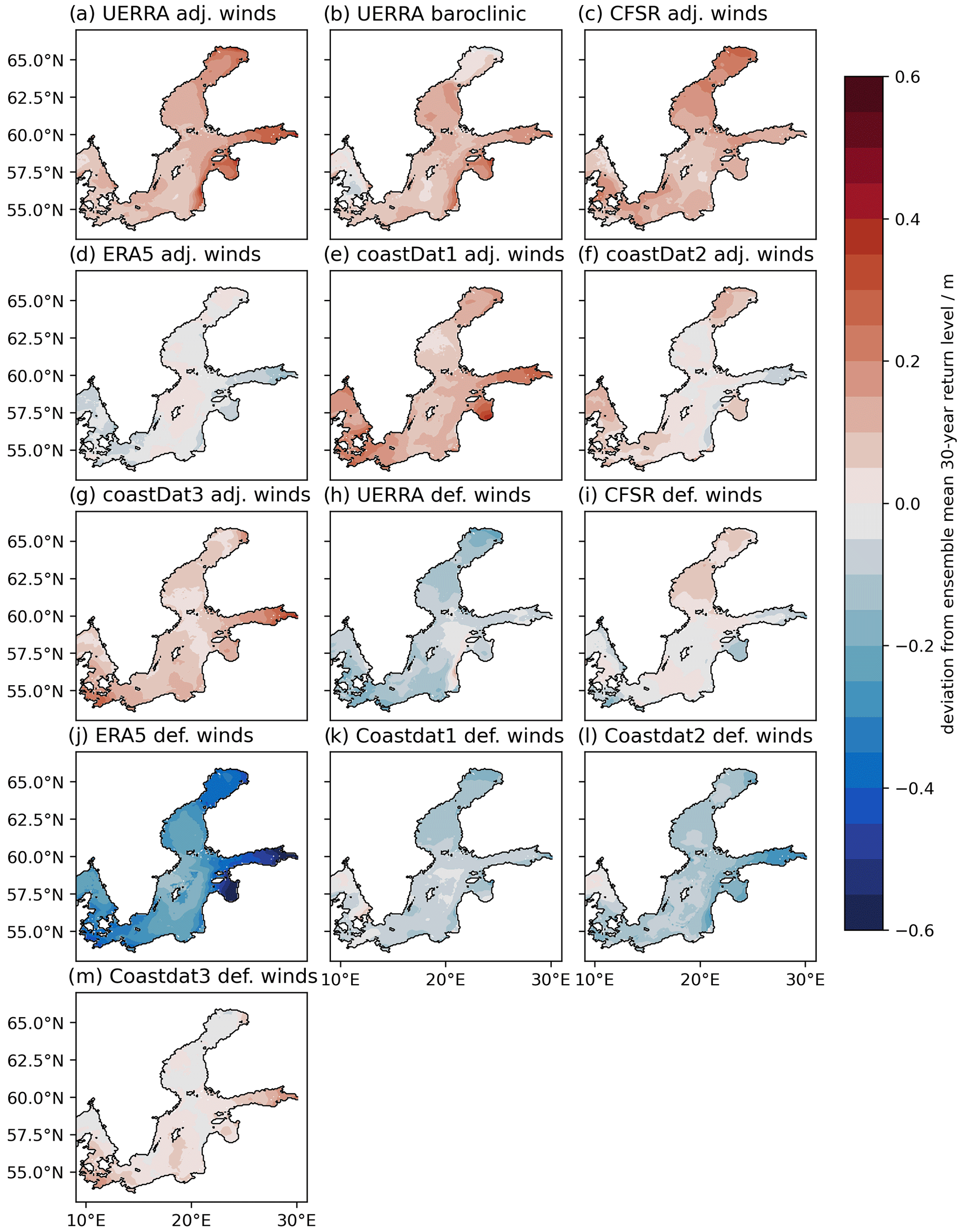
Figure 6Spatial distribution of the 30-year GEV return level deviation from the ensemble mean (see Fig. 5a) for each ensemble member.
3.3 Trends
We have seen in the previous sections that the modelled ESLs differ from observations to a different extent for each atmospheric forcing. Therefore, the estimated 30-year return levels differ significantly within the ensemble, leading to significant uncertainty. Previous studies have shown some trends in storm surge occurrence and heights. Therefore, we look at linear annual storm season maxima trends within the ensemble period, 1979–2018. For the ensemble mean (Fig. 7) we find a negative mean trend in the Baltic Sea except for the eastern Kattegat and the waters north of Poland. The ensemble mean shows the largest negative trends in the Northern Baltic Sea and the Gulf of Finland. However, the uncertainty within the ensemble is large, up to 1.5 mm yr−1 (Fig. 7b). Comparing the trends with the observed trends (coloured dots in Fig. 7a), we see a general agreement in the trends and in the spatial distribution. However, some gauge stations show deviations in the sign of the trend, e.g. stations in the Western Baltic Sea. This indicates that details in the trends are not captured by either the ocean model resolution (1 NM) or the atmospheric reanalysis data.
Comparing the trend of each member (Fig. 8), we see an agreement in the spatial pattern of trends, as represented by the ensemble mean. However, the size and shape of the areas of positive and negative trends differ, e.g. the extent of the area in the Western Baltic Sea that shows a positive trend varies for each ensemble atmospheric forcing. Furthermore, the actual values of the trends differ greatly within the different simulations, not only between the adjusted and default wind speeds but even within the sub-sample of default simulations.
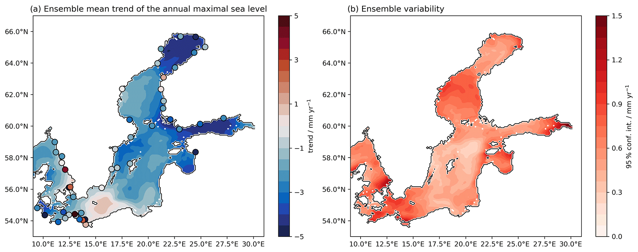
Figure 7The ensemble mean trend in (a) and the 95 % confidence interval of the mean trend of the annual storm season maxima in (b) for the time period from 1979 to 2018. The coloured dots show the trends of the tide gauges covering the same 40 years. Note that the mean sea-level trends have been subtracted beforehand.
From the results of our study, we find that the choice of atmospheric reanalysis has a significant impact on how well the ocean model simulates past sea-level extremes. Not only are the estimated return levels significantly different depending on the choice of the atmospheric reanalysis, but the modelled trends in sea level maxima are also affected. One of the reasons is that each simulation forced by a different reanalysis product underestimates or overestimates different ESL events as each real storm system is represented slightly differently. Furthermore, each reanalysis has different biases, both spatially and in wind speed distribution and direction. Therefore, the variability within the generated ensemble can be quite large, both for the return levels and for trends. Nevertheless, the ensemble mean can reproduce observed return levels and observed trends.
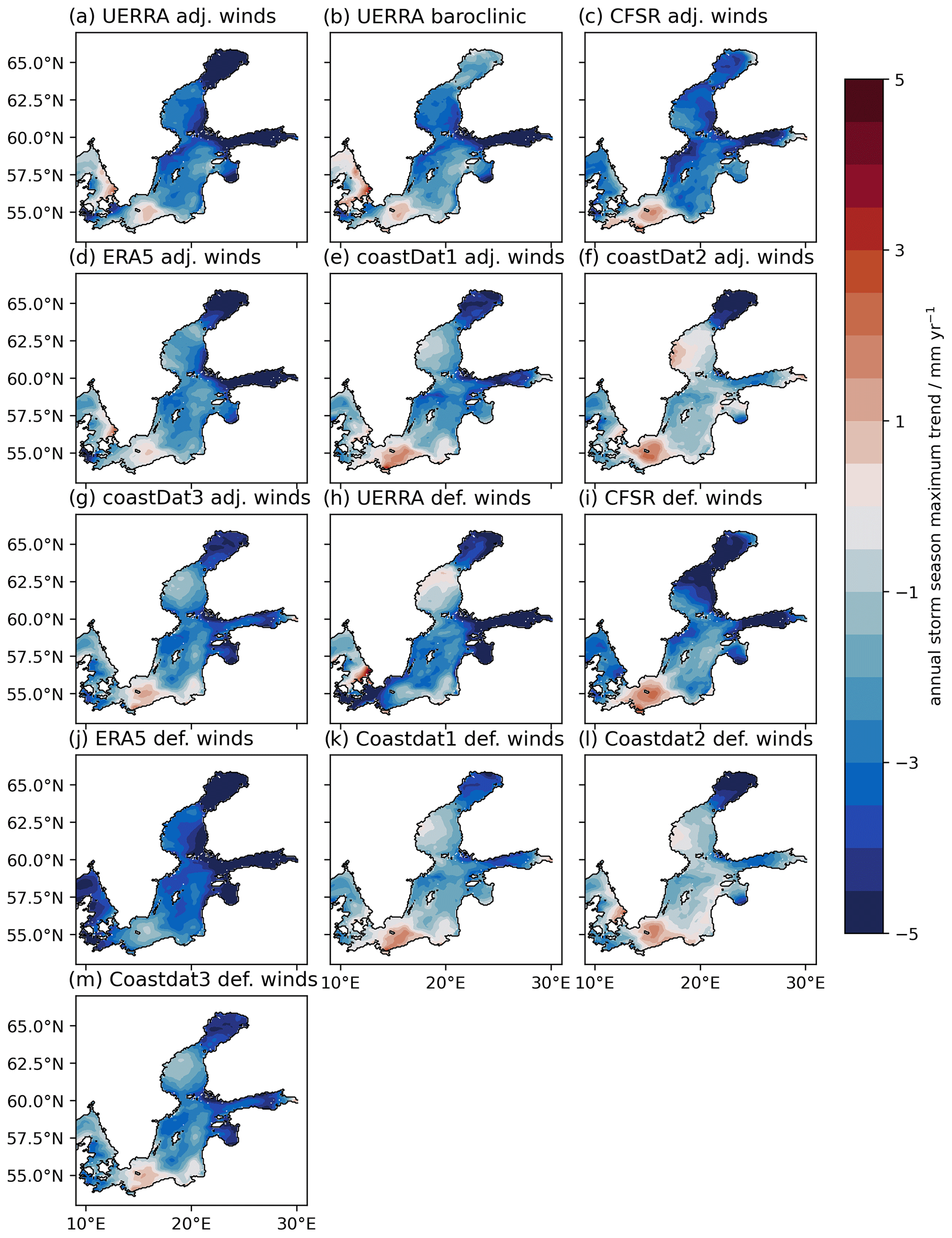
Figure 8Trend in each ensemble member's annual storm season maxima. Note that the mean sea-level trends have been subtracted beforehand.
The variability within the ensemble for the 30-year return levels can be as high as 60 cm in the Gulf of Finland or the eastern part of the Baltic Proper. Along the western coasts of the Baltic Sea, the 95 % confidence values are around 30–40 cm. The 99th percentiles for each default 10 m wind speed (u10) dataset from Table 1 (Fig. 9) show the variability between the different datasets. ERA5 has the lowest ESLs and has the lowest 99th percentile wind speeds over the Baltic Sea. The Climate Forecast System Reanalysis (CFSR) shows the highest 99th percentile wind speeds over the Baltic Sea of the ensemble, which translates into the smallest adjustment for wind speeds of 3 % (Table 1). The 95 % confidence intervals due to the variability within the ensemble are ∼2.5 m s−1 between the default atmospheric datasets over the entire Baltic Sea. This can result in a difference in the maximal sea levels of approximately
where L is a distance scale (fetch length) (𝒪(L)=100 km), the drag coefficient CD, which is approximated at 0.001 for simplicity, the density of air ρair≈1.25 kg m−3, the density of seawater ρ0≈1000.0 kg m−3, the water depth H, and g the gravitational constant. The sea-level difference depends strongly on the water depth and the distance L. For u10=18.0 m s−1, L=300 km, and H=50 m, the resulting elevation change would be ∼43 cm. The resulting sea-level change would be even higher for shallower waters or greater distances. This approximation of the effect of the atmospheric variability is in the order of magnitude of the sea level confidence interval of the ensemble. This highlights the importance of correctly representing high-percentile wind speeds, i.e. storms, in the atmospheric reanalysis, to capture the ESLs in the simulations. The variability within the ensemble of our study is in agreement with other studies in this regard: Dieterich et al. (2019) discuss the historical period (1961–2005) of a regional climate model for the North Sea and the Baltic Sea to study the variability within an ensemble of six members (six different global model boundary conditions for their regional general circulation model). They find uncertainties between 20 and 40 cm added by the choice of the global circulation model boundary conditions as the largest uncertainty for the 100-year return levels. Eelsalu et al. (2014) show for their small three-member ensemble for the Estonian coast that uncertainties for 15-year return levels are within the range of about 20 cm. However, for longer return periods, their spread grows significantly to 60 cm or more. In general, the errors grow with longer return periods, as does the variability of our ensemble. To reduce the uncertainty, we believe a large regional ensemble is needed.
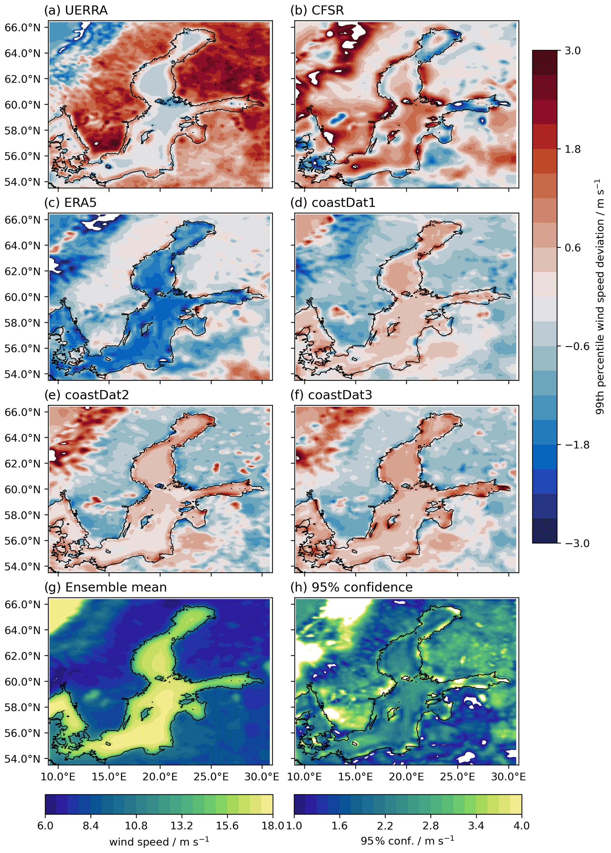
Figure 9Deviations of the 99th percentiles of the 10 m wind speeds from their mean for the meteorological forcings used to generate the ensemble. The mean in (g) and the standard deviation in (h) are computed by interpolating the individual percentiles of each forcing onto the grid of the UERRA dataset.
The variability of the return levels within the ensemble is independent of the choice of chosen extreme value distribution. Our results show similar confidence intervals within the ensemble for both the GEV and GPD methods: both show similar spatial patterns and similar values. However, their absolute values for the return levels differ, especially for the short and very long return periods. Based on the annual maxima of the storm season, the GEV method yields higher 30-year return levels than those obtained from the GPD method. We do not want to discuss the pros and cons of the methods. We refer to Arns et al. (2013) for a detailed discussion of this. However, the difference in the return levels of the two methods for the 30-year return levels shown in this study is smaller or within the range of variability within the ensemble. This indicates that future efforts should be made to minimise the uncertainty. ESLs are the superposition of many sea-level processes: preconditioning, storm surges, and standing waves (seiches). For example, as preconditioning can increase the mean sea level in the Baltic Sea on weekly time scales, the total sea level during a storm surge can be increased. These two (or more) compounding mechanisms follow different statistical distributions (e.g. Suursaar and Sooäär, 2007), which can be extracted by separating the time series into different temporal components (Soomere et al., 2015). Our analysis neglects this point as the GEV and GPD methods assume a single statistical distribution that still led to good fits. Furthermore, the mentioned mechanisms are interacting non-linearly (Arns et al., 2020). Disentangling these two (or more) compounding processes (Soomere and Pindsoo, 2016; Pindsoo and Soomere, 2020) of this ensemble remains a matter for a future study.
We have shown with the generated ensemble that the trend of the annual storm season maxima is different for each ensemble member, but still shows some agreement in the general spatial pattern. As each storm is captured differently in each atmospheric dataset, this influences the trends of the ESLs. Figure 10 shows the linear trends of the annual 99th percentile wind speeds for each dataset and the ensemble mean (interpolated to the UERRA grid). The datasets agree on negative trends for the southern, western, and central Baltic Sea for the hindcast period. We found a positive trend for most datasets for the northern and eastern parts. CoastDat2 deviates from this general pattern with very small trends in the Western Baltic Sea and negative trends in the north. As the CFSR member is forced with both CFSR and CFSv2 no consistent model is used and the trends shown are expected to be mostly due to the change in the model configuration. An estimate of how the wind trends can be translated into sea-level trends can be made using the derivative of Eq. (7):
where the value ∂tX denotes the slope of the trend line. For u10=18.0 m s−1, L=300 km, and H=50 m, and m s−1 yr−1 the resulting change in elevation would be ∼0.7 mm yr−1. However, the ensemble trends of the sea level maxima are higher, indicating that directional changes and preconditioning must play a critical role. However, this is beyond the scope of this study. Furthermore, if we compare the trends of the ensemble mean with the results of Soomere and Pindsoo (2016) and Pindsoo and Soomere (2020), we find an apparent discrepancy. Whereas Soomere and Pindsoo (2016) and Pindsoo and Soomere (2020) find a clear positive trend of up to 10 mm yr−1, the ensemble of this study shows a negative trend. They further show that preconditioning is responsible for up to 4–5 mm yr−1 of the total trend, showing that preconditioning does indeed play a crucial role. It should also be noted that these trends are sensitive to the considered period as the natural variability of the Baltic Sea region includes oscillations in the order of decades owing to the North Atlantic Oscillation (NAO) and the Atlantic Multidecadal Oscillation (AMO) (also named Atlantic Multidecadal Variability, AMV) (Meier et al., 2022b, and references therein). The considered time period of Soomere and Pindsoo (2016) and Pindsoo and Soomere (2020) is from 1961 to 2005 with a 6-hourly model output. We compared the trends for the tide-gauge station, which go back to 1961 for both time periods, 1979–2018 and 1961–2005 (Table S2). The results show that both time periods lead to different trends, even changing the sign of the trend. Many of these stations show a positive trend for 1961–2005 and negative trends for 1979–2018. For example, stations in the Western Baltic Sea show a positive trend up to 4 mm yr−1, which is in agreement with the previous studies. However, this is not the case for “Parnu”, which still shows a negative trend. Therefore, the discrepancy between this study and previous studies can be only partly attributed to the different time periods. This hints that the variability of ESLs to the NAO and AMO/AMV should be revisited. Furthermore, the 6-hourly output of Soomere and Pindsoo (2016) and Pindsoo and Soomere (2020) could introduce some aliasing as peak water levels may not be captured (compare with, for example, Kiesel et al. (2023) for mean time series of ESLs in the Western Baltic Sea).
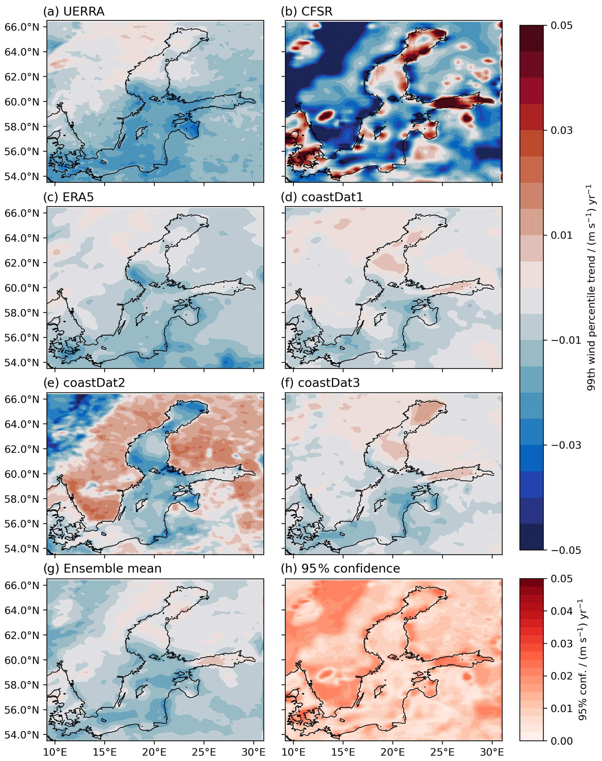
Figure 10Trend of the annual 99th percentiles of 10 m wind speeds for the meteorological forcings used to generate the ensemble.
Our ensemble has a record length of 40 years. The 100-year or 200-year return levels are often used as protection targets for coastal protection planning. Therefore, an extrapolation of the data leads to significant uncertainty ranges (see, for example, Figs. S2 and S3 in the Supplement, where the confidence intervals grow significantly when extrapolating, especially for the GEV method). To reduce the uncertainties, longer time series would be necessary to estimate the long return periods reliably. For the Baltic Sea, very long (>100 years) time series exist and have been used to study the large return levels (e.g. Suursaar and Sooäär, 2007). However, our results show that climate change makes reliable estimates of the highest return levels for the current and future climate states based on small ensembles or single simulations that are complicated and uncertain (see also Muis et al. (2022)). It is expected that the underlying statistical distribution will change with climate change. Therefore, non-stationary extreme value statistics have been used in other studies, e.g. Kudryavtseva et al. (2021), and temporal trends in ESLs have been studied, e.g. with quantile regression (Barbosa, 2008). Disentangling these changes in statistical extreme value distributions is only possible with numerical models. However, much larger ensembles are needed to separate ensemble variability from changes due to climate change. Currently, the ensemble variability for climate scenarios for the European coasts is in the order of magnitude of the expected differences between low and high Representative Concentration Pathway (RCP) scenarios (e.g. Vousdoukas et al., 2017). In addition, the large natural variability in the Baltic Sea region makes this disentanglement even more complicated.
To reduce model bias (Sect. 3.1), we increased the wind speeds by a constant factor, which reduced the mean bias of ESLs. However, the results suggest that the wind factor should be varied spatially to account for regional biases in ESLs in the simulations. The main negative model bias in our study, but also in previous studies, is found in the ESLs of the Western Baltic Sea. In early model studies the bias was because of coarse resolution, which allowed water to exit through the Danish Straits during ESL events (e.g. Meier et al., 2004). Furthermore, local convergence effects need high model resolution to be correctly reproduced. But negative biases in ESLs are also found in high-resolution hydrodynamic models: 1 km resolution in Gräwe and Burchard (2012), 200 m resolution in Kiesel et al. (2023). Therefore, biases can be attributed to wind-speed biases (e.g. Gräwe and Burchard, 2012). In the present study, we found the ESL biases to be caused by biases in the atmospheric datasets or how the ocean model translates the forcing into sea level changes. Applying better corrections is not a trivial undertaking and would certainly further disturb the physical consistency. Adjusting wind speeds may help with the biases in the ESLs, but it also has implications for general hydrodynamics, which is not the focus of this study. Because we use vertically integrated Reynolds averaged Navier–Stokes equations, we do not consider changes in the surface mixed layer depths, or upwelling and downwelling. Nevertheless, these would be strongly modified by the adjusted wind speeds and may lead to over- or underestimation of these. This would have consequences for the general dynamics, e.g. stratification or the total salt import by Major Baltic inflows. One possible way of tackling this problem could be adjoint and inverse models (Errico, 1997), which can be used to calibrate coastal ocean input fields such as bottom friction (Kärnä et al., 2023) or in this case wind speed factors. However, this does not solve the underlying issue, which we believe is found in the resolution of the atmospheric models over the Western Baltic Sea. Compared with the size of the Western Baltic Sea, the number of grid cells in the atmosphere is probably not high enough to resolve the winds properly.
Many formulations, i.e. polynomial fits, of the drag coefficient exist that translate wind speeds into wind stresses (e.g. Kara et al., 2000; Large and Yeager, 2009). Here we have used the formulation of Kara et al. (2000). Using a different formulation, e.g. one that yields a larger drag coefficient for high wind speeds, could have improved the representation of ESLs and potentially decreased the wind factors we applied. As there are many formulations, each formulation would lead to different ESLs, thus introducing a source of variability. The different formulations depend on the geographic locations of the underlying data, which are fitted, e.g. offshore versus onshore (Smith et al., 1992). The formulation we have used (Kara et al., 2000) is based on observations made in the Arabian Sea. One could argue that this formulation may not be suitable for the Baltic Sea. However, we expect for this study that the variability of the atmospheric datasets, Figs. 9 and 10, to be much larger than the differences in ESLs owing to the drag coefficient formulations. Still, the exploration of the effect of different drag coefficient formulations on ESLs in the Baltic Sea should be carried out in a future study. A calibrated drag coefficient formulation using an adjoint model could be a possible solution (Peng et al., 2013). However, depending on the wind input fields, different best fits have to be expected.
We have increased the ensemble spread by including the default and adjusted wind-speed simulations. We could have either used only the default wind-speed simulations and accepted the negative biases in the Western Baltic Sea, thus reducing the ensemble spread, or we could have included them to improve the ensemble mean for that region, with the drawback of larger uncertainties. Ultimately, uncertainties are shifted from one problem to another and would not be minimised.
We show that modelling extreme sea levels is difficult and relies heavily on correctly representing storms in the atmospheric forcing data. We derive and provide a 13-member hindcast ensemble focusing on extreme sea levels, covering the period from 1979 to 2018. We constructed the ensemble using present state-of-the-art reanalysis datasets for the Baltic Sea region. We have explicitly not considered long-term changes in mean sea level. The ensemble mean can reproduce similar extreme value distributions to tide gauges around the Baltic Sea, both for the Generalised Extreme Value (GEV) distribution and the Generalised Pareto Distribution (GPD). However, spatially heterogeneous biases can be expected depending on the choice of atmospheric forcing. We find a large variability within the ensemble: up to 60 cm (95 % confidence interval) within the ensemble for the 30-year return levels and trend variability up to 1.5 mm yr−1 for the annual maximum sea level. This variability is entirely due to the different atmospheric representations of storms and how these translate into the sea-level computation in the ocean model. One approach to trying to minimise this uncertainty can be the use of much larger ensembles. Hence, we invite other scientists to incorporate our numerical simulations and results into future ensembles to increase the number of ensemble members. Initiatives such as the Baltic Sea Model Intercomparison Project (BMIP, Gröger et al. (2022), https://www.baltic.earth/working_groups/model_intercomparison/index.php.en, last access: 13 September 2023) should therefore be expanded in the future to build a large regional ensemble with multiple forcing combinations.
As the trends of annual maximum sea levels are sensitive to the time period considered and the trends of this study differ from previously published studies (e.g. Soomere and Pindsoo, 2016; Pindsoo and Soomere, 2020), we believe that the dependence of ESLs on the NAO and AMO/AMV should be reconsidered. Furthermore, the contributions of preconditioning, seiches, and surges to ESLs in the context of climate modes need to be disentangled.
The results, a frozen GETM version, and the analysis code can be found here: https://doi.org/10.5281/zenodo.8340649 (Lorenz and Gräwe, 2023a). The model output can be accessed here: https://iowmeta.io-warnemuende.de/geonetwork/srv/eng/catalog.search#/metadata/IO W-IOWMETA-BalticSeaExtremeSeaLevelHindcastEnsemble-197 9-2018 (Lorenz and Gräwe, 2023b). The atmospheric forcings can be accessed from the following links: UERRA https://doi.org/10.24381/cds.44ec8078 (Copernicus Climate Change Service, 2019), ERA5 https://doi.org/10.24381/cds.adbb2d47 (Hersbach et al., 2023), CFSR https://www.ncei.noaa.gov/products/weather-climate-models/climate-forecast-system (Saha et al., 2010, 2014), coastDat1, coastDat2, coastDat3: personal communication from HEREON, general website https://www.coastdat.de/, last access: 13 September 2023.
The supplement related to this article is available online at: https://doi.org/10.5194/os-19-1753-2023-supplement.
ML and UG designed the study together. UG created the model setups. ML performed the simulations, did the analyses, and wrote the first draft of the manuscript with input from UG.
The contact author has declared that neither of the authors has any competing interests.
Publisher’s note: Copernicus Publications remains neutral with regard to jurisdictional claims made in the text, published maps, institutional affiliations, or any other geographical representation in this paper. While Copernicus Publications makes every effort to include appropriate place names, the final responsibility lies with the authors.
The authors thank Tarmo Soomere and one anonymous reviewer for their constructive feedback. This research is part of the ECAS-BALTIC project: Strategies of ecosystem-friendly coastal protection and ecosystem-supporting coastal adaptation for the German Baltic Sea Coast. All simulations were performed on clusters of the German National High Performance Computing Alliance (NHR). Figures in this paper use the colourmaps of the cmocean package (Thyng et al., 2016).
This research has been supported by the Bundesministerium für Bildung und Forschung (grant no. 03F0860H).
The publication of this article was funded by the Open Access Fund of the Leibniz Association.
This paper was edited by Ilker Fer and reviewed by Tarmo Soomere and one anonymous referee.
Andersson, H. C.: Influence of long-term regional and large-scale atmospheric circulation on the Baltic Sea level, Tellus A, 54, 76–88, https://doi.org/10.3402/tellusa.v54i1.12125, 2002. a
Andrée, E., Su, J., Dahl Larsen, M. A., Drews, M., Stendel, M., and Skovgaard Madsen, K.: The role of preconditioning for extreme storm surges in the western Baltic Sea, Nat. Hazards Earth Syst. Sci., 23, 1817–1834, https://doi.org/10.5194/nhess-23-1817-2023, 2023. a
Arns, A., Wahl, T., Haigh, I., Jensen, J., and Pattiaratchi, C.: Estimating extreme water level probabilities: A comparison of the direct methods and recommendations for best practise, Coast. Eng., 81, 51–66, https://doi.org/10.1016/j.coastaleng.2013.07.003, 2013. a, b
Arns, A., Wahl, T., Wolff, C., Vafeidis, A. T., Haigh, I. D., Woodworth, P., Niehüser, S., and Jensen, J.: Non-linear interaction modulates global extreme sea levels, coastal flood exposure, and impacts, Nat. Commun., 11, 1–9, https://doi.org/10.1038/s41467-020-15752-5, 2020. a, b, c
Bamber, J. L., Oppenheimer, M., Kopp, R. E., Aspinall, W. P., and Cooke, R. M.: Ice sheet contributions to future sea-level rise from structured expert judgment, P. Natl. Acad. Sci. USA, 116, 11195–11200, https://doi.org/10.1073/pnas.1817205116, 2019. a
Barbosa, S. M.: Quantile trends in Baltic sea level, Geophys. Res. Lett., 35, https://doi.org/10.1029/2008gl035182, 2008. a
Bierstedt, S. E., Hünicke, B., and Zorita, E.: Variability of wind direction statistics of mean and extreme wind events over the Baltic Sea region, Tellus A, 67, 29073, https://doi.org/10.3402/tellusa.v67.29073, 2015. a
Bork, I. and Müller-Navarra, S. H.: Modellierung von extremen Sturmhochwassern an der deutschen Ostseeküste, Die Küste, 75 MUSTOK, 71–130, 2009. a
Burchard, H. and Bolding, K.: GETM, A General Estuarine Transport Model: Scientific Documentation, Tech. Rep. EUR 20253, EN, Eur. Comm., 2002. a
Christensen, O. B., Kjellström, E., Dieterich, C., Gröger, M., and Meier, H. E. M.: Atmospheric regional climate projections for the Baltic Sea region until 2100, Earth Syst. Dynam., 13, 133–157, https://doi.org/10.5194/esd-13-133-2022, 2022. a
Coles, S., Bawa, J., Trenner, L., and Dorazio, P.: An introduction to statistical modeling of extreme values, Springer, ISBN 1-85233-459-2, https://doi.org/10.1007/978-1-4471-3675-0, 2001. a, b, c, d
Copernicus Climate Change Service: Climate Data Store: UERRA regional reanalysis for Europe on height levels from 1961 to 2019, Copernicus Climate Change Service (C3S) Climate Data Store (CDS) [data set], https://doi.org/10.24381/cds.44ec8078, 2019. a
Dieterich, C., Gröger, M., Arneborg, L., and Andersson, H. C.: Extreme sea levels in the Baltic Sea under climate change scenarios – Part 1: Model validation and sensitivity, Ocean Sci., 15, 1399–1418, https://doi.org/10.5194/os-15-1399-2019, 2019. a
Eelsalu, M., Soomere, T., Pindsoo, K., and Lagemaa, P.: Ensemble approach for projections of return periods of extreme water levels in Estonian waters, Cont. Shelf Res., 91, 201–210, https://doi.org/10.1016/j.csr.2014.09.012, 2014. a
Errico, R. M.: What is an adjoint model?, B. Am. Meteorol. Soc., 78, 2577–2592, https://doi.org/10.1175/1520-0477(1997)078<2577:wiaam>2.0.co;2, 1997. a
Feuchter, D., Jörg, C., Rosenhagen, G., Auchmann, R., Romppainen-Martius, O., and Brönnimann, S.: The 1872 Baltic Sea storm surge, Geograph. Bern., 89, 91–98, https://doi.org/10.4480/GB2013.G89.10, 2013. a
Fox-Kemper, B., Hewitt, H., Xiao, C., Aðalgeirsdóttir, G., Drijfhout, S., Edwards, T., Golledge, N., Hemer, M., Kopp, R., Krinner, G., Mix, A., Notz, D., Nowicki, S., Nurhati, I., Ruiz, L., Sallée, J.-B., Slangen, A., and Yu, Y.: Ocean, Cryosphere and Sea Level Change. In Climate Change 2021: The Physical Science Basis. Contribution of Working Group I to the Sixth Assessment Report of the Intergovernmental Panel on Climate Change, Cambridge University Press, https://doi.org/10.1017/9781009157896.011, 2021. a
Geyer, B.: High-resolution atmospheric reconstruction for Europe 1948–2012: coastDat2, Earth Syst. Sci. Data, 6, 147–164, https://doi.org/10.5194/essd-6-147-2014, 2014. a, b
Geyer, B., Ludwig, T., and von Storch, H.: Limits of reproducibility and hydrodynamic noise in atmospheric regional modelling, Commun. Earth Environ., 2, 17, https://doi.org/10.1038/s43247-020-00085-4, 2021. a
Gräwe, U. and Burchard, H.: Storm surges in the Western Baltic Sea: the present and a possible future, Climate Dynamics, 39, 165–183, https://doi.org/10.1007/s00382-011-1185-z, 2012. a, b, c, d, e, f
Gräwe, U., Naumann, M., Mohrholz, V., and Burchard, H.: Anatomizing one of the largest saltwater inflows into the Baltic Sea in December 2014, J. Geophys. Res.-Oceans, 120, 7676–7697, https://doi.org/10.1002/2015JC011269, 2015. a
Gräwe, U., Klingbeil, K., Kelln, J., and Dangendorf, S.: Decomposing mean sea level rise in a semi-enclosed basin, the Baltic Sea, J. Climate, 32, 3089–3108, https://doi.org/10.1175/jcli-d-18-0174.1, 2019. a, b, c
Grinsted, A.: Projected Change – Sea Level, 253–263, Springer International Publishing, Cham, ISBN 978-3-319-16006-1, https://doi.org/10.1007/978-3-319-16006-1_14, 2015. a
Gröger, M., Placke, M., Meier, H. E. M., Börgel, F., Brunnabend, S.-E., Dutheil, C., Gräwe, U., Hieronymus, M., Neumann, T., Radtke, H., Schimanke, S., Su, J., and Väli, G.: The Baltic Sea Model Intercomparison Project (BMIP) – a platform for model development, evaluation, and uncertainty assessment, Geosci. Model Dev., 15, 8613–8638, https://doi.org/10.5194/gmd-15-8613-2022, 2022. a
Haigh, I. D., Marcos, M., Talke, S. A., Woodworth, P. L., Hunter, J. R., Hague, B. S., Arns, A., Bradshaw, E., and Thompson, P.: GESLA Version 3: A major update to the global higher-frequency sea-level dataset, Geosci. Data J., https://doi.org/10.31223/x5mp65, 2022. a
Hersbach, H., Bell, B., Berrisford, P., Hirahara, S., Horányi, A., Muñoz-Sabater, J., Nicolas, J., Peubey, C., Radu, R., Schepers, D., et al.: The ERA5 global reanalysis, Q. J. Roy. Meteor. Soc., 146, 1999–2049, https://doi.org/10.1002/qj.3803, 2020. a, b
Hersbach, H., Bell, B., Berrisford, P., Biavati, G., Horányi, A., Muñoz Sabater, J., Nicolas, J., Peubey, C., Radu, R., Rozum, I., Schepers, D., Simmons, A., Soci, C., Dee, D., and Thépaut, J.-N.: ERA5 hourly data on single levels from 1940 to present, Copernicus Climate Change Service (C3S) Climate Data Store (CDS) [data set], https://doi.org/10.24381/cds.adbb2d47, 2023. a
Hieronymus, M., Dieterich, C., Andersson, H., and Hordoir, R.: The effects of mean sea level rise and strengthened winds on extreme sea levels in the Baltic Sea, Theor. Appl., 8, 366–371, https://doi.org/10.1016/j.taml.2018.06.008, 2018. a
Hofstede, J. and Hamann, M.: The 1872 catastrophic storm surge at the Baltic Sea coast of Schleswig-Holstein; lessons learned?, Die Küste, https://doi.org/10.18171/1.092101, 2022. a
Hünicke, B. and Zorita, E.: Influence of temperature and precipitation on decadal Baltic Sea level variations in the 20th century, Tellus A, 58, 141–153, https://doi.org/10.1111/j.1600-0870.2006.00157.x, 2006. a
Kara, A. B., Rochford, P. A., and Hurlburt, H. E.: Efficient and accurate bulk parameterizations of air–sea fluxes for use in general circulation models, J. Atmos. Ocean. Tech., 17, 1421–1438, https://doi.org/10.1175/1520-0426(2000)017<1421:eaabpo>2.0.co;2, 2000. a, b, c, d
Karabil, S., Zorita, E., and Hünicke, B.: Contribution of atmospheric circulation to recent off-shore sea-level variations in the Baltic Sea and the North Sea, Earth Syst. Dynam., 9, 69–90, https://doi.org/10.5194/esd-9-69-2018, 2018. a
Kärnä, T., Ljungemyr, P., Falahat, S., Ringgaard, I., Axell, L., Korabel, V., Murawski, J., Maljutenko, I., Lindenthal, A., Jandt-Scheelke, S., Verjovkina, S., Lorkowski, I., Lagemaa, P., She, J., Tuomi, L., Nord, A., and Huess, V.: Nemo-Nordic 2.0: operational marine forecast model for the Baltic Sea, Geosci. Model Dev., 14, 5731–5749, https://doi.org/10.5194/gmd-14-5731-2021, 2021. a
Kärnä, T., Wallwork, J. G., and Kramer, S. C.: Efficient optimization of a regional water elevation model with an automatically generated adjoint, J. Adv. Model. Earth Syst., 15, e2022MS003169. https://doi.org/10.1029/2022MS003169, 2023. a
Kiesel, J., Lorenz, M., König, M., Gräwe, U., and Vafeidis, A. T.: Regional assessment of extreme sea levels and associated coastal flooding along the German Baltic Sea coast, Nat. Hazards Earth Syst. Sci., 23, 2961–2985, https://doi.org/10.5194/nhess-23-2961-2023, 2023. a, b
Klingbeil, K., Lemarié, F., Debreu, L., and Burchard, H.: The numerics of hydrostatic structured-grid coastal ocean models: state of the art and future perspectives, Ocean Modell., 125, 80–105, https://doi.org/10.1016/j.ocemod.2018.01.007, 2018. a
Kudryavtseva, N., Pindsoo, K., and Soomere, T.: Non-stationary Modeling of Trends in Extreme Water Level Changes Along the Baltic Sea Coast, J. Coast. Res., 85, 586–590, https://doi.org/10.2112/SI85-118.1, 2018. a
Kudryavtseva, N., Soomere, T., and Männikus, R.: Non-stationary analysis of water level extremes in Latvian waters, Baltic Sea, during 1961–2018, Nat. Hazards Earth Syst. Sci., 21, 1279–1296, https://doi.org/10.5194/nhess-21-1279-2021, 2021. a, b, c
Large, W. and Yeager, S.: The global climatology of an interannually varying air–sea flux data set, Clim. Dynam., 33, 341–364, https://doi.org/10.1007/s00382-008-0441-3, 2009. a
Lehmann, A., Getzlaff, K., and Harlaß, J.: Detailed assessment of climate variability in the Baltic Sea area for the period 1958 to 2009, Clim. Res., 46, 185–196, https://doi.org/10.3354/cr00876, 2011. a
Lorenz, M. and Gräwe, U.: Results of the study “Uncertainties and discrepancies in the representation of recent storm surges in a non-tidal semi-enclosed basin: a hind-cast ensemble for the Baltic Sea” in Ocean Science (1.0) Zenodo [code, data set], https://doi.org/10.5281/zenodo.8340649, 2023a. a
Lorenz, M. and Gräwe, U.: Numerical hindcast ensemble for extreme sea levels in the Baltic Sea for 1979–2018, Leibniz Institute for Baltic Sea Research Warnemünde [data set], https://iowmeta.io-warnemuende.de/geonetwork/srv/eng/catalog.search#/metadata/IO W-IOWMETA-BalticSeaExtremeSeaLevelHindcastEnsemble-197 9-2018 (last access: 13 September 2023), 2023b. a
Madsen, K. S., Høyer, J. L., Fu, W., and Donlon, C.: Blending of satellite and tide gauge sea level observations and its assimilation in a storm surge model of the North Sea and Baltic Sea, J. Geophys. Res.-Oceans, 120, 6405–6418, https://doi.org/10.1002/2015JC011070, 2015. a
Männikus, R., Soomere, T., and Kudryavtseva, N.: Identification of mechanisms that drive water level extremes from in situ measurements in the Gulf of Riga during 1961-2017, Cont. Shelf Res., 182, 22–36, https://doi.org/10.1016/j.csr.2019.05.014, 2019. a
Männikus, R., Soomere, T., and Viška, M.: Variations in the mean, seasonal and extreme water level on the Latvian coast, the eastern Baltic Sea, during 1961–2018, Estuar. Coast. Shelf Sci., 245, 106827, https://doi.org/10.1016/j.ecss.2020.106827, 2020. a
Meier, H. E. M., Dieterich, C., Gröger, M., Dutheil, C., Börgel, F., Safonova, K., Christensen, O. B., and Kjellström, E.: Oceanographic regional climate projections for the Baltic Sea until 2100, Earth Syst. Dynam., 13, 159–199, https://doi.org/10.5194/esd-13-159-2022, 2022a. a, b
Meier, H. E. M., Kniebusch, M., Dieterich, C., Gröger, M., Zorita, E., Elmgren, R., Myrberg, K., Ahola, M. P., Bartosova, A., Bonsdorff, E., Börgel, F., Capell, R., Carlén, I., Carlund, T., Carstensen, J., Christensen, O. B., Dierschke, V., Frauen, C., Frederiksen, M., Gaget, E., Galatius, A., Haapala, J. J., Halkka, A., Hugelius, G., Hünicke, B., Jaagus, J., Jüssi, M., Käyhkö, J., Kirchner, N., Kjellström, E., Kulinski, K., Lehmann, A., Lindström, G., May, W., Miller, P. A., Mohrholz, V., Müller-Karulis, B., Pavón-Jordán, D., Quante, M., Reckermann, M., Rutgersson, A., Savchuk, O. P., Stendel, M., Tuomi, L., Viitasalo, M., Weisse, R., and Zhang, W.: Climate change in the Baltic Sea region: a summary, Earth Syst. Dynam., 13, 457–593, https://doi.org/10.5194/esd-13-457-2022, 2022b. a, b
Meier, H. M., Broman, B., and Kjellström, E.: Simulated sea level in past and future climates of the Baltic Sea, Clim. Res., 27, 59–75, https://doi.org/10.3354/cr027059, 2004. a
Muis, S., Verlaan, M., Winsemius, H. C., Aerts, J. C., and Ward, P. J.: A global reanalysis of storm surges and extreme sea levels, Nat. Commun., 7, 1–12, https://doi.org/10.1038/ncomms11969, 2016. a
Muis, S., Aerts, J., Antolínez, J. A. Á., Dullaart, J., Duong, T. M., Erikson, L., Haarmsa, R., Apecechea, M. I., Mengel, M., Le Bars, D., et al.: Global projections of storm surges using high-resolution CMIP6 climate models: validation, projected changes, and methodological challenges, Authorea Preprints, https://doi.org/10.1002/essoar.10511919.1, 2022. a
Peltier, W. R.: Global glacial isostasy and the surface of the ice-age Earth: the ICE-5G (VM2) model and GRACE, Annu. Rev. Earth Pl. Sc., 32, 111–149, https://doi.org/10.1146/annurev.earth.32.082503.144359, 2004. a
Peng, S., Li, Y., and Xie, L.: Adjusting the wind stress drag coefficient in storm surge forecasting using an adjoint technique, J. Atmos. Ocean. Technol., 30, 590–608, https://doi.org/10.1175/jtech-d-12-00034.1, 2013. a
Pietrzak, J.: The use of TVD limiters for forward-in-time upstream-biased advection schemes in ocean modeling, Mon. Weather Rev., 126, 812–830, https://doi.org/10.1175/1520-0493(1998)126<0812:tuotlf>2.0.co;2, 1998. a
Pindsoo, K. and Soomere, T.: Basin-wide variations in trends in water level maxima in the Baltic Sea, Cont. Shelf Res., 193, 104029, https://doi.org/10.1016/j.csr.2019.104029, 2020. a, b, c, d, e, f, g
Reinert, M., Pineau-Guillou, L., Raillard, N., and Chapron, B.: Seasonal shift in storm surges at Brest revealed by extreme value analysis, J. Geophys. Res.-Oceans, 126, e2021JC017794, https://doi.org/10.1029/2021jc017794, 2021. a
Ridal, M., Olsson, E., Unden, P., Zimmermann, K., and Ohlsson, A.: Uncertainties in Ensembles of Regional Re-Analyses–Deliverable D2. 7 HARMONIE reanalysis report of results and dataset, 2017. a, b
Rosenhagen, G. and Bork, I.: Rekonstruktion der Sturmwetterlage vom 13. November 1872, Die Küste, 75 MUSTOK, 51–70, 2009. a
Rutgersson, A., Kjellström, E., Haapala, J., Stendel, M., Danilovich, I., Drews, M., Jylhä, K., Kujala, P., Larsén, X. G., Halsnæs, K., Lehtonen, I., Luomaranta, A., Nilsson, E., Olsson, T., Särkkä, J., Tuomi, L., and Wasmund, N.: Natural hazards and extreme events in the Baltic Sea region, Earth Syst. Dynam., 13, 251–301, https://doi.org/10.5194/esd-13-251-2022, 2022. a
Saha, S., Moorthi, S., Pan, H.-L., Wu, X., Wang, J., Nadiga, S., Tripp, P., Kistler, R., Woollen, J., Behringer, D., et al.: The NCEP climate forecast system reanalysis, B. Am. Meteorol. Soc., 91, 1015–1058, https://doi.org/10.1175/2010bams3001.1, 2010. a
Saha, S., Moorthi, S., Wu, X., Wang, J., Nadiga, S., Tripp, P., Behringer, D., Hou, Y.-T., Chuang, H.-y., Iredell, M., et al.: The NCEP climate forecast system version 2, J. Climate, 27, 2185–2208, https://doi.org/10.1175/jcli-d-12-00823.1, 2014. a
Smith, S. D., Anderson, R. J., Oost, W. A., Kraan, C., Maat, N., De Cosmo, J., Katsaros, K. B., Davidson, K. L., Bumke, K., Hasse, L., et al.: Sea surface wind stress and drag coefficients: The HEXOS results, Bound.-Lay. Meteorol., 60, 109–142, https://doi.org/10.1007/bf00122064, 1992. a
Soomere, T. and Pindsoo, K.: Spatial variability in the trends in extreme storm surges and weekly-scale high water levels in the eastern Baltic Sea, Cont. Shelf Res., 115, 53–64, https://doi.org/10.1016/j.csr.2015.12.016, 2016. a, b, c, d, e, f, g
Soomere, T., Eelsalu, M., Kurkin, A., and Rybin, A.: Separation of the Baltic Sea water level into daily and multi-weekly components, Cont. Shelf Res., 103, 23–32, https://doi.org/10.1016/j.csr.2015.04.018, 2015. a
Suursaar, Ü. and Sooäär, J.: Decadal variations in mean and extreme sea level values along the Estonian coast of the Baltic Sea, Tellus A, 59, 249–260, https://doi.org/10.1111/j.1600-0870.2006.00220.x, 2007. a, b, c
Tadesse, M. G. and Wahl, T.: A database of global storm surge reconstructions, Sci. Data, 8, 1–10, https://doi.org/10.1038/s41597-021-00906-x, 2021. a
Tadesse, M. G., Wahl, T., Rashid, M. M., Dangendorf, S., Rodríguez-Enríquez, A., and Talke, S. A.: Long-term trends in storm surge climate derived from an ensemble of global surge reconstructions, Sci. Rep., 12, 1–18, https://doi.org/10.1002/essoar.10511038.1, 2022. a
Thyng, K. M., Greene, C. A., Hetland, R. D., Zimmerle, H. M., and DiMarco, S. F.: True colors of oceanography: Guidelines for effective and accurate colormap selection, Oceanography, 29, 9–13, https://doi.org/10.5670/oceanog.2016.66, 2016. a
Vousdoukas, M. I., Mentaschi, L., Voukouvalas, E., Verlaan, M., and Feyen, L.: Extreme sea levels on the rise along Europe's coasts, Earth's Future, 5, 304–323, https://doi.org/10.1002/2016ef000505, 2017. a
Wahl, T., Haigh, I. D., Nicholls, R. J., Arns, A., Dangendorf, S., Hinkel, J., and Slangen, A. B.: Understanding extreme sea levels for broad-scale coastal impact and adaptation analysis, Nat. Commun., 8, 1–12, https://doi.org/10.1038/ncomms16075, 2017. a
Weisse, R. and Weidemann, H.: Baltic Sea extreme sea levels 1948-2011: Contributions from atmospheric forcing, Procedia IUTAM, 25, 65–69, https://doi.org/10.1016/j.piutam.2017.09.010, 2017. a
Weisse, R., Dailidienė, I., Hünicke, B., Kahma, K., Madsen, K., Omstedt, A., Parnell, K., Schöne, T., Soomere, T., Zhang, W., and Zorita, E.: Sea level dynamics and coastal erosion in the Baltic Sea region, Earth Syst. Dynam., 12, 871–898, https://doi.org/10.5194/esd-12-871-2021, 2021. a, b, c
Wolski, T. and Wiśniewski, B.: Characteristics and Long-Term Variability of Occurrences of Storm Surges in the Baltic Sea, Atmosphere, 12, 1679, https://doi.org/10.3390/atmos12121679, 2021. a
Wolski, T. and Wiśniewski, B.: Characteristics of seasonal changes of the Baltic Sea extreme sea levels, Oceanologia, 65, 151–170, https://doi.org/10.1016/j.oceano.2022.02.006, 2023. a
Wolski, T., Wiśniewski, B., Giza, A., Kowalewska-Kalkowska, H., Boman, H., Grabbi-Kaiv, S., Hammarklint, T., Holfort, J., and Lydeikaitė, Ž.: Extreme sea levels at selected stations on the Baltic Sea coast, Oceanologia, 56, 259–290, https://doi.org/10.5697/oc.56-2.259, 2014. a
Woodworth, P. L., Hunter, J. R., Marcos, M., Caldwell, P., Menéndez, M., and Haigh, I.: Towards a global higher-frequency sea level dataset, Geosci. Data J., 3, 50–59, https://doi.org/10.1002/gdj3.42, 2016. a