the Creative Commons Attribution 4.0 License.
the Creative Commons Attribution 4.0 License.
 | 10 Nov 2020
Multi-grid algorithm for passive tracer transport in the NEMO ocean circulation model: a case study with the NEMO OGCM (version 3.6)
Clément Bricaud
Julien Le Sommer
Gurvan Madec
Christophe Calone
Julie Deshayes
Christian Ethe
Jérôme Chanut
Marina Levy
Ocean biogeochemical models are key tools for both scientific and operational applications. Nevertheless the cost of these models is often expensive because of the large number of biogeochemical tracers. This has motivated the development of multi-grid approaches where ocean dynamics and tracer transport are computed on grids of different spatial resolution. However, existing multi-grid approaches to tracer transport in ocean modelling do not allow the computation of ocean dynamics and tracer transport simultaneously. This paper describes a new multi-grid approach developed for accelerating the computation of passive tracer transport in the Nucleus for European Modelling of the Ocean (NEMO) ocean circulation model. In practice, passive tracer transport is computed at runtime on a grid with coarser spatial resolution than the hydrodynamics, which reduces the CPU cost of computing the evolution of tracers. We describe the multi-grid algorithm, its practical implementation in the NEMO ocean model, and discuss its performance on the basis of a series of sensitivity experiments with global ocean model configurations. Our experiments confirm that the spatial resolution of hydrodynamical fields can be coarsened by a factor of 3 in both horizontal directions without significantly affecting the resolved passive tracer fields. Overall, the proposed algorithm yields a reduction by a factor of 7 of the overhead associated with running a full biogeochemical model like PISCES (with 24 passive tracers). Propositions for further reducing this cost without affecting the resolved solution are discussed.


Ocean biogeochemical and ecological models are key tools for numerous applications in oceanography . They are in particular used for process studies (Resplandy et al., 2019), climate projections (Rickard et al., 2016; Cabré et al., 2015), operational forecasts (Ford et al., 2018) and monitoring of marine ecosystems (Fennel et al., 2019). In practice, ocean biogeochemical and ecological models describe the evolution of the concentration of several tracers which are both transported by oceanic flows and interacting through non-linear relations among each other (Gruber and Doney, 2019; Doney and Glover, 2019). The influence of advection on tracer concentration is represented explicitly using velocity fields from ocean circulation models (Chassignet et al., 2019), which may be run simultaneously with the ocean biogeochemical and ecological models (coupled models).
The computational cost of running biogeochemical and ecological models is usually significant because of the large numbers of variables (Séférian et al., 2016) required for describing biogeochemical cycles and ecological diversity. This computational cost is split between the computation of tracer transport and the computation of the non-linear functions relating the state variables of the biogeochemical or ecological models. In coupled applications, the extra computational cost (also known as overhead) with respect to running ocean circulation models only is such that coupled applications are rarely run at the finest grid resolution accessible to ocean circulation models. Typical resolutions of global hydrodynamical models are between and , whereas typical resolutions of global biogeochemical models are between 1∘ and .
Therefore, accounting for the widest possible range of scales in biogeochemical and ecological models is becoming a key bottleneck in the design of operational and climate models. Indeed, the role of ocean fine scale (1–200 km) dynamics and scale interactions on ocean biogeochemistry and marine ecosystems is now well documented (Lévy et al., 2018). Ocean fine-scale dynamics is known to affect the structure of ecosystems (d'Ovidio et al., 2015) and to impact the response of ocean biogeochemical cycles to environmental changes (Dufour et al., 2013). These findings are motivating the ongoing increase in the spatial resolution of ocean components of climate and operational models (Hewitt et al., 2017). The complexity of biogeochemical and ecological models is also steadily increasing in order to better account for biogeochemical cycles and ecological diversity (Ward et al., 2012). In this context, improving the computational performance of biogeochemical or ecological models is becoming an important challenge.
Several approaches, including multi-grid methods, have been proposed in the literature for accelerating the integration of biogeochemical and ecological models. For instance, methods have been proposed for accelerating the spinup of complex biogeochemical models. This includes in particular the transport matrix method (Kvale et al., 2017). A multi-grid approach has been proposed by Aumont et al. (1998), where the output from the ocean circulation model used to drive the biogeochemical model are coarse grained, so that the biogeochemical model runs at a lower spatial resolution. This method is currently implemented in the Nucleus for European Modelling of the Ocean (NEMO) ocean model output and is used in the Copernicus global biogeochemical forecasting system (Perruche et al., 2016).
The concept of effective resolution of physical ocean models provides a theoretical justification for the performance of multi-grid methods for tracer transport. Indeed, because of numerical dissipation and subgrid closures, resolved flows properties usually underestimate energy and variance with respect to observations at scales smaller than 5–10 times the grid spacing. This observation is formalized with the notion of “effective resolution” introduced by Skamarock (2004). The effective resolution can been seen as the smallest scale that is not affected by numerical dissipation (Soufflet et al., 2016). In contrast, numerical resolution refers to the typical resolution of the discrete grid used for numerical integration. In a series of sensitivity experiments, Lévy et al. (2012) showed very little difference in simulated tracer distribution if tracer transport is computed with velocity field where scales smaller than 5–10 the grid spacing have been filtered.
Because the existing implementation of multi-grid tracer transport for the NEMO ocean model is not meant to be run at the runtime with the physical ocean component, its application is strongly limited by the I/O requirements and storage capacity. Indeed, the method proposed by Aumont et al. (1998) is not a priori designed for coupled ocean biogeochemical models but rather restricted to offline applications where the biogeochemical model is using output from a previous ocean circulation model integration. With this algorithm, data from the ocean circulation model should be output and stored on a local file system. The frequency of the coupling between ocean dynamics and the biogeochemical model is therefore limited by the frequency of available ocean model output. The I/O and storage capacity required for such applications is a strong limiting factor with existing climate and operational systems. It is all the more problematic with the foreseen increase in spatial resolution of ocean components of climate and operational systems.
This paper describes a new multi-grid algorithm for tracer transport, its implementation in NEMO v3.6 and documents its performance in a series of global ocean model experiments. We describe in particular detail what specific choices have been made for the representation of vertical diffusive fluxes. The algorithm is then tested in a series of global ocean model simulations of varying complexity.
The objective of the multi-grid algorithm is to solve the evolution equation for a passive tracer on a grid in which horizontal spatial resolution is coarser than that of the associated hydrodynamical model. The passive tracer grid dimensions and hydrodynamic variables used in this equation need to be computed from the dynamic grid. In this section, we present the evolution equation for a passive tracer in order to identify which terms are provided by the hydrodynamical model and which terms are computed by the transport module of the biogeochemical model itself.
Following the formalism of the heat conservation equation from Madec et al. (2017) (their Eq. 2.1.d in Sect. 2.1.1), the evolution of a biogeochemical tracer can be written as
where represents the tracer tendency, the transport of the tracer C by the hydrodynamic flow, D the parameterizations for subgrid-scale processes, F the surface forcing terms (air–sea or lateral boundary fluxes of tracer, if any) and sinks and sources which are provided by the biogeochemical model.
The influence of subgrid-scale processes D can be decomposed in a horizontal part Dl and a vertical part Dv:
which represents the contribution of the lateral part along geopotential surfaces, R being a tensor of isoneutral slopes, Al the lateral eddy diffusivity coefficient and i,j the grid points' horizontal indices, while
represents the contribution of the lateral part along the vertical direction (first term on the right-hand side) and the effect of vertical subgrid physics (second term on the right-hand side) with Av the vertical eddy diffusivity coefficient and k the grid points' vertical index.
In order to compute Eq. (1) in a multi-grid environment, we first need to be able to apply the ∇ operator on the coarsened grid, which requires to define adequately the coarsened grid coordinates and dimensions. As a second step, we have to design an operator to compute the terms which are coming from the dynamical model, such as the ocean velocity V, the lateral and vertical diffusivity coefficient Al and Av, the isoneutral slopes R and the surface forcing terms F on the coarsened grid. Other terms of Eq. (1) (tracer tendency, sinks and sources) are computed by the biogeochemical model itself and hence provided on the coarsened grid directly.
The multi-grid algorithm described below is suitable for Arakawa C-type grid and z-level ocean models. Some adjustments could be performed to adapt it to B-grid ocean models and/or models using different vertical discretizations, but those are not discussed here.
3.1 Definition of the coarsened grid
The first step consists of defining the coordinates, the cell dimensions and the land–sea mask of the coarsened grid based on those of the finer grid. The finer grid used in the ocean dynamics and thermodynamics component is called HR hereafter and the coarser grid in the passive tracer transport component is called HRCRS hereafter. The horizontal coarsening factor used here is 3, a choice that will be discussed thereafter (Sect. 6).
As the equations are solved on an Arakawa C-type grid (Fig. 1), temperature, salinity, pressure and other scalar variables are computed at the cell's center T, while the velocities are computed at the center of each face of the cell (U and V), normal to the corresponding velocity component.
3.1.1 Coordinates
In order to build an HRCRS cell, we take a 3×3 square of HR cells (Fig. 1) and collocate the HRCRS T, U and V grid points at the same location as the corresponding HR grid points. As a result, the definition of HRCRS grid coordinates can be seen as a subsampling of HR grid coordinates.
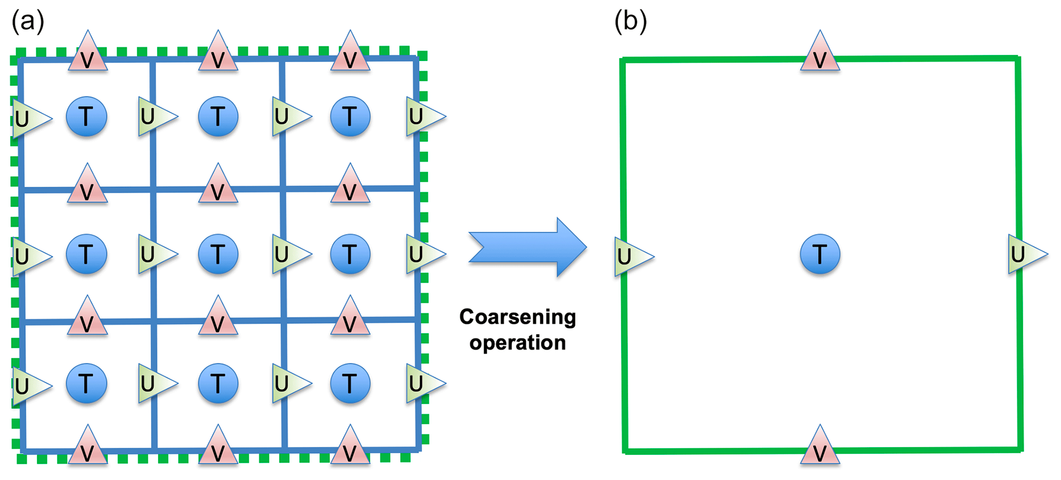
Figure 1Schematic diagram illustrating the definition of the coarsened grid for a coarsening factor of 3 (ocean high-resolution grid is in panel a; coarsened grid for biogeochemical model is in panel b) and localization of tracer (T, blue dots), zonal velocity (U, green triangles) and meridional velocity (V, red triangles) points in both grids. Grid sections that are common to both grids are coloured in green.
3.1.2 Horizontal dimensions
Defining the horizontal dimensions of the coarsened grid cells is necessary to compute gradient or divergence operators.
For a coarsening factor of 3, HRCRS zonal cell size is computed by summing three consecutive HR zonal cell sizes along the zonal direction, and HRCRS meridional cell size is computed by summing three consecutive HR meridional cell sizes along the meridional direction (Fig. 2).

Figure 2Horizontal dimensions of high-resolution ocean HR grid cells (blue lines, red arrows, with names following NEMO nomenclature) and the corresponding coarsened biogeochemical HRCRS grid cell (green lines).
3.1.3 Land–sea mask
Defining the land–sea mask for HRCRS is the most strenuous task of the multi-grid algorithm, which requires ad hoc verification as it can lead to substantial errors in the final outputs. If there is at least one ocean T point in the HR 3×3 pad, then the corresponding HRCRS T point will be considered as ocean, which can be defined automatically (Fig. 3, top panel). At the interface between two coarsened grid cells, we carefully retain the shape of the HR mask by adjusting the mask at U or V points: when there is at least one ocean point in the HR interface (as in Fig. 3 middle panel), then the interface of the HRCRS corresponding cells is defined as in the ocean. On the contrary, even if the two HRCRS T points are in the ocean, the interface between them may be defined as on the land, in the event that the corresponding HR points along the interface are all on land (Fig. 3, bottom panel).

Figure 3Schematic diagram illustrating the definition of land–sea mask from high-resolution ocean grid cells (a, blue lines with land cells filled in black) to the corresponding coarsened biogeochemical grid cells (b, green lines, with numbers identifying whether the corresponding point, here T or U, is defined as land (0) or ocean (1)).
3.1.4 Vertical dimensions
The vertical dimension of cells at T points (usually named e3t in NEMO) are used in vertical divergence and Laplacian operators throughout the biogeochemical code. For the divergence operator, it is important that the coarsening procedure preserves the HR grid volume. Hence, the vertical dimension of HRCRS grid cells e3tHRCRS is defined as the sum of the volume of the corresponding HR grid cells divided by the HRCRS grid cell horizontal surface area:
as illustrated in Fig. 4c. Note that we assume that HR grid points which are land masked have their vertical dimension equal to 0.
For the vertical gradient operator, the coarsening procedure must preserve the HR grid thickness. Therefore, we define another vertical dimension for HRCRS grid cells, e3tmax, as the maximum of the vertical dimensions of the corresponding HR grid cells:
as illustrated in Fig. 4d.

Figure 4Schematic diagram illustrating the coarsening procedure for the vertical dimension (e3t) of grid cells from high-resolution ocean grid cells (blue lines, a, b) to the corresponding coarsened biogeochemical grid cells (green lines, c, d).
3.2 Definition of coarsening operators
Once the coarser grid variables have been defined, the second step of the multi-grid algorithm consists of defining the operators used to coarsen the dynamic fields necessary to solve the passive transport equation.
3.2.1 Coarsening of state variables
In order to preserve conservation properties through coarsening operations, the intensive state variables (temperature, salinity) of the hydrodynamic model are coarsened such as their volume integrated quantities is the same on the finer and coarser grid. Therefore, the operator is a weighted mean over the 3×3 pad of HR cells corresponding to each HRCRS cell, where the weights are defined as the volume of the HR grid cells:
In order to preserve the non-divergence of velocities on the coarser grid, HRCRS velocities are computed so as to conserve horizontal fluxes at the edges of the cells. Hence, the horizontal velocities are coarsened using a weighted mean along the edges of the 3×3 pad of HR cells corresponding to each HRCRS cell, where the weights are defined as the area of the vertical faces of the HR grid cells:
where e12HR=e2uHR, e3xHR= e3uHR and l=j for zonal velocities, and e12HR= e1vHR, e3xHR= e3vHR, and l=i for meridional velocities. Note that it is the effective horizontal velocities that are coarsened to HRCRS, i.e. including eventual subgrid-scale parameterizations rather than the Eulerian velocities.
Vertical velocities and surface fluxes are coarsened using a weighted mean over the 3×3 pad of HR cells corresponding to each HRCRS cell, where the weights are defined as the horizontal area of HR grid cells:
3.2.2 Quantities related to the equation of state
Quantities related to the equation of state have a substantial impact on the model stability, via stratification. Therefore, it is necessary to define conscientiously the coarsening procedure of those, so as to prevent the multi-grid algorithm from generating spurious numerical instabilities.
The N2 buoyancy frequency in the HRCRS domain is computed by coarsening the HR N2 buoyancy using the mean operator (Eq. 6), a solution that is considerably cheaper than computing HRCRS N2 in the HRCRS domain. In parallel, the density in the HRCRS domain is computed from the temperature and salinity fields in the HRCRS domain. Finally, both the buoyancy frequency and density in HRCRS domain are used to compute the HRCRS slopes for neutral surfaces R. This ad hoc solution (note that there is no well-defined coarsening operator for a slope) was found to yield less numerical instabilities than others.
3.2.3 Subgrid-scale vertical processes
Vertical processes affecting passive tracers are predominantly led by vertical mixing are thus very sensitive to its amplitude. The vertical mixing coefficient Av has minimal background values on the order of m2 s−1 or less but can reach up to 10 m2 s−1 or more at sporadic grid points (when static instability occurs and the parameterization for convection is activated, for example). As a consequence, using a simple weighted mean of the HR Av as coarsening procedure is expected to be inappropriate. Indeed, with such a method, HRCRS Av would be exclusively reflecting occurrences of strong values of HR Av whether they are adjacent to lower ones or not. Henceforth, we define six different operators to coarsen the vertical mixing coefficient and test the sensitivity of the multi-grid algorithm to those (see Sect. 5.3.1):
-
the min and max operators, where the coarsened Av is the minimum or, respectively, the maximum of the HR Av over the 3×3 pad of HR cells corresponding to each HRCRS cell;
-
the mean operator, where the coarsened Av is computed by a weighted mean in a 3×3 pad of HR Av (i.e. the method expected to be inappropriate);
-
the median operator, where the coarsened Av is the median value in a 3×3 pad of HR Av; and
-
the meanlog operator, where the coarsened Av is computed by a weighted mean in logarithmic space in a 3×3 pad of HR Av.
3.3 Practical implementation in the NEMO ocean model
By default (i.e. without using the multi-grid algorithm), the model passive transport component uses the grid and dynamic variables computed by the dynamic component of the code (i.e. on the HR grid). It is necessary to implement the multi-grid algorithm for passive tracer transport in the NEMO ocean general circulation model (OGCM) without cancelling the default option. We describe here how the model passive transport component can switch to the HRCRS grid and dynamic variables when the multi-grid algorithm is activated.
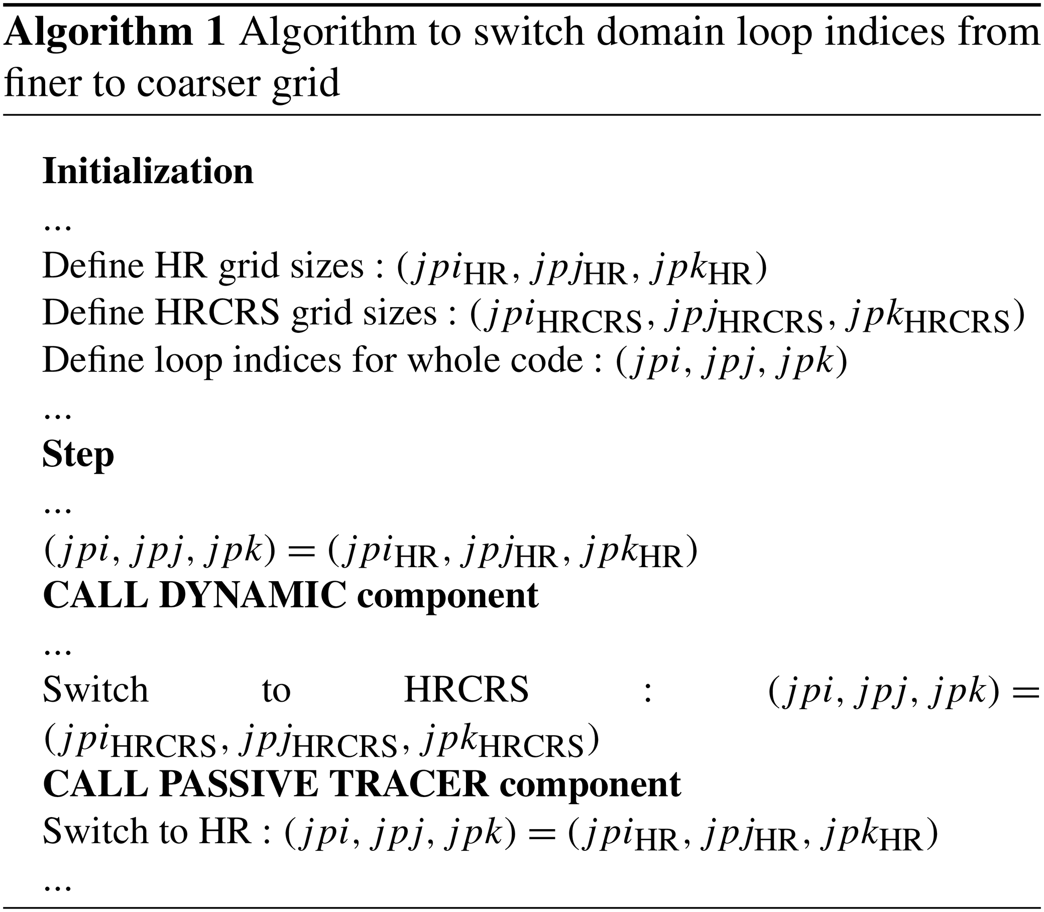
First we present how we manage the domain loop indices. The loops in the ocean dynamic and passive
transport components use the domain sizes in the three spatial directions (called
in NEMO). When the multi-grid algorithm is activated, HR grid sizes
are saved in other variables
and HRCRS coarsened grid sizes are
defined as . When the code is
in the ocean dynamic component, the loop sizes are
set to HR grid sizes . When the code enters the passive transport component, the loop sizes switch to HRCRS grid sizes
; when the code goes out of
the passive transport component, the loops sizes
switch back to HR grid sizes:
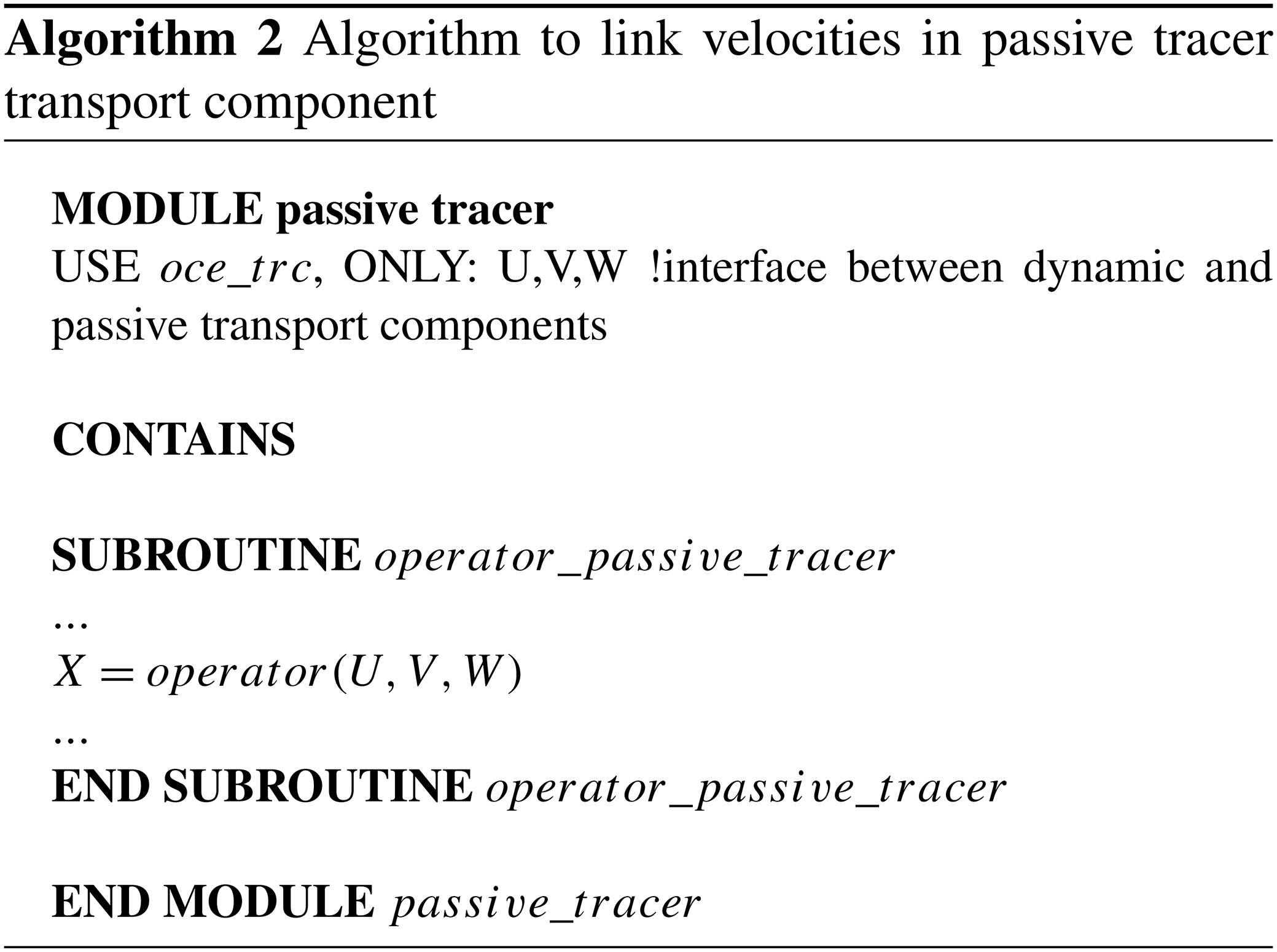
Secondly, we present how we manage the grid and dynamic variables used in the
passive transport component. They are made available through pointers
defined in an interface between the dynamical and passive transport
components (called oce_trc in NEMO OGCM):
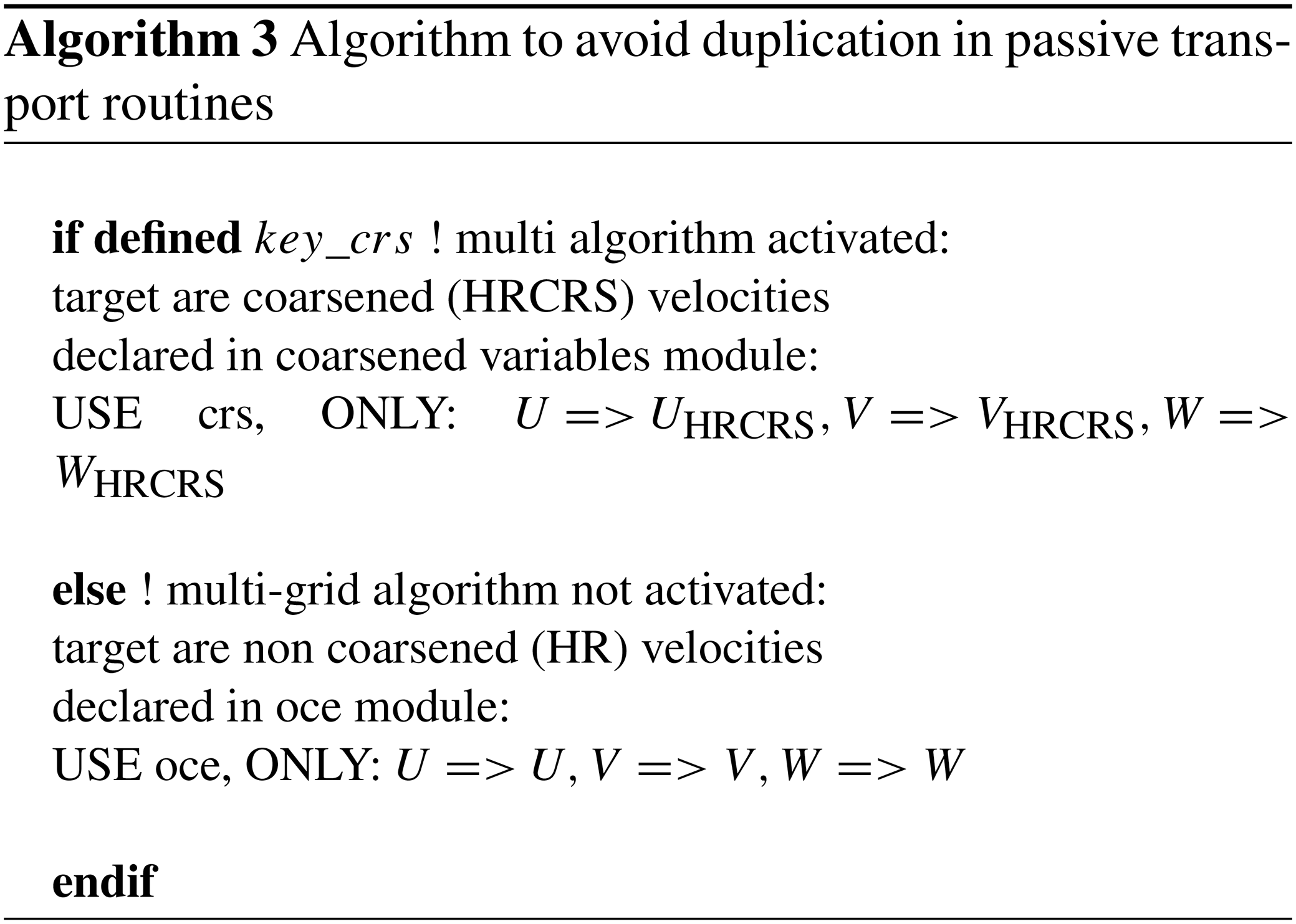
To avoid the duplication of coarsened and non coarsened grid and dynamic
variables in the passive transport routine, the pointers target the
coarsened grid and dynamic variables when the multi-grid algorithm
is activated and the non coarsened variables when it is not activated.
The choice between the two definitions is done at the pre-compilation
stage of the code with a cpp key key_crs:
The multi-grid algorithm has been implemented in NEMO OGCM (Madec et al., 2017) version 3.6 in which the OPA (Océan Parallélisé) ocean model is coupled to the Louvain-La-Neuve sea ice model (LIM) v3 (Rousset et al., 2015; Vancoppenolle et al., 2009) and its passive tracer transport component TOP (Tracer in the Ocean Paradigm).
Three different global ocean configurations have been employed to assess the multi-grid algorithm:
-
The first is the HR configuration, where the ocean hydrodynamic (i.e. open ocean and sea ice) and the passive tracer components are both running at resolution. This is the reference experiment using the highest possible resolution and no multi-grid algorithm for passive tracers.
-
The second configuration is the LR configuration, where the ocean hydrodynamic and the passive tracer components are both running at resolution. This experiment provides insights on the impact of horizontal resolution with still no multi-grid algorithm for passive tracers.
-
The third configuration is the HRCRS configuration, where the ocean hydrodynamic component is running at resolution, while the passive tracer is running at resolution. This experiment corresponds to the standard use of multi-grid algorithm for passive tracers.
It is important to state that it is not expected that the HRCRS configuration yields exactly the same results as the HR or LR configurations. Indeed, as there is some information missing in the coarsening procedure of ocean hydrodynamics from HR to HRCRS, the passive tracer distribution in HRCRS is not expected to be strictly the same as that in HR configuration. On the other hand, because the hydrodynamics in LR is running at coarser resolution than that in HRCRS, it is not expected that the passive tracer distribution in HRCRS is the same as that in LR. Yet, the multi-grid algorithm will be proven useful if the results of HRCRS are closer to HR than those of LR. Hence, the present experimental protocol should not be seen as a direct validation of the multi-grid algorithm but rather as an assessment of its potential benefits and limitations.
4.1 Model configurations
The configuration is described in Barnier et al. (2006). The configuration coordinates and bathymetry are built by applying configuration coordinates and bathymetry on the coarsening operators described above. This operation has created some fake straits in Panama and the Indonesian Throughflow, which have been manually filled. The configuration is close to the global ocean ORCA 1∘ configuration used in various Coupled Model Intercomparison Project phase 5 (CMIP5) (Voldoire et al., 2013) and CMIP6 models (Voldoire et al., 2019).
The and resolution configurations are based on a quasi-isotropic ORCA grid (Madec and Imbard, 1996) at nominal and horizontal resolutions, respectively, at the Equator. Vertical discretization uses 75 z levels with partial cell parameterization (Barnier et al., 2006), which leads to a resolution ranging from 1 m at the surface to 450 m at depth.
The bathymetry is based on a combination of ETOPO1 (Amante and Eakins, 2009) and GEBCO08 (Becker et al., 2009). The initial state for the ocean is at rest, with temperature and salinity from WOA13 (World Ocean Atlas; https://www.nodc.noaa.gov/, last access: 10 June 2015). At the surface, the model is forced by ERA-Interim atmospheric reanalysis (Dee et al., 2011) using the CORE bulk formulae Large and Yeager (2009) to compute the turbulent air–sea fluxes. A monthly runoff climatology is built and applied to all configurations, using data for coastal runoffs and major rivers from Dai and Trenberth (2002).
A split-explicit time-splitting scheme is employed to compute the surface pressure gradient with a non-linear free surface (Levier et al., 2007). These parameterizations were already used in the Ireland–Biscay–Iberia regional configuration, described in Maraldi et al. (2013).
The momentum advection term is computed with the energy and enstrophy conserving scheme proposed by Arakawa and Lamb (1981). The advection of tracers (temperature and salinity) is computed with a total variance diminishing (TVD) advection scheme (Lévy et al., 2001; Cravatte et al., 2007).
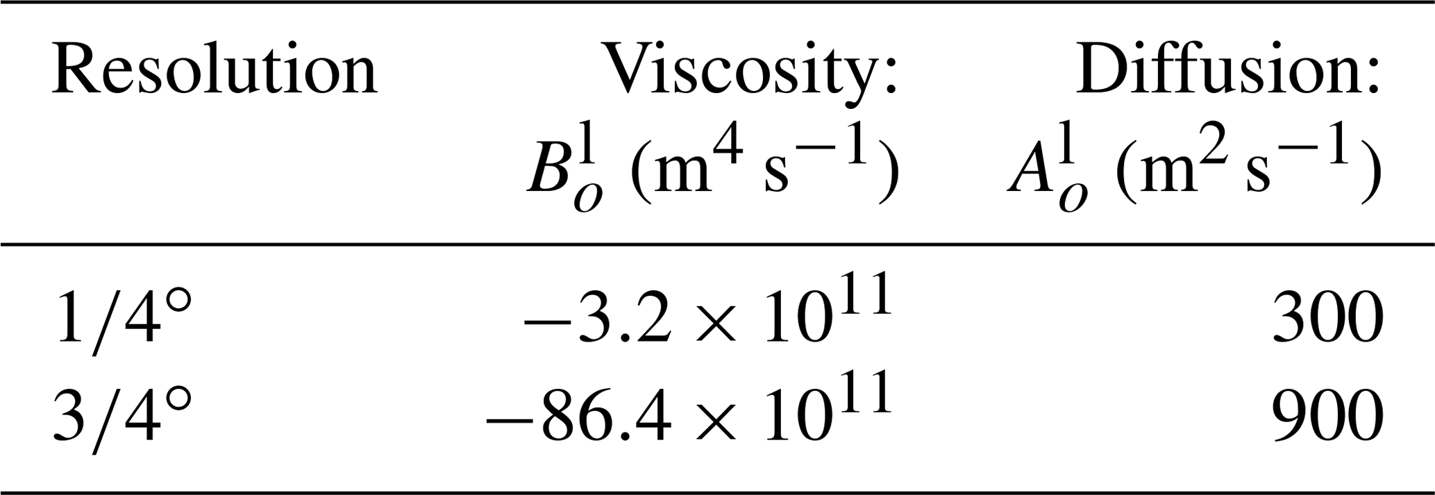
Lateral eddy viscosity is computed with a biharmonic operator and lateral eddy diffusivity is computed with an isopycnal Laplacian operator for both active and passive tracers. As explained in Madec et al. (2017) (Sect. 9.1), lateral eddy diffusivity coefficient Al decreases proportionally to the grid size, while the lateral eddy viscosity coefficient Bl decreases poleward as the cube of the grid cell size:
where and are the respective values at the Equator (see Table 1), while emax is the maximum of e1 and e2 taken over the whole masked ocean domain located at the Equator for global configurations. The lateral eddy diffusivity coefficients shown here are used for active tracers when the multi-grid algorithm is activated or not, and used for passive tracers when the multi-grid algorithm is not activated; the choice of lateral eddy diffusivity for passive tracers when the multi-grid algorithm is activated is discussed later (Sect. 5.2).
Table 1Horizontal eddy viscosity and diffusivity values at the Equator.
The vertical eddy viscosity and diffusivity coefficients are computed from a turbulent kinetic energy (TKE) turbulent closure model (Blanke and Delecluse, 1993), with parameters as described in Reffray et al. (2015).
4.2 Numerical experiments
To assess the multi-grid algorithm for passive tracers, three types of experiments have been set up. They differ on the passive tracer initial state or evolution. In all cases, the dynamical component is the same. The comparisons of the simulated tracer distributions are performed after 365 d of integration. At this stage, tracer fields have been transported and stirred during several mesoscale eddy turnover timescales, although tracer distributions are still far from statistical equilibrium.
In the PATCH experiments, the multi-grid algorithm is assessed on the horizontal component of the transport (Eq. 1). Here, the passive tracer vertical diffusivity component is set to 0 . The passive tracer C is initialized with a patch of 10∘ radius centred on 36∘ N, 60∘ W (see Fig. 6a). The value of the tracer ranges from 2 at its center to 1.368 at its boundaries and is vertically uniform. Outside of the patch, the tracer initial value is set to 1. The tracer has no sources nor sinks. Hence, the passive tracer evolution in the PATCH experiment can be described by the following equations:
where R is a tensor of isoneutral slopes.
The AGE-ZDIF experiments (AGE for age tracer; ZDIF for vertical diffusion) are conceived to assess the multi-grid algorithm on the vertical eddy diffusive component of the passive tracer transport (Eq. 1). Hence, the advection and lateral diffusion are unplugged for the passive tracer. This experiment makes use of the so-called age tracer of the NEMO OGCM: its initial value is set to zero in all the ocean and its value is damped to 0 at the ocean surface, while there is a net source in the ocean interior. This tracer gives a good representation of the time evolution of a water mass after it was in contact with the ocean surface; hence, it gives some information on the ventilation of water masses. The tracer evolution in the AGE-ZDIF experiment can be described by the following equations:
Finally, the multi-grid algorithm is assessed on the full tracer transport (Eq. 1) in the AGE-FULL experiment (FULL for full equation), which also uses the age tracer but retains all terms for the tracer transport equation. Hence, the tracer evolution in the AGE-FULL experiment can be described by the following equations:
5.1 Coarsened velocities
Advection by ocean currents is one of the main drivers of the evolution of passive tracers. As a consequence, it is important that tracer transport by ocean currents on the coarsened grid HRCRS remains close to that on the HR grid. This implies that coarsened velocities share similarities with HR velocities on the spatial scales that are common. To test this, coarsened velocities are compared to HR velocities and LR velocities (Fig. 5), as done by Lévy et al. (2012) in a more idealized context. Power spectra are computed along the horizontal coordinates of the model grids. For each spectrum, the minimum wavelength corresponds to twice model grid spacing: 2⋅Δx. HRCRS velocities are the result of the coarsening of HR velocities on LR grid. As HR grid is finer than LR grid, HR velocities contains finer scales than HRCRS and LR.
In terms of kinetic energy, vertical velocities and relative vorticity, HR, HRCRS and LR have almost the same level of energy at spatial scales larger than 250 km. At smaller spatial scales, HRCRS has a level of energy comparable to HR in terms of kinetic energy and relative vorticity, while vertical velocities are less energetic than in HR. For the three quantities, at spatial scales smaller than 250 km, the level of energy of LR is significantly below HR and HRCRS levels. This suggests that ocean currents in HRCRS are, overall, more similar to those in HR than to those in LR.
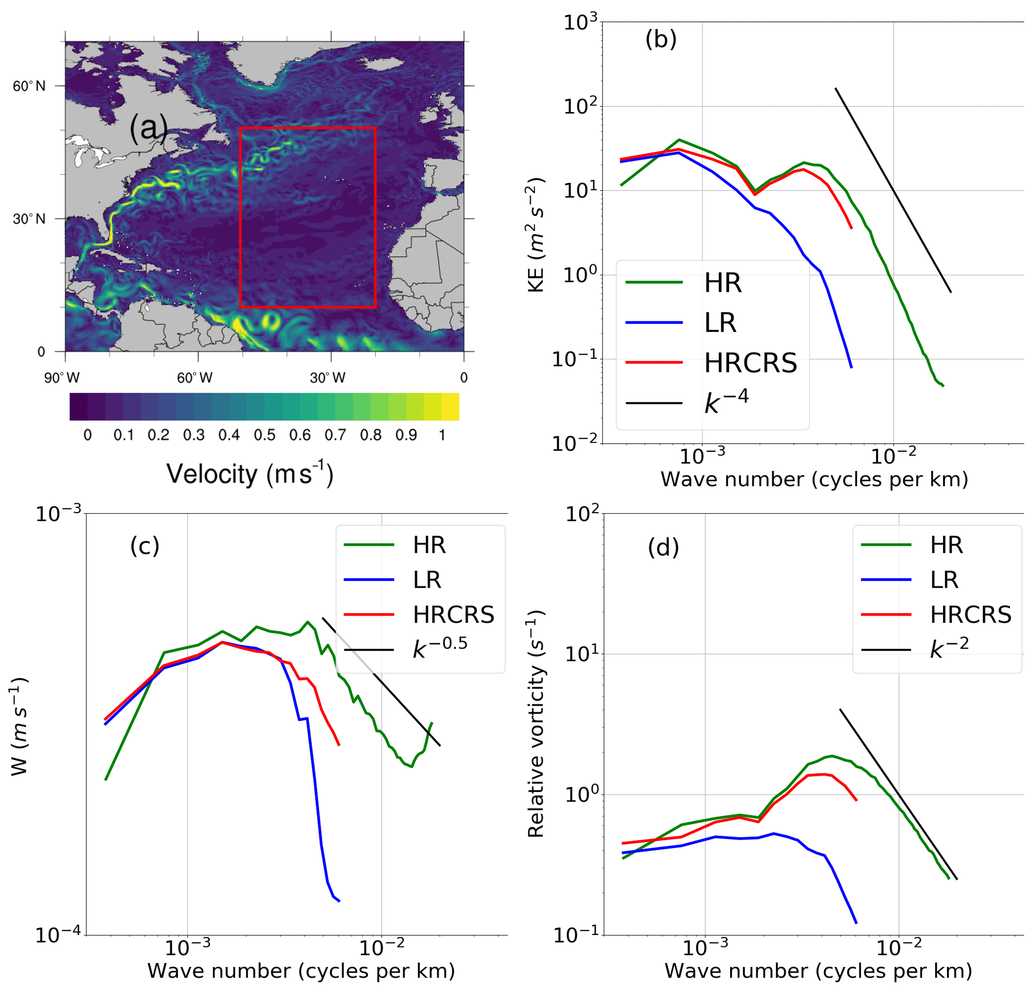
Figure 5North Atlantic yearly mean surface current speed (a) and power spectrum density of (b) surface kinetic energy, (c) vertical velocities and (d) surface vorticity as functions of spatial wave number, in the HR (green lines), LR (blue lines) and HRCRS configurations (red lines). Black lines in spectra represent usual slopes to be compared with numerical spectra. All computations use daily model outputs and are averaged yearly.
5.2 Horizontal tracer transport
The evaluation of the multi-grid algorithm to resolve an advection–diffusion problem is shown here with the results of the PATCH experiment described in Sect. 4.2.
The first step is to evaluate the best value for the passive tracer horizontal diffusion coefficient in the HRCRS configuration. A comparison between HR and various HRCRS configurations differing for their horizontal diffusion coefficient (set to 300, 600, 900 and 1200 m2 s−1) is presented in Sect. A. This sensitivity test suggests that 900 m2 s−1 yields the best results for HRCRS. Using 300 m2 s−1 in HR and 900 m2 s−1 in HRCRS for the passive tracer lateral diffusion respects the ratio in spatial resolution between the two configurations (of respectively and nominal resolution), which is consistent with the linear relationship between the horizontal diffusion coefficient Al and the cell size (see Eq. 9).
Using this value for the lateral diffusion coefficient Al in the HRCRS configuration, and comparing outputs to those from HR and LR configurations, suggests that the HRCRS patch is closer to the HR shape than to the LR one (Fig. 6). Indeed, LR has a larger area where its concentration is higher than in HR, with a difference greater than 0.3 in its center, while the difference between HRCRS and HR does not exceed 0.2 (within the red box, after 1 year of simulation; the root mean square error (RMSE) is 0.04 between HRCRS and HR and 0.09 between LR and HR).
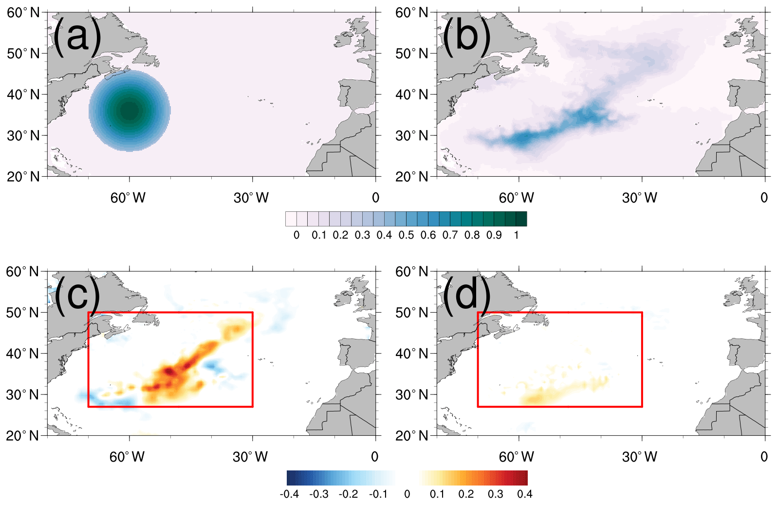
Figure 6Passive tracer initial condition for PATCH experiment (a), tracer concentration at 16 m depth after 1 year for the HR configuration (b) and difference with LR (c) and HRCRS configurations (d), respectively.
Horizontal velocities influence the interior EKE distribution and so the tracer distribution. In Fig. 7, we represent for a meridional section in the Gulf Stream the daily vertical distribution of zonal velocities and PATCH tracer after 1 year of simulation, for the HR, HRCRS and LR configurations. The HRCRS velocities are obtained by coarsening the HR velocities. HR and HRCRS zonal velocities are stronger than LR velocities and present more fine structures, in particular in the northern region (above 40∘ N). HRCRS and HR tracer distribution are similar and present some differences to LR configuration. In the southern part of the 55∘ W sections, LR configurations has a maximum of concentration, whereas HRCRS and HR have lower values. In the northern parts of the section, HR and HRCRS have some higher values of concentration in the interior and deeper ocean than in LR configuration, around 40∘ N latitude. Despite the degraded spatial resolution operated on the velocities, the dynamics used to transport HRCRS tracer present the same pattern as the HR dynamics. The tracer using the multi-grid algorithm reproduces the HR tracer; while the dynamics is coarsened, the HRCRS tracer benefits from the higher-resolution dynamics and present a gain compared to a lower-resolution experiment.

Figure 7Vertical distribution of the zonal velocities (m s−1) (a, b, c) and PATCH tracer (d, e, f) for HR (a, d), HRCRS (b, e) and LR (c, f) configurations along the 55∘ W section in the Gulf Stream.
5.3 Vertical diffusion
5.3.1 Choice of vertical diffusion on the coarsened grid
Vertical mixing is responsible for the ventilation of a passive tracers and thus their vertical distribution. The vertical diffusion coefficient Av is computed by the dynamic component (so on the HR grid) but it might be coarsened on the HRCRS grid.
Here, we present the results of the AGE-ZDIF experiment in order to assess the capacity of the multi-grid algorithm to simulate the passive tracer vertical mixing. In particular, we show the sensitivity of the age tracer vertical representation to the choice of coarsening operator of the vertical mixing parameter Av presented in Sect. 3.2.4.
Figure 8a–b present the daily vertical profiles of root mean square (rms) difference to the HR age tracer after 1 year of simulation. All the configurations have the same shape of vertical distribution, except LR and HRCRS with the max operator which have a behaviour very different to the others at the bottom of the ocean. Figure 8b presents a zoom in the first 500 m. All the configurations have some differences in the mixed layer and some HRCRS configurations are closer to HR, according to the coarsening operator used for the vertical mixing: the HRCRS with the meanlog and median operators give the best performance compared to the HR experiment, whereas the HRCRS experiments with the two extreme operators give results less comparable to LR.
Table 2 gives the RMSE with the HR solution for all HRCRS experiments and LR. The HRCRS with meanlog and median operators gives the best results. HRCRS with min and HRCRS with mean have a better skill than LR, and HRCRS with max is far from the other simulations.
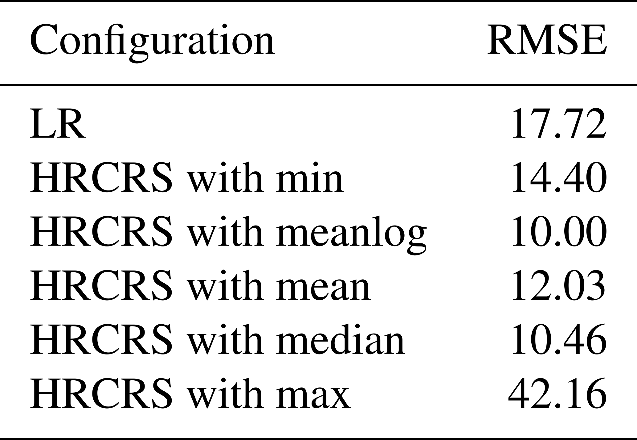
To understand which process leads to these solutions, we present in Fig. 8c–e the divergence of the age tracer vertical diffusive fluxes averaged over the global ocean and the first year of the simulation. A positive divergence means that the net incoming fluxes are positives. Looking at the flux to the bottom (Fig. 8e) shows that the divergence is negative for HRCRS with the max operator; it is coherent with the fact that age tracer concentration is lower than the other (see Fig. 8a). It is explained by the fact that the max operator extends the zone where the Av has a high value along the bathymetry. HRCRS with the min operator has a negative flux divergence at the bottom, but its age value is closer to HR.
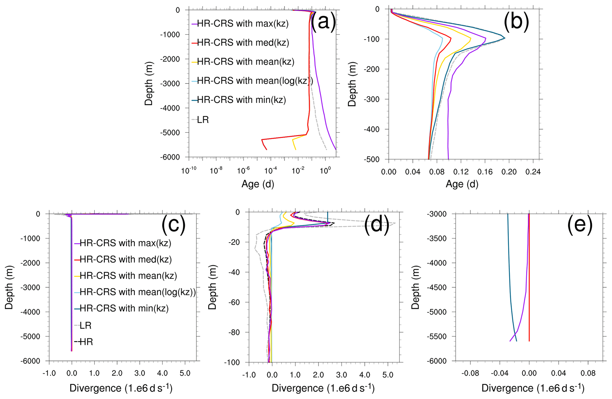
Figure 8(a, b) The rms differences to HR age tracer for HRCRS and LR runs for the whole water column (a) and for the first 500 m (b). The age tracer values are instantaneous outputs after 1 year. (c–e) Horizontal mean of divergence of age tracer vertical diffusive flux mean over the first year for the whole water column (c), the top ocean (d) and the bottom ocean (e).
5.3.2 Special case for convection
Here, we assess the multi-grid algorithm at simulating the age tracer penetration for deep convection as in the Ross and Weddell seas. We want to know if the operators selected in the previous section (meanlog and median) are appropriate for this particular situation.
Figure 9 represents the depth where the age tracer reaches the value of 10 d (Fig. 9a–b) and 100 d, along a section in the Southern Ocean, at the latitude of 58.3∘ S. In Fig. 9a and c, we compare the HR profile (black), the LR experiment (grey) and the ensemble spread of the different solutions of HRCRS (light blue). The HR profile is included in the HRCRS ensemble, whereas the LR experiment is outside of the HRCRS spread. All the HRCRS solutions have better performance than the LR solution compared to HR. However, the spread is larger in two areas: between 140 and 80∘ W and between 100 and 160∘ E.
Figure 9b and d show the differences between each HRCRS solutions and HR. We can see that, outside of the two areas of deep convection, the HRCRS solutions performed with the meanlog and median operators are the closest to the HR solution, especially in the deeper case (Fig. 9d). Around 100∘ E and 150∘ W, the HRCRS solution with the min operator is the closest to HR solution.
In order to combine the better performance of the min operator in the convection situation and the meanlog operator in the global ocean, we add here a new operator based on the meanlog operator with a switch to the min operator in presence of convection. The HRCRS run with the meanlog operator and a switch to the min operator gives the best comparison to the HR run in the Weddell and Ross Sea areas and has good performance outside.

Figure 9Antarctic Circumpolar Current (ACC) section ( S) of depth where age tracer value is equal to a given age: 10 d (a, b) and 100 d (c, d). Panels (a) and (c) compare HR, LR and the mean of HRCRS runs. Panels (b) and (d) show the difference between HR and all the HRCRS runs.

Figure 10Depth where age tracer is equal to 100 d after 1 year of simulation: HR experiment (a), LR minus HR (b) and HRCRS minus HR (c).
5.4 Evaluation of the full algorithm
We have validated the multi-grid algorithm to represent the tracer advection and lateral diffusion in Sect. 5.2 and the vertical eddy diffusion in Sect. 5.3. The choice of the operator to coarsen the vertical diffusion coefficient Av has also been discussed in Sect. 5.3. Now we present some results for the full transport (Eq. 1). We decide to continue the assessment using the meanlog operator to coarsen the vertical diffusion coefficient.
A comparison of the depth for HRCRS and LR runs to HR run is presented in Fig. 10. Figure 10a presents the HR depths where age is equal to 100 d. Figure 10b presents the depth differences between LR and HR, and Fig. 10c presents the depth differences between HRCRS and HR. Higher depths values are due to deeper age tracer penetration, caused by higher vertical mixing. Globally, there are no big differences between the three runs, except in the area where mesoscale activity is important: the Gulf Stream, the North Atlantic subpolar gyre, the Kuroshio Current and the Southern Ocean. The differences between HRCRS and HR runs are largely weaker than the differences between LR and HR runs.
In order to compare on depth the three different runs, we present in Fig. 11 the age tracer penetration along three sections. The first section starts in the Antarctic Circumpolar Current (ACC) and goes northward until the North Atlantic. For a value of 10 d, the penetration for the three experiments are close. For a value of 100 or 300 d, HRCRS is very close to HR run and LR is different from the two other experiments. The second section goes along the equatorial Pacific. For the three values of the age tracer, the corresponding depths from HR and HRCRS are very close and the depths from the LR experiment are different. The last section is inside the ACC. HRCRS and HR depths are similar for 10, 100 and 300 d. LR run depths are similar to the two other runs for 10 d, and the differences with the two other runs increase with depth.
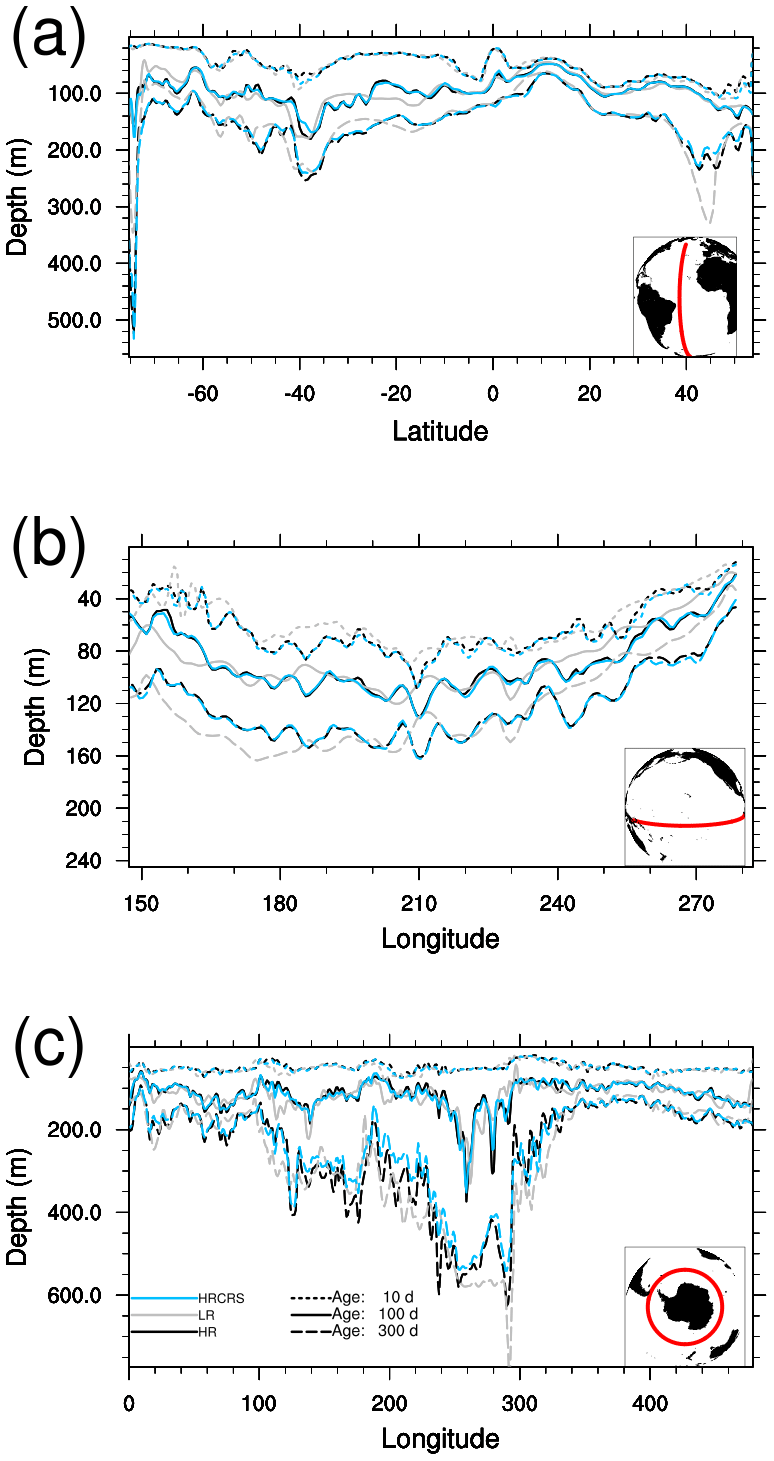
Figure 11Atlantic (a), Pacific (b) and ACC (c) sections of age tracers after 1 year of simulation for HR (black), LR (grey) and HRCRS (blue) configurations. The age value is 10 d (dotted line), 100 d (solid line) and 300 d (dashed line).
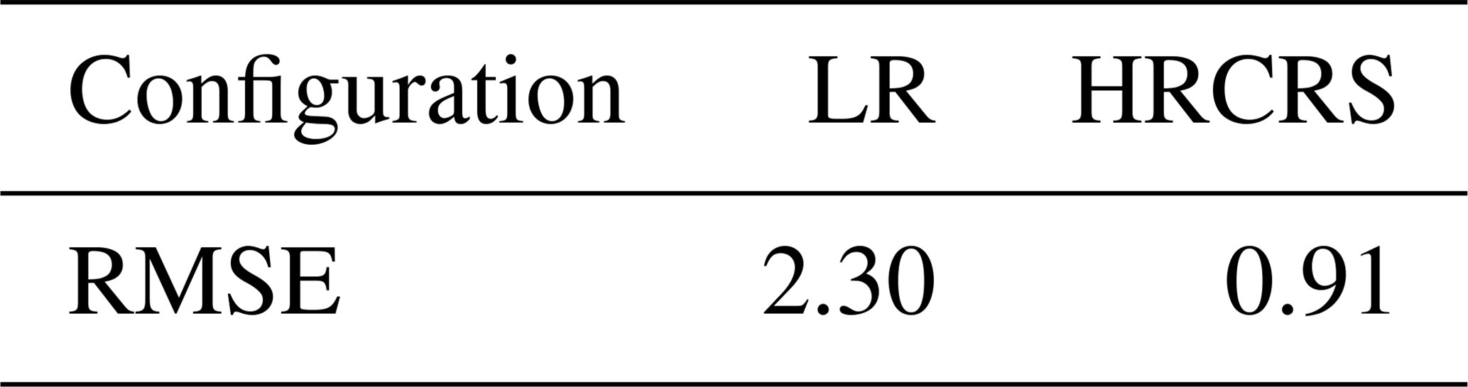
The age tracer RMSE with the HR solution has a value of 0.91 for HRCRS and 2.30 for LR after 1 year of simulation (Table 3).
5.5 Computational performance
Because of the extra computational cost of the coarsening of dynamical fields, the multi-grid algorithm procedure gives better performance only with large numbers of passive tracer fields. Indeed, the expected speed-up for computing tracer advection on a 3×3 coarser-resolution grid is a priori a factor of 9. However, in practice, the time spent on defining the grid and computing dynamical fields on the coarsened grid should also be accounted for. We present in Table 4 the elapsed time spent by the HR run (without grid coarsening capacity) and HRCRS run (with grid coarsening capacity). The elapsed time spent defining the scale factors for the coarsened grid and computing the dynamic fields on the coarsened grid is actually significant. This is why, for a single tracer field, the HRCRS run (with grid coarsening capacity) uses more CPU resources than the HR run. But it should be noted that the definition of the coarsened grid and the coarsening of dynamical fields are only done once for all the tracer fields. Therefore, the net overhead cost of this extra operation is relatively small in situations with many tracer fields (as shown in the last row of Table 4).
Table 4Elapsed time (in seconds) for a 1-month run without/with the multi-grid algorithm. The values in the last row have been extrapolated.
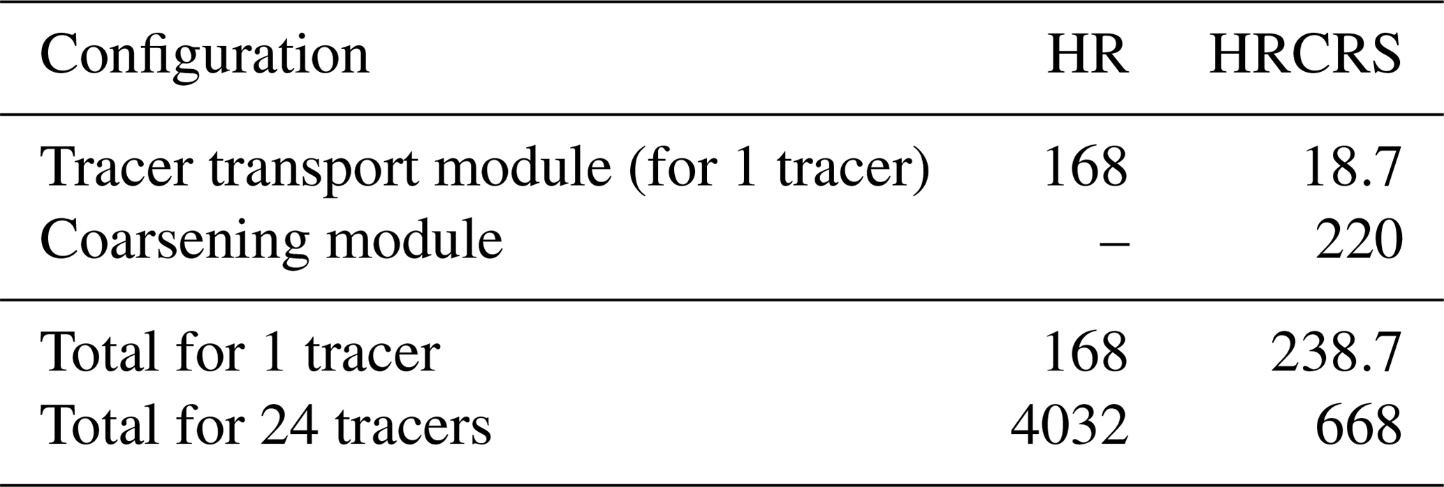
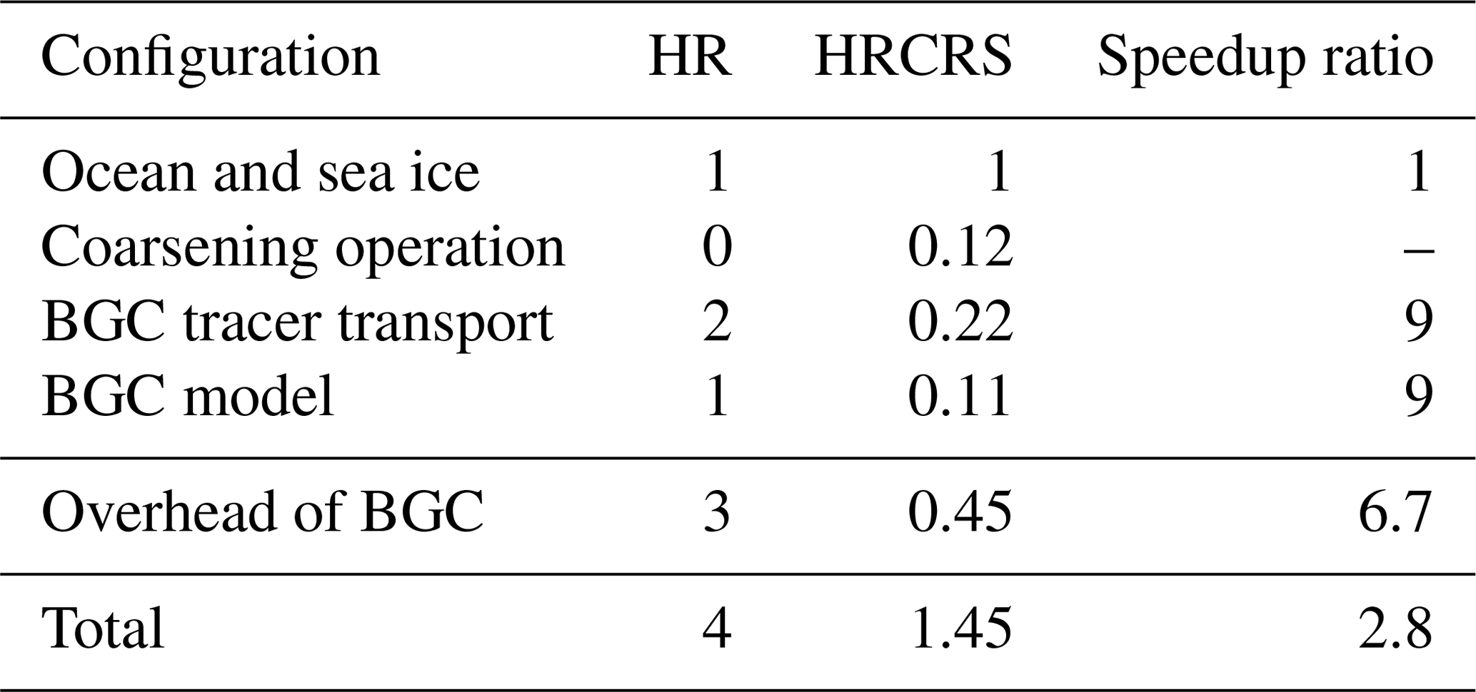
Overall, we estimate that using the multi-grid algorithm allows us to reduce the cost of running a full ocean model with an interactive biogeochemical component by a factor of ∼3. Table 5 provides an estimate of the breakdown of elapsed time in a global NEMO configuration coupled to PISCES biogeochemical model (Aumont et al., 2015), which simulates 24 passive tracers. Typically, running NEMO biogeochemical transport module (TOP) for 24 tracers on the same grid as the dynamics requires twice as much resources as the ocean–sea-ice component. PISCES biogeochemical component itself uses resources comparable to those used for the ocean–sea-ice component. Running a full model with a biogeochemical component based on PISCES typically requires 4 times the resources of the ocean–sea-ice component alone. Given the figures of Table 4, we estimate that the net elapsed time overhead of the biogeochemical component (transport + PISCES) would be reduced by a factor of ∼7 with the multi-grid algorithm. Therefore, a full model using our multi-grid algorithm would use 1.45 times more resources than the ocean–sea-ice component alone, therefore reducing the cost of the overall system by a factor of 3.
Table 5Typical expected speedup in elapsed time between a run without versus with multi-grid algorithm. Values have been extrapolated from the measured cost of the coarsening operation and an estimate of the net overhead of the PISCES biogeochemical (BGC) model.
A key limitation of the multi-grid algorithm described in this paper is its restriction to odd coarsening factors. As shown in Fig. 12, two possibilities would exist for defining an averaging procedure in the case of even coarsening factors but none of them would be fully amenable for defining a robust coarsening procedure. On the one hand, Fig. 12 shows that there is no obvious definition for lateral fluxes at the cell boundaries if the cell resulting from the averaging of several T cells is centred at a T point. On the other hand, a consistent treatment of north-fold boundary conditions in the HR and HRCRS grids requires that both grids share the same pivot point at the north-fold boundary (as described in Madec et al., 2017; see, in particular, their Fig. 8.4). This is why it is not possible to use an averaging procedure where the cell resulting from the averaging of T cells is centred at an F point.
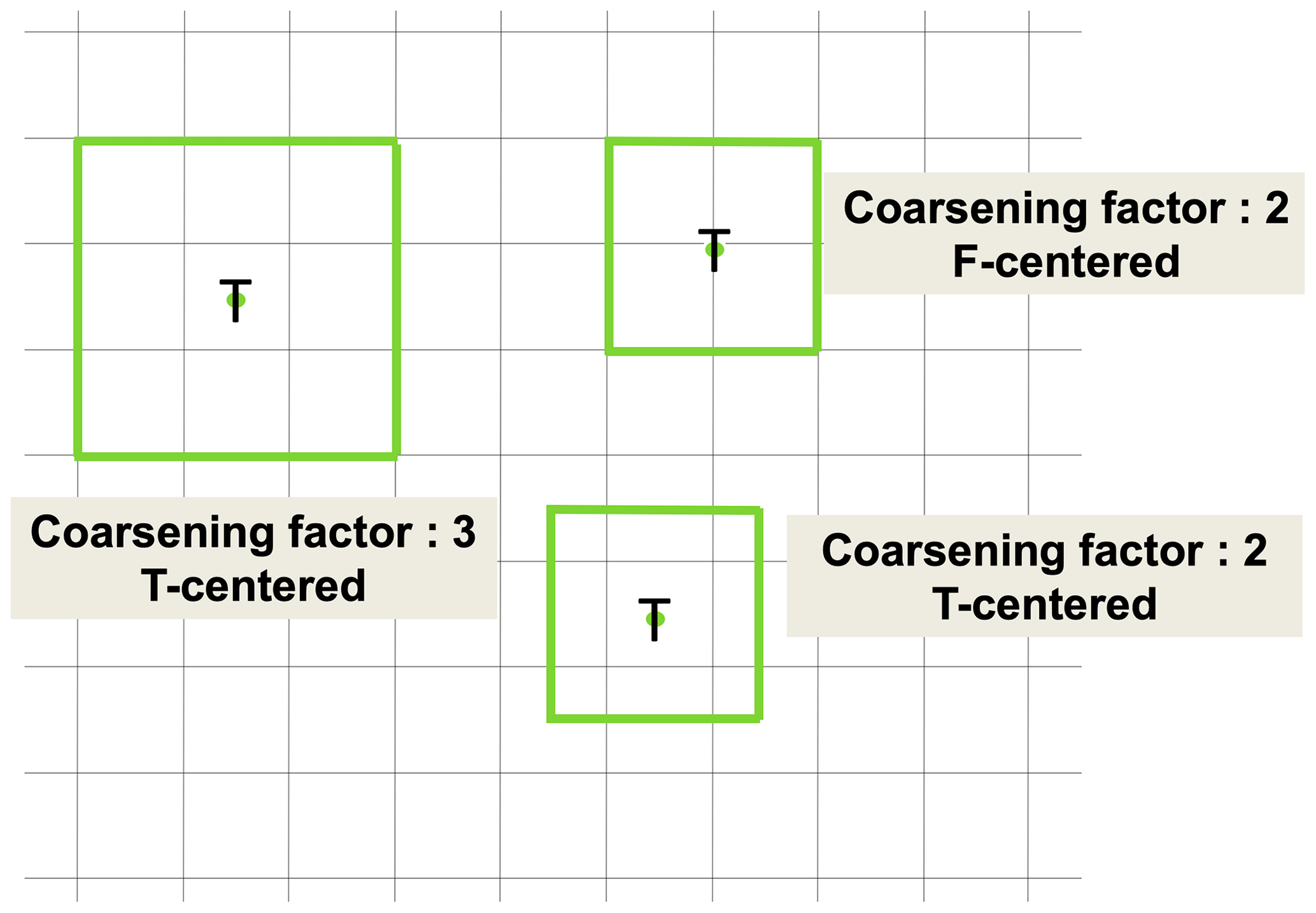
Figure 12Position of coarsened cells (green) on its high-resolution grid local mpp domain for some odd or even coarsening factors.
The present implementation is even more limited since only a coarsening factor of 3 is allowed. This limitation is related to constraints associated with multiprocessor applications. Indeed using a larger coarsening factor would require increasing the width of Message Passing Interface (MPI) overlapping areas (halo ghost cells for data exchanges with neighbouring processors). This is illustrated in Fig. 13, which shows that using a spatial coarsening factor of 5 would require extending the MPI overlapping area with an extra grid point in each direction. But, as for NEMO v3.6, the width of MPI overlapping areas is limited to one grid point in each direction.
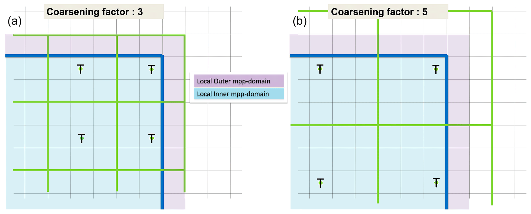
Figure 13Position of coarsened cells (green), on their high-resolution grid local mpp domain, for a coarsening factor of 3 (a) and coarsening factor of 5 (b).
A natural perspective of this work would be to add time subsampling. Indeed, in its present form, our multi-grid algorithm uses the same time stepping for both the HR and HRCRS grids. But the integration on the HRCRS grid could probably be carried out with a larger time step, which would further reduce the computational cost of tracer advection. As described in Sect. 3.2 of Madec et al. (2017) and in Leclair and Madec (2009), NEMO currently uses a leap-frog time-stepping scheme with a Robert–Asselin filter. In this context, extending our algorithm to the discretization in time is non-trivial because it would require keeping in memory several consecutive occurrences of the prognostic variables and grid cell volumes. Allowing time coarsening would be greatly simplified with a two-level time-stepping scheme in NEMO (which is planned for NEMO v5.0).
An algorithm based on multiple grids has been developed and implemented in the NEMO v3.6 ocean model for accelerating the integration of ocean biogeochemical models. The core of the algorithm is to compute the evolution of biogeochemical variables on a grid whose resolution is degraded by a factor of 3×3 with respect to the dynamical fields. We have described in detail the operators that allow the switch from the high-resolution (HR) grid to a coarser-resolution grid (HRCRS) and how to define optimally the evolution operators on the coarse grid based on information at high resolution. We have in particular described how several vertical-scale factors should be introduced and described the different options for the treatment of vertical physics on the coarse grid. A series of numerical tests performed under realistic conditions has been carried out for identifying how to optimally represent vertical mixing on the coarser grid.
The solutions computed with the full algorithm have been compared to solutions obtained using a high-resolution grid for both dynamics and passive tracers (HR configuration, resolution), and solutions were obtained using the lower-resolution grid for both dynamics and passive tracers (LR configuration, resolution) in a series of global ocean model experiments. We have shown that the proposed method provides solutions at global scale that are notably improved as compared to LR solutions and comparable to HR solutions. This confirms our working hypothesis that fluctuations of dynamical quantities close to the HR grid size have a negligible impact on tracer transport.
The evaluation of computational performance shows that the multi-grid approach does not reduce the computing time in the case of a single passive tracer because of the overhead associated with the definition and computation of dynamical quantities on the coarse grid. However, the reduction of elapsed time might be substantial when the algorithm is applied to multiple tracers as in the case of comprehensive biogeochemical models (an estimate has been provided but not proven). The proposed algorithm allows us to reduce by a factor of 7 the overhead associated with running a full biogeochemical model with 24 tracer fields in NEMO simulations.
Several possible directions for further improving the performance of the algorithm have been identified but they may require important changes to the NEMO code. Increasing the width of MPI overlapping areas in NEMO would allow us to increase the spatial coarsening factor (now limited to a factor of 3 in the present version). In addition, the use of more selective coarsening operators (Debreu et al., 2008) would bring the coarsened solution even closer to the uncoarsened solution. Their larger spatial stencil would however bring similar issues as for the coarsening factor limitation in a multi-grid processor environment. Extending our approach to the discretization in time is also a natural direction. Using a two-level time-stepping scheme instead of the leap-frog time-stepping scheme currently used in NEMO would greatly simplify such a development.
The algorithm we propose in this article makes it possible to run global applications of complex ocean biogeochemical models at eddying resolution over several decades. By reducing the computational overhead of running complex biogeochemical components in high-resolution ocean models, our algorithm opens the possibility to explicitly account for the impact of mesoscale ocean dynamics on ocean biogeochemistry in operational and climate models. The benefit of this approach in the context of climate modelling has recently been illustrated by Berthet et al. (2019).
In a coupled ocean–biogeochemical model, where the ocean and biogeochemical components are running at the same resolution, as the HR and LR configurations, the horizontal diffusion coefficient Al value is the same for active tracers (temperature and salinity) and the passive tracers (the biogeochemical tracers, or the PATCH tracer here). With the multi-grid capacity, passive tracers are running at a lower resolution than active tracers. We need to evaluate the best diffusion coefficient value for the passive tracers. Here, we present the results of the HR and HRCRS configurations for the PATCH experiment described in Sect. 4.2.1.
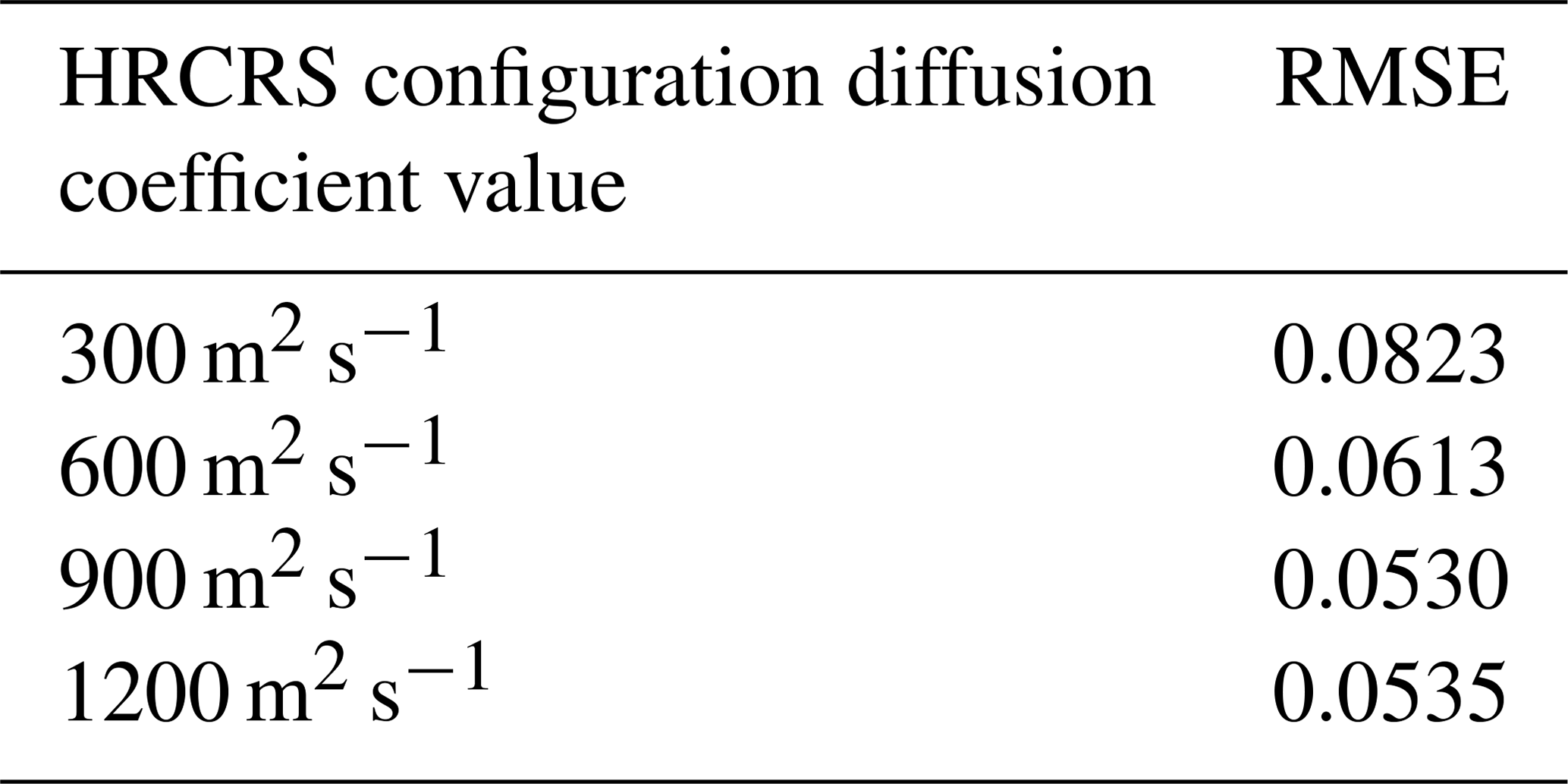
The reference diffusion coefficient value from Eq. (9) is 300 m2 s−1 for HR configuration and different simulations have been performed for HRCRS configurations with values of 300, 600, 900 and 1200 m2 s−1 for . Figure A1a represents the HR solution at its resolution. Differences of HRCRS solutions with HR are represented in Fig. A1b–e.
The HRCRS configurations runs with values of 300 and 600 m2 s−1 for seems to be too noisy compared to the HR configuration; the maximum value of the tracer inside the patch is also too high compared to HR configuration maximum. The HRCRS configuration run with a value of 1200 m2 s−1 for seems to be a little bit more diffuse compared to HR configuration and the maximum value is a little bit lower. The HRCRS configuration run with a value of 900 m2 s−1 gives the better reproduction to HR configuration in term of the patch distribution and fine-scale representation.
Table A1 gives the RMSE with HR for all experiments in the red box. The best result is obtained with a diffusion coefficient value of 900 m2 s−1 and the worst with a value of 300 m2 s−1. The results obtained with 1200 m2 s−1 are close to the best solution.
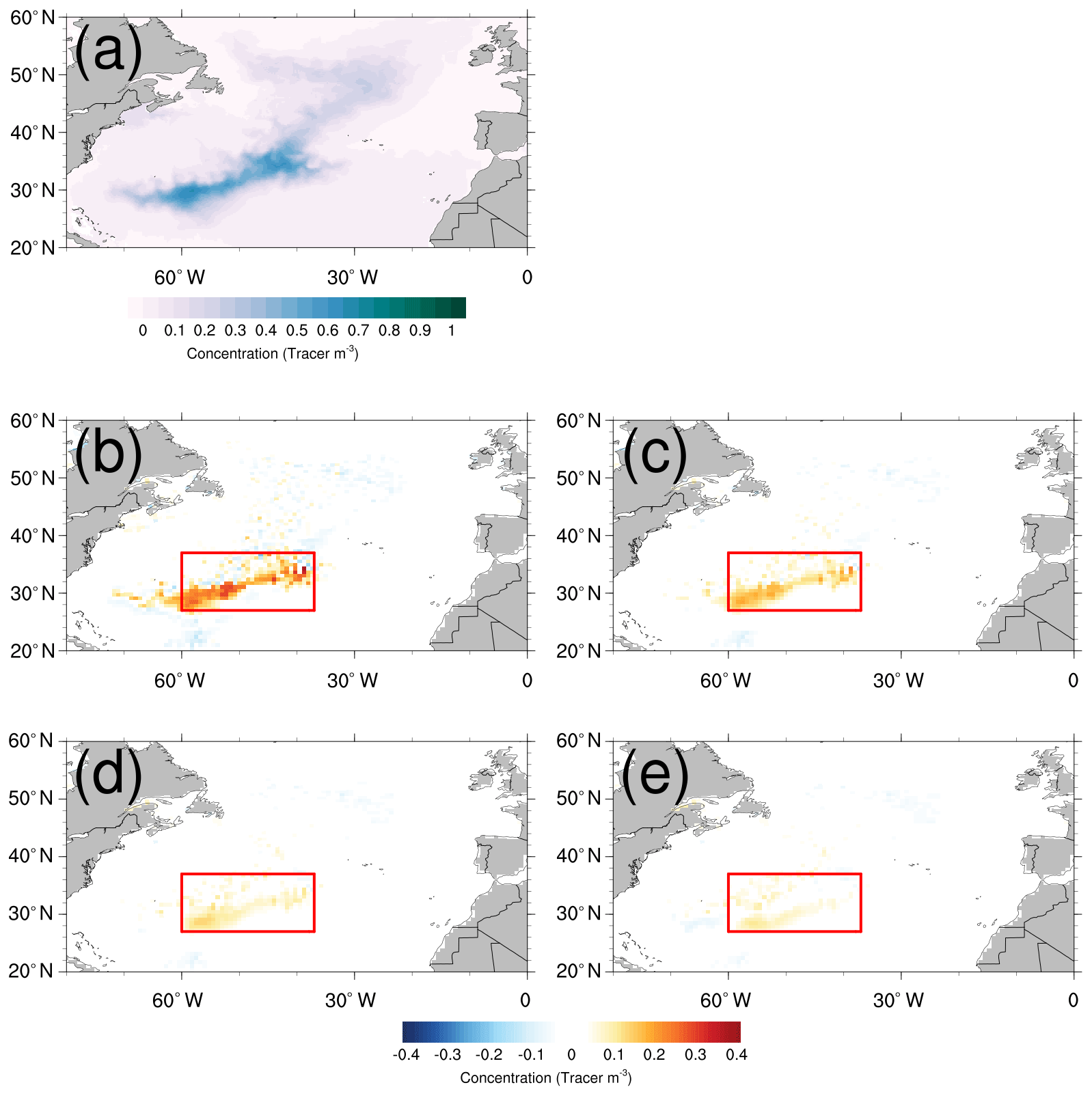
Figure A1Surface values of the patch tracer after 1 year for the HR configuration (a); differences between HRCRS and HR configurations with diffusion equal to 300 m2 s−1 (b), diffusion equal to 600 m2 s−1 (c), diffusion equal to 900 m2 s−1 (d) and diffusion equal to 1200 m2 s−1 (e).
The code containing the multi-grid algorithm has been developed in the NEMO OGCM framework (https://www.nemooceaneu/, last access: last access: 31 October 2020, NEMO System Team, 2020). This capacity is available on a development branch of the NEMO v3.6 stable release and is available after registration on NEMO forge (Bricaud, 2018), multigrid algorithm development branch, https://forge.ipsl.jussieu.fr/nemo/browser/NEMO/branches/2018/dev_r5003_MERCATOR6_CRS, last access: 26 October 2018). The NEMO source code is freely available and distributed under CeCILL license (GNU GPL compatible). The following cpp keys have been used to compile the code:
key_dynspg_ts, key_lim3, key_vvl, key_ldfslp, key_traldf_c2d, key_dynldf_c2d, key_zdftke, key_mpp_mpi, key_iomput, key_nosignedzero, key_top, key_my_trc and key_xios2.
The key_crs key is added to this list to activate the multi-grid algorithm.
The exact version of the model used to produce the results used in this paper is archived on Zenodo at https://doi.org/10.5281/zenodo.3615356 (Bricaud, 2020), as are input data and scripts to run the model and produce the plots for all the simulations presented in this paper.
The model outputs used in this paper are available at https://doi.org/10.5281/zenodo.3547421 (Bricaud, 2019).
CB, CC, GM and CE developed the model code. CB, JLS and JC designed the experiments. CB performed the simulations. CB and JLS prepared the manuscript with contributions from ML, JD and JC.
The authors declare that they have no conflict of interest.
The development of the multi-grid algorithm for passive tracers was supported by EU MyOcean and MyOcean2 projects, the EMBRACE project (European Union's Seventh Framework Programme for research under grant agreement no. 282672), then by the EU Copernicus Marine Environment Monitoring Service (CMEMS), the French ANR SOBUMS (ANR-16-CE01-0014) and the CMEMS 22-GLO-HR project. The development and the simulation shown in this paper have been produced on the ECMWF CCA Cray supercomputer.
This research has been supported by the Eu FP7 projects Myocean (grant no. 218812), EMBRACE (grant no. 282672) and Myocean2(grant no. 283367), the Eu CMEMS service (Copernicus European Earth Observation Programme) and the French ANR SOBUMS project (grant no. ANR-16- CE01-0014).
This paper was edited by Qiang Wang and reviewed by Sergey Danilov and one anonymous referee.
Amante, C. and Eakins, B. W.: ETOPO1 1 Arc-Minute Global Relief Model: Procedures, Data Sources and Analysis, NOAA Technical Memorandum NESDIS NGDC-24. National Geophysical Data Center, NOAA, https://doi.org/10.7289/V5C8276M, 2009. a
Arakawa, A. and Lamb, V. R.: A Potential Enstrophy and Energy Conserving Scheme for the Shallow Water Equations, Mon. Weather Rev., 109, 18–36, 1981. a
Aumont, O., Orr, J. C., Jamous, D., Monfray, P., Marti, O., and Madec, G.: A degradation approach to accelerate simulations to steady-state in a 3-D tracer transport model of the global ocean, Clim. Dynam., 14, 101–116, https://doi.org/10.1007/s003820050212, 1998. a, b
Aumont, O., Ethé, C., Tagliabue, A., Bopp, L., and Gehlen, M.: PISCES-v2: an ocean biogeochemical model for carbon and ecosystem studies, Geosci. Model Dev., 8, 2465–2513, https://doi.org/10.5194/gmd-8-2465-2015, 2015. a
Barnier, B., Madec, G., Penduff, T., Molines, J.-M., Treguier, A.-M., Sommer, J. L., Beckmann, A., Biastoch, A., Boning, C., Dengg, J., Derval, C., Durand, E., Gulev, S., Remy, E., Talandier, C., Theetten, S., Maltrud, M., McClean, J., and Cuevas, B. D.: Impact of partial steps and momentum advection schemes in a global ocean circulation model at eddy-permitting resolution, Ocean Dynam., 56, 543–567, https://doi.org/10.1007/s10236-006-0082-1, 2006. a, b
Becker, J. J., Sandwell, D. T., Smith, W. H. F., Braud, J., Binder, B., Depner, J., Fabre, D., Factor, J., Ingalls, S., Kim, S.-H., Ladner, R., Marks, K., Nelson, S., Pharaoh, A., Trimmer, R., Rosenberg, J. V., Wallace, G., and Weatherall, P.: Global Bathymetry and Elevation Data at 30 Arc Seconds Resolution: SRTM30_PLUS, Mar. Geod., 32, 355–371, https://doi.org/10.1080/01490410903297766, 2009. a
Berthet, S., Séférian, R., Bricaud, C., Chevallier, M., Voldoire, A., and Ethé, C.: Evaluation of an Online Grid-Coarsening Algorithm in a Global Eddy-Admitting Ocean Biogeochemical Model, J. Adv. Model. Earth Sy., 11, 1759–1783, https://doi.org/10.1029/2019MS001644, 2019. a
Blanke, B. and Delecluse, P.: Low frequency variability of the tropical Atlantic ocean simulated by a general circulation model with mixed layer physics, J. Phys. Oceanogr., 23, 1363–1388, 1993. a
Bricaud, C.: NEMO v3.6, available at: https://forge.ipsl.jussieu.fr/nemo/browser/NEMO/branches/2018/dev_r5003_MERCATOR6_CRS, last access: 26 October 2018). a
Bricaud, C.: Model outputs for ”Multi-grid algorithm for passive tracer transport in NEMO ocean circulation model” (Version V0) [Data set], Zenodo, https://doi.org/10.5281/zenodo.3547421, 2019. a
Bricaud, C.: Code, scripts and input files for ”Multi-grid algorithm for passive tracer transport in NEMO ocean circulation model: a case study with NEMO OGCM (version 3.6)” paper, Zenodo, https://doi.org/10.5281/zenodo.3615356, 2020. a
Cabré, A., Marinov, I., and Leung, S.: Consistent global responses of marine ecosystems to future climate change across the IPCC AR5 earth system models, Clim. Dynam., 45, 1253–1280, https://doi.org/10.1007/s00382-014-2374-3, 2015. a
Chassignet, E. P., Le Sommer, J., and Wallcraft, A. J.: General circulation models, in: Encyclopedia of Ocean Sciences, 3rd edn., edited by: Cochran, K. J., Bokuniewicz, H. J., and Yager, P. L. , 5, 486–490, https://doi.org/10.1016/B978-0-12-409548-9.11410-1, 2019. a
Cravatte, S., Madec, G., Izumo, T., Menkes, C., and Bozec, A.: Progress in the 3-D circulation of the eastern equatorial Pacific in a climate ocean model, Oceanogr. Meteorol., 17, 28–48, 2007. a
Dai, A. and Trenberth, K. E.: Estimates of Freshwater Discharge from Continents: Latitudinal and Seasonal Variations, J. Hydrometeorol., 3, 660–687, https://doi.org/10.1175/1525-7541(2002)003<0660:EOFDFC>2.0.CO;2, 2002. a
Debreu, L., Vouland, C., and Blayo, E.: AGRIF: Adaptive grid refinement in Fortran, Comput. Geosci., 34, 8–13, https://doi.org/10.1016/j.cageo.2007.01.009, 2008. a
Dee, D. P., Uppala, S. M., Simmons, A. J., Berrisford, P., Poli, P., Kobayashi, S., Andrae, U., Balmaseda, M. A., Balsamo, G., Bauer, P., Bechtold, P., Beljaars, A. C. M., van de Berg, L., Bidlot, J., Bormann, N., Delsol, C., Dragani, R., Fuentes, M., Geer, A. J., Haimberger, L., Healy, S. B., Hersbach, H., Hólm, E. V., Isaksen, L., Kållberg, P., Köhler, M., Matricardi, M., McNally, A. P., Monge-Sanz, B. M., Morcrette, J.-J., Park, B.-K., Peubey, C., de Rosnay, P., Tavolato, C., Thépaut, J.-N., and Vitart, F.: The ERA-Interim reanalysis: configuration and performance of the data assimilation system, Q. J Roy. Meteor. Soc., 137, 553–597, https://doi.org/10.1002/qj.828, 2011. a
Doney, S. C. and Glover, D. M.: Modeling of Ocean Carbon SystemI, edited by: Cochran, J. K., Bokuniewicz, H. J., and Yager, P. L., Encyclopedia of Ocean Sciences (Third Edition), Academic Press, 2019, 291-302, https://doi.org/10.1016/B978-0-12-409548-9.11431-9, 2019. a
d'Ovidio, F., Della Penna, A., Trull, T. W., Nencioli, F., Pujol, M.-I., Rio, M.-H., Park, Y.-H., Cotté, C., Zhou, M., and Blain, S.: The biogeochemical structuring role of horizontal stirring: Lagrangian perspectives on iron delivery downstream of the Kerguelen Plateau, Biogeosciences, 12, 5567–5581, https://doi.org/10.5194/bg-12-5567-2015, 2015. a
Dufour, C. O., Sommer, J. L., Gehlen, M., Orr, J. C., Molines, J.-M., Simeon, J., and Barnier, B.: Eddy compensation and controls of the enhanced sea-to-air CO2 flux during positive phases of the Southern Annular Mode, Global Biogeochem. Cy., 27, 950–961, https://doi.org/10.1002/gbc.20090, 2013. a
Fennel, K., Gehlen, M., Brasseur, P., Brown, C. W., Ciavatta, S., Cossarini, G., Crise, A., Edwards, C. A., Ford, D., Friedrichs, M. A. M., Gregoire, M., Jones, E., Kim, H., Lamouroux, J., Murtugudde, R., Perruche, C., the GODAE OceanView Marine Ecosystem Analysis, and Team, P. T.: Advancing Marine Biogeochemical and Ecosystem Reanalyses and Forecasts as Tools for Monitoring and Managing Ecosystem Health, Front. Mar. Sci., 6, 89, https://doi.org/10.3389/fmars.2019.00089, 2019. a
Ford, D., Key, S., McEwan, R., Totterdell, I., and Gehlen, M.: Marine Biogeochemical Modelling and Data Assimilation for Operational Forecasting, Reanalysis, and Climate Research, New Frontiers In Operational Oceanography, https://doi.org/10.17125/gov2018.ch22, 2018. a
Gruber, N. and Doney, S. C.: Modeling of Ocean Biogeochemistry and Ecology, edited by: Cochran, J. K., Bokuniewicz, H. J., and Yager, P. L., Encyclopedia of Ocean Sciences, Third Edition, Academic Press, 547–560, https://doi.org/10.1016/B978-0-12-409548-9.11409-5, 2019. a
Hewitt, H. T., Bell, M. J., Chassignet, E. P., Czaja, A., Ferreira, D., Griffies, S. M., Hyder, P., McClean, J. L., New, A. L., and Roberts, M. J.: Will high-resolution global ocean models benefit coupled predictions on short-range to climate timescales?, Ocean Model., 120, 120–136, https://doi.org/10.1016/j.ocemod.2017.11.002, 2017. a
Kvale, K. F., Khatiwala, S., Dietze, H., Kriest, I., and Oschlies, A.: Evaluation of the transport matrix method for simulation of ocean biogeochemical tracers, Geosci. Model Dev., 10, 2425–2445, https://doi.org/10.5194/gmd-10-2425-2017, 2017. a
Large, W. G. and Yeager, S. G.: The global climatology of an in-terannually varying air-sea flux data set, Clim. Dynam., 33, 341–364, https://doi.org/10.1007/s00382-008-0441-3, 2009. a
Leclair, M. and Madec, G.: A conservative leapfrog time stepping method, Ocean Model., 30, 88–94, https://doi.org/10.1016/j.ocemod.2009.06.006, 2009. a
Levier, B., Tréguier, A.-M., Madec, G., and Garnier, V.: Free surface and variable volume in the NEMO 310 code. Tech. rep., MERSEA IP report WP09-CNRS-STR-03-1A, 47 pp., https://doi.org/10.5281/zenodo.3244182, 2007. a
Lévy, M., Estubier, A., and Madec, G.: Choice of an advection scheme for biogeochemical models, Geophys. Res. Lett., 28, 3725–3728, https://doi.org/10.1029/2001GL012947, 2001. a
Lévy, M., Resplandy, L., Klein, P., Capet, X., Iovino, D., and Ethé, C.: Grid degradation of submesoscale resolving ocean models: Benefits for offline passive tracer transport, Ocean Model., 48, 1–9, https://doi.org/10.1016/j.ocemod.2012.02.004, 2012. a, b
Lévy, M., Franks, P. J., and Smith, K. S.: The role of submesoscale currents in structuring marine ecosystems, Nat. Commun., 9, 4758, https://doi.org/10.1038/s41467-018-07059-3, 2018. a
Madec, G., Bourdallé-Badie, R., Bouttier, P.-A., Bricaud, C., Bruciaferri, D., Calvert, D., Chanut, J., Clementi, E., Coward, A., Delrosso, D., Ethé, C., Flavoni, S., Graham, T., Harle, J., Iovino, D., Lea, D., Lévy, C., Lovato, T., Martin, N., Masson, S., Mocavero, S., Paul, J., Rousset, C., Storkey, D., Storto, A., and Vancoppenolle, M.: NEMO ocean engine (Version v3.6), Notes Du Pôle De Modélisation De L'institut Pierre-simon Laplace (IPSL), Zenodo, https://doi.org/10.5281/zenodo.1472492, 2017. a, b, c, d, e
Madec, G. and Imbard, M.: A global ocean mesh to overcome the North Pole singularity, Clim. Dynam., 12, 381–388, https://doi.org/10.1007/BF00211684, 1996. a
Maraldi, C., Chanut, J., Levier, B., Ayoub, N., De Mey, P., Reffray, G., Lyard, F., Cailleau, S., Drévillon, M., Fanjul, E. A., Sotillo, M. G., Marsaleix, P., and the Mercator Research and Development Team: NEMO on the shelf: assessment of the Iberia–Biscay–Ireland configuration, Ocean Sci., 9, 745–771, https://doi.org/10.5194/os-9-745-2013, 2013. a
NEMO System Team: NEMO OGCM website, available at: https://www.nemo-ocean.eu/, last access: 31 October 2020. a
Perruche, C., Hameau, A., Paul, J., Régnier, C., and Drévillon, M.: QUALITY INFORMATION DOCUMENT For Global Biogeochemical Analysis and Forecast Product, available at: http://cmems-resources.cls.fr/documents/QUID/CMEMS-GLO-QUID-001-014.pdf (last access: 15 September 2016), 2016. a
Reffray, G., Bourdalle-Badie, R., and Calone, C.: Modelling turbulent vertical mixing sensitivity using a 1-D version of NEMO, Geosci. Model Dev., 8, 69–86, https://doi.org/10.5194/gmd-8-69-2015, 2015. a
Resplandy, L., Lévy, M., and McGillicuddy Jr., D. J.: Effects of Eddy-Driven Subduction on Ocean Biological Carbon Pump, Global Biogeoch. Cy., 33, 1071–1084, https://doi.org/10.1029/2018GB006125, 2019. a
Rickard, G. J., Behrens, E., and Chiswell, S. M.: CMIP5 earth system models with biogeochemistry: An assessment for the southwest Pacific Ocean, J. Geophys. Res.-Oceans, 121, 7857–7879, https://doi.org/10.1002/2016JC011736, 2016. a
Rousset, C., Vancoppenolle, M., Madec, G., Fichefet, T., Flavoni, S., Barthélemy, A., Benshila, R., Chanut, J., Levy, C., Masson, S., and Vivier, F.: The Louvain-La-Neuve sea ice model LIM3.6: global and regional capabilities, Geosci. Model Dev., 8, 2991–3005, https://doi.org/10.5194/gmd-8-2991-2015, 2015. a
Séférian, R., Gehlen, M., Bopp, L., Resplandy, L., Orr, J. C., Marti, O., Dunne, J. P., Christian, J. R., Doney, S. C., Ilyina, T., Lindsay, K., Halloran, P. R., Heinze, C., Segschneider, J., Tjiputra, J., Aumont, O., and Romanou, A.: Inconsistent strategies to spin up models in CMIP5: implications for ocean biogeochemical model performance assessment, Geosci. Model Dev., 9, 1827–1851, https://doi.org/10.5194/gmd-9-1827-2016, 2016. a
Skamarock, W. C.: Evaluating Mesoscale NWP Models Using Kinetic Energy Spectra, Mon. Weather Rev., 132, 3019–3032, https://doi.org/10.1175/MWR2830.1, 2004. a
Soufflet, Y., Marchesiello, P., Lemarié, F., Jouanno, J., Capet, X., Debreu, L., and Benshila, R.: On effective resolution in ocean models, Ocean Model., 98, 36–50, https://doi.org/10.1016/j.ocemod.2015.12.004, 2016. a
Vancoppenolle, M., Fichefet, T., Goosse, H., Bouillon, S., Madec, G., and Maqueda, M. A. M.: Simulating the mass balance and salinity of Arctic and Antarctic sea ice. 1. Model description and validation, Oceanogr. Meteorol., 27, 33–53, https://doi.org/10.1016/j.ocemod.2008.10.005, 2009. a
Voldoire, A., Sanchez-Gomez, E., Salas y Mélia, D., Decharme, B., Cassou, C., Sénési, S., Valcke, S., Beau, I., Alias, A., Chevallier, M., Déqué, M., Deshayes, J., Douville, H., Fernandez, E., Madec, G., Maisonnave, E., Moine, M.-P., Planton, S., Saint-Martin, D., Szopa, S., Tyteca, S., Alkama, R., Belamari, S., Braun, A., Coquart, L., and Chauvin, F.: The CNRM-CM5.1 global climate model: description and basic evaluation, Clim. Dynam., 40, 2091–2121, https://doi.org/10.1007/s00382-011-1259-y, 2013. a
Voldoire, A., Saint-Martin, D., Sénési, S., Decharme, B., Alias, A., Chevallier, M., Colin, J., Guérémy, J.-F., Michou, M., Moine, M.-P., Nabat, P., Roehrig, R., Salas y Mélia, D., Séférian, R., Valcke, S., Beau, I., Belamari, S., Berthet, S., Cassou, C., Cattiaux, J., Deshayes, J., Douville, H., Ethé, C., Franchistéguy, L., Geoffroy, O., Lévy, C., Madec, G., Meurdesoif, Y., Msadek, R., Ribes, A., Sanchez-Gomez, E., Terray, L., and Waldman, R.: Evaluation of CMIP6 DECK Experiments With CNRM-CM6-1, J. Adv. Model. Earth Sy., 11, 2177–2213, https://doi.org/10.1029/2019MS001683, 2019. a
Ward, B. A., Dutkiewicz, S., Jahn, O., and Follows, M. J.: A size-structured food-web model for the global ocean, Limnol. Oceanogr., 57, 1877–1891, https://doi.org/10.4319/lo.2012.57.6.1877, 2012. a
- Abstract
- Introduction
- Evolution equation for a passive tracer
- Description of the algorithm
- Experimental protocol
- Results
- Limitations and future perspectives
- Conclusions
- Appendix A: Sensitivity of tracer to diffusion coefficient
- Code availability
- Data availability
- Author contributions
- Competing interests
- Acknowledgements
- Financial support
- Review statement
- References