the Creative Commons Attribution 4.0 License.
the Creative Commons Attribution 4.0 License.
 | 18 Jun 2020
Optimizing a dynamic fossil fuel CO2 emission model with CTDAS (CarbonTracker Data Assimilation Shell, v1.0) for an urban area using atmospheric observations of CO2, CO, NOx, and SO2
Hugo A. C. Denier van der Gon
Michiel K. van der Molen
Stijn N. C. Dellaert
Wouter Peters
We present a modelling framework for fossil fuel CO2 emissions in an urban environment, which allows constraints from emission inventories to be combined with atmospheric observations of CO2 and its co-emitted species CO, NOx, and SO2. Rather than a static assignment of average emission rates to each unit area of the urban domain, the fossil fuel emissions we use are dynamic: they vary in time and space in relation to data that describe or approximate the activity within a sector, such as traffic density, power demand, 2 m temperature (as proxy for heating demand), and sunlight and wind speed (as proxies for renewable energy supply). Through inverse modelling, we optimize the relationships between these activity data and the resulting emissions of all species within the dynamic fossil fuel emission model, based on atmospheric mole fraction observations. The advantage of this novel approach is that the optimized parameters (emission factors and emission ratios, N=44) in this dynamic emission model (a) vary much less over space and time, (b) allow for a physical interpretation of mean and uncertainty, and (c) have better defined uncertainties and covariance structure. This makes them more suited to extrapolate, optimize, and interpret than the gridded emissions themselves. The merits of this approach are investigated using a pseudo-observation-based ensemble Kalman filter inversion set-up for the Dutch Rijnmond area at 1 km×1 km resolution.
We find that the fossil fuel emission model approximates the gridded emissions well (annual mean differences <2 %, hourly temporal r2=0.21–0.95), while reported errors in the underlying parameters allow a full covariance structure to be created readily. Propagating this error structure into atmospheric mole fractions shows a strong dominance of a few large sectors and a few dominant uncertainties, most notably the emission ratios of the various gases considered. If the prior emission ratios are either sufficiently well-known or well constrained from a dense observation network, we find that including observations of co-emitted species improves our ability to estimate emissions per sector relative to using CO2 mole fractions only. Nevertheless, the total CO2 emissions can be well constrained with CO2 as the only tracer in the inversion. Because some sectors are sampled only sparsely over a day, we find that propagating solutions from day-to-day leads to largest uncertainty reduction and smallest CO2 residuals over the 14 consecutive days considered. Although we can technically estimate the temporal distribution of some emission categories like shipping separate from their total magnitude, the controlling parameters are difficult to distinguish. Overall, we conclude that our new system looks promising for application in verification studies, provided that reliable urban atmospheric transport fields and reasonable a priori emission ratios for CO2 and its co-emitted species can be produced.
- Article
(8017 KB) -
Supplement
(605 KB) - BibTeX
- EndNote


Within the 2015 Paris Agreement, 195 nations agreed with a climate action plan in which each nation sets its own targets for carbon emission reductions and reports all efforts regularly to the UNFCCC (UNFCCC, 2015). An important role in reaching emission reduction targets is laid out for cities, which emit a large portion of the global fossil fuel CO2 emissions (about 70 % according to the International Energy Agency; IEA, 2008). The Paris Agreement also states that parties should strengthen their cooperation and also with respect to the sharing of information and good practices. Within this context it becomes increasingly important to map fossil fuel emissions and to quantify emission trends both at the country and city levels.
Most country-level greenhouse gas emission estimates reported to the UNFCCC are currently based on annual fuel consumption data (bottom-up method), and they are often spatio-temporally disaggregated using activity data and proxies to create spatially explicit emission inventories (Kuenen et al., 2014; Hutchins et al., 2017). Although the annual national estimates are reasonably accurate (estimated uncertainty for developed countries is less than 8 % for CO2; Monni et al., 2004; Fauser et al., 2011; Andres et al., 2014), their uncertainty increases rapidly when disaggregating them towards finer spatio-temporal resolutions (Ciais et al., 2010; Nassar et al., 2013; Andres et al., 2016). A method to improve emission estimates is by using transport models in combination with independent observations of atmospheric mole fractions (Palmer et al., 2018), called data assimilation (DA) or inverse modelling (a top-down method). Recently, efforts have been made to apply DA techniques to the urban environment (McKain et al., 2012; Brioude et al., 2013; Lauvaux et al., 2013, 2016; Bréon et al., 2015; Boon et al., 2016; Staufer et al., 2016; Brophy et al., 2019), but several challenges and unexploited opportunities remain.
First, urban DA studies have tried to constrain the total fossil fuel flux to validate bottom-up CO2 inventories, often without considering the underlying emission process that caused the mismatch between observed and modelled concentrations. As one of very few exceptions, Lauvaux et al. (2013) used the CO:CO2 concentration ratio to conclude that the emission reduction in Davos during the World Economic Forum 2012 was likely related to reduced traffic emissions but without a quantification. However, emission reduction policies usually target specific source sectors. Therefore, an increase in fossil fuel emissions from one source sector can cause the total CO2 emissions to appear stable, although a policy targeting another source sector can be effective in itself. To monitor the effect of each measure independently, it becomes essential to attribute changes in the total CO2 emissions to these policies and thus to specific source sectors. It is, therefore, not sufficient to constrain the total CO2 flux, but we need to differentiate the total CO2 signal into signals from the different source sectors. One way to accomplish this is by using additional measurements of co-emitted species and isotopes. Such measurements have previously been used in modelling studies to differentiate between biogenic and anthropogenic emissions or between fuel types (Djuricin et al., 2010; LaFranchi et al., 2013; Lopez et al., 2013; Turnbull et al., 2015; Fischer et al., 2017; Super et al., 2017b; Brophy et al., 2019; Graven et al., 2018) but also to separate between different fossil fuel sources (Lindenmaier et al., 2014; Super et al., 2017a; Nathan et al., 2018).
Second, for urban DA, the fine scales (less than 1 km and less than 1 h) need to be resolved, which is therefore putting a higher demand on the atmospheric transport models. For example, Boon et al. (2016) mentioned that sources with a small spatial extent (point sources) are not correctly represented on a 2 km×2 km grid, while these sources have a significant impact on the locally observed mole fractions. Concurrently, we have previously shown that a plume model improves the representation of sources with a limited spatial extent. Moreover, we found that the description of short-term variations in the wind direction by the Eulerian WRF (Weather Research and Forecasting) model in the vicinity of an urban area is poor (Super et al., 2017a).
Third, the prior emissions also need to have a higher resolution for urban-scale studies to resolve the dominant spatio-temporal variations. Previous studies have often used high-resolution emission maps developed specifically for that region, using local data as much as possible (Zhou and Gurney, 2011; Bréon et al., 2015; Boon et al., 2016; Lauvaux et al., 2016; Rao et al., 2017; Gurney et al., 2019). Yet such emission maps are only available for a few data-rich regions. For other regions, continental or global emission maps (such as MACC or EDGAR) can be used if downscaling is applied to reach the high resolution required for urban-scale inversions. For example, the temporal downscaling can be done using typical daily, weekly and monthly profiles for each source sector (Denier van der Gon et al., 2011), which are based on activity data (e.g. traffic counts) averaged over several years and/or a large region. Spatial downscaling often involves proxies like population density. This spatio-temporal downscaling introduces a large additional uncertainty due to uncertainties in the proxies. For example, Hogue et al. (2016) have found an uncertainty of 150 % in the fossil fuel CO2 emissions for the US, whereas Ciais et al. (2010) estimated the uncertainty of regional European emissions at 100 km resolution to be about 50 %. Quantification of the uncertainty at an even higher resolution for urban applications has so far been limited (Andres et al., 2016; Super et al., 2020) and also for most local inventories, while a correct definition of the prior error covariance matrix for an inversion is important to get reliable output (Chevallier et al., 2006; Boschetti et al., 2018). This currently complicates the application of DA studies to urban areas.
Here, we describe the development of an urban-scale DA framework (based on the CarbonTracker Data Assimilation Shell, CTDAS; van der Laan-Luijkx et al., 2017), which uses a dynamic fossil fuel emission model as a starting point and optimizes the parameters of this model. The fossil fuel emission model uses a wide range of (statistical) data to calculate CO2 emissions per source sector at high spatio-temporal resolution (1 km×1 km and hourly). The emission model is more dynamic than a regular emission inventory in the sense that its formulation allows emissions to change as a function of rapidly varying conditions in the emission landscape, such as the outside temperature, the traffic density, or availability of wind and solar radiation for sustainable power generation. Using such information enables the calculation of dynamic emissions without a 2-year lag, as opposed to the construction of a static emission map based on statistical downscaling. Moreover, the emission model can supply spatio-temporal emission uncertainties and error correlations between source sectors, based on the estimated uncertainty of its model parameters. Since many of these parameters are also used in the bottom-up accounting of emissions, their uncertainty is often better established than the uncertainty in the total emissions themselves. Finally, we use the emission model to calculate emissions of other co-emitted species (CO, NOx, and SO2) from the CO2 emissions using source-sector-specific emission ratios. These co-emitted species are included in the DA system to facilitate source attribution, which is possible due to the distinct emission ratios of different source sectors. The overall aim of this study is to explore how our fossil fuel emission model and additional tracers can be used to overcome the known limitations in anthropogenic CO2 inverse modelling described above. The research questions are the following:
- 1.
Can our dynamic fossil fuel emission model represent the spatio-temporal structure of a high-resolution emission inventory, and what does it add to that on small scales?
- 2.
Is the addition of co-emitted species beneficial for the attribution of CO2 signals to specific source sectors, and which observations help most in that effort?
- 3.
Does the prior error covariance structure that we build with the dynamic emissions model help the optimization, and what can we learn from the posterior error covariance estimate?
In the inverse modelling part of this study we use observing system simulation experiments (OSSEs, experiments using pseudo-observations), applied to the urban industrial complex of Rotterdam (the Netherlands). This choice allows us to test our new approach, while with real observations the errors in non-fossil and background fluxes, model structure, and model transport will likely dominate the results (Tolk et al., 2008; Super et al., 2017a; He et al., 2018) and reduce the ability to evaluate the methodology. First, we give an overview of the dynamic fossil fuel emission model and demonstrate its applicability to the domain, which is followed by an introduction to the DA system components and the model settings. Then we discuss the different experiments in which we start with the comparison of different network configurations, one with only CO2 and one including co-emitted species to examine the ability to attribute CO2 emissions to specific source sectors, and different state vectors. Another experiment is used to examine the importance of propagating posterior parameter values and covariances. Finally, we address the effect of cross-correlations.
2.1 The dynamic emission model
Although generally applicable, the dynamic emission model is initially developed for the Netherlands and focused on Rotterdam (Fig. 1). This is one of the major cities in the Netherlands (about 625 000 inhabitants) with the largest sea port of Europe to its west. It is located in a larger urbanized area (Randstad, about 7 million inhabitants) with The Hague, Amsterdam, and Utrecht being other major cities. A large area to the southwest of The Hague is used for glasshouse horticulture, producing vegetables and flowers. The Rotterdam area is characterized by a complex mixture of residential and industrial activities; therefore, we distinguish five source sectors and a total of 10 sub-sectors to construct its emissions (see Table 1). Note that, for simplicity, only the largest source sectors are included, which are responsible for >95 % of the CO2 emissions in the area. Moreover, a further subdivision of industrial activities is neglected because of two reasons: (1) the lack of data for each sub-sector and (2) the inability to separate between those activities with atmospheric measurements because of their spatial clustering. The main goal is to get a reasonable first estimate of the emission landscape using readily available data.
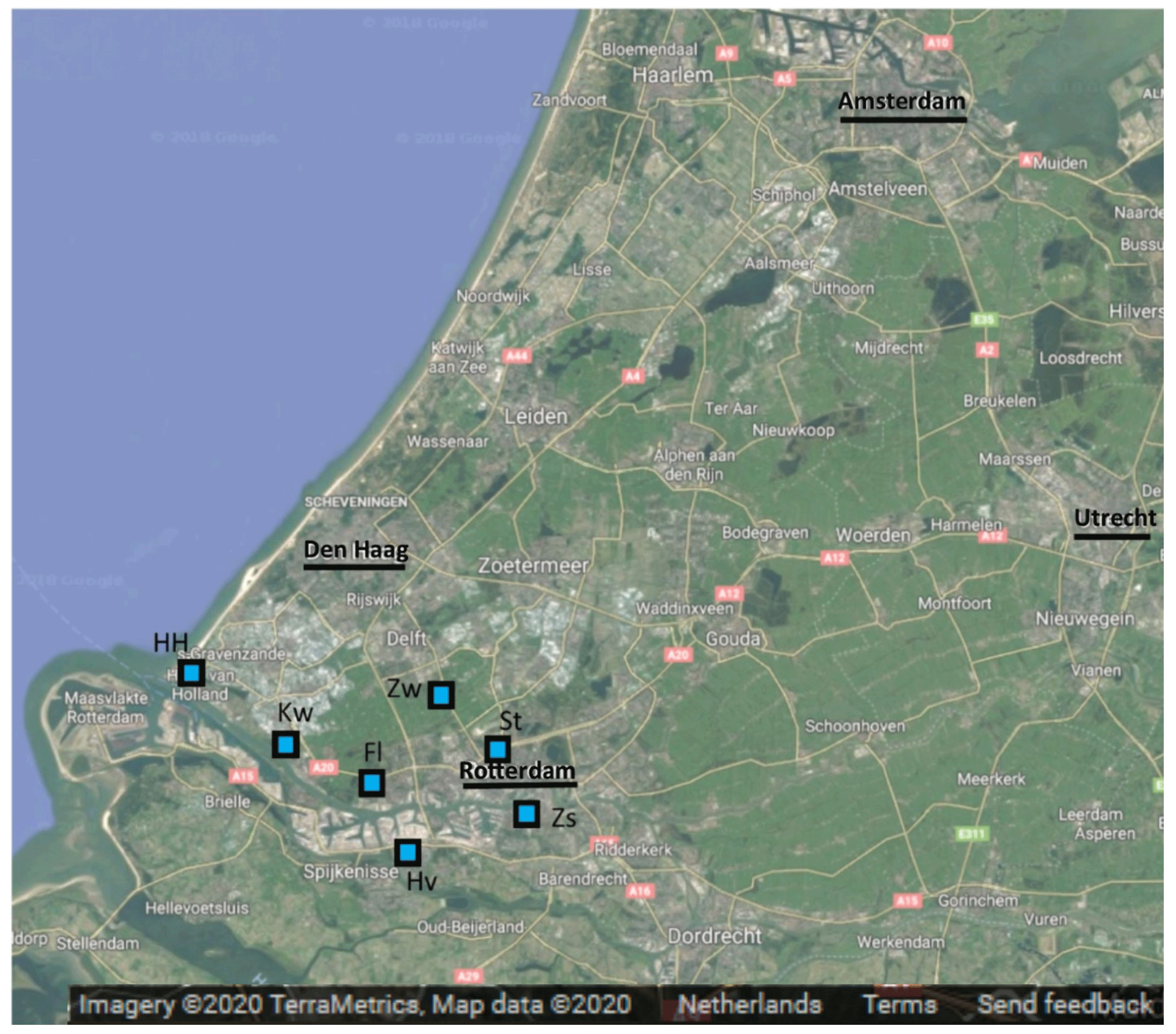
Figure 1Map of the domain covered (Randstad area, the Netherlands) within this study, including major cities Amsterdam, Rotterdam, The Hague, and Utrecht (underlined). The squares show the locations of the measurement sites within the urban network configuration. The area of this domain is approximately 77 km×88 km. Source: © Google Maps.
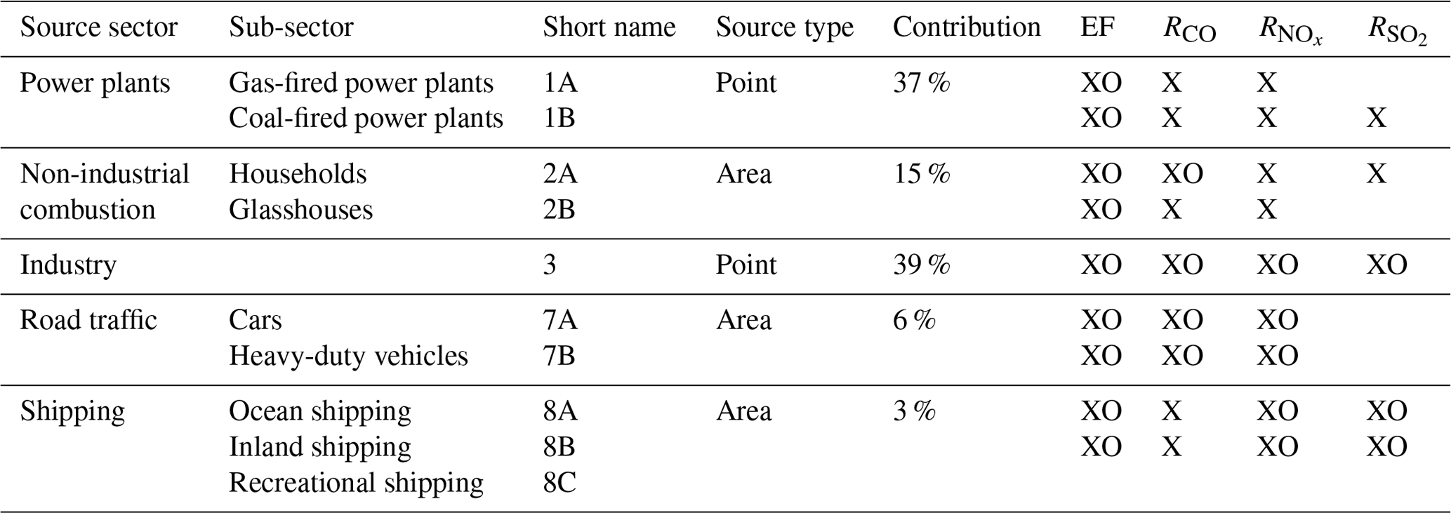
Table 1Overview of source sectors and sub-sectors distinguished in the dynamic emission model, including their short name used in the figures, their source type, and their approximate contribution to the total CO2 emission in Rotterdam (Netherlands PRTR, 2014). Crosses (X) indicate which emission factors (EFs) and tracer ratios of CO, NOx, or SO2 (RCO, , ) are part of the state vector, and circles (O) indicate whether they are also part of the short state vector (see Sect. 2.3).
The ultimate goal is to develop an emission model that assimilates high-resolution activity data, such as near-real-time traffic data. A truly dynamic emission model is not dependent on precalculated annual emissions and spatial or temporal downscaling but directly uses activity data to calculate emissions for that specific moment. However, the development of a dynamic emission model still requires a lot of research. Here, we make a first step by mainly illustrating the potential of using high-resolution activity data to better represent temporal variations.
In this work, the emissions are calculated in four steps. First, the annual national emission is calculated per sector using reported annual activity data and CO2 emission factors. Second, we apply temporal disaggregation to hourly emissions using time profiles based on a combination of default temporal profiles and environmental conditions. Third, we downscale the national totals to 1 km×1 km resolution using statistical data, such as population density. Finally, our approach also allows uncertainties to be described in detail based on parameters in Eq. (2).
2.1.1 Step 1: sectorial total emission calculations
Total annual emissions (FX in kg yr−1) per sector and species (X=CO2, CO, NOx, SO2) are calculated as a function of the economic activity and an emission factor (adapted from Raupach et al., 2007):
where A is the amount of activity (which is often given in EUR when GDP or industrial productivity is used as proxy) and E is the primary energy consumption (petajoule, PJ). RX is the emission ratio needed to calculate emissions of co-emitted species X from the CO2 emissions (kg kg−1), which is specific for each economic sector ( is always 1, others are illustrated in Fig. 2). In this equation the term is the CO2 emission factor (EF), i.e. the amount of CO2 emitted per amount of energy consumed. The term E∕A can be seen as a measure of energy efficiency, in which technological development plays an important role (Nakicenovic et al., 2000).
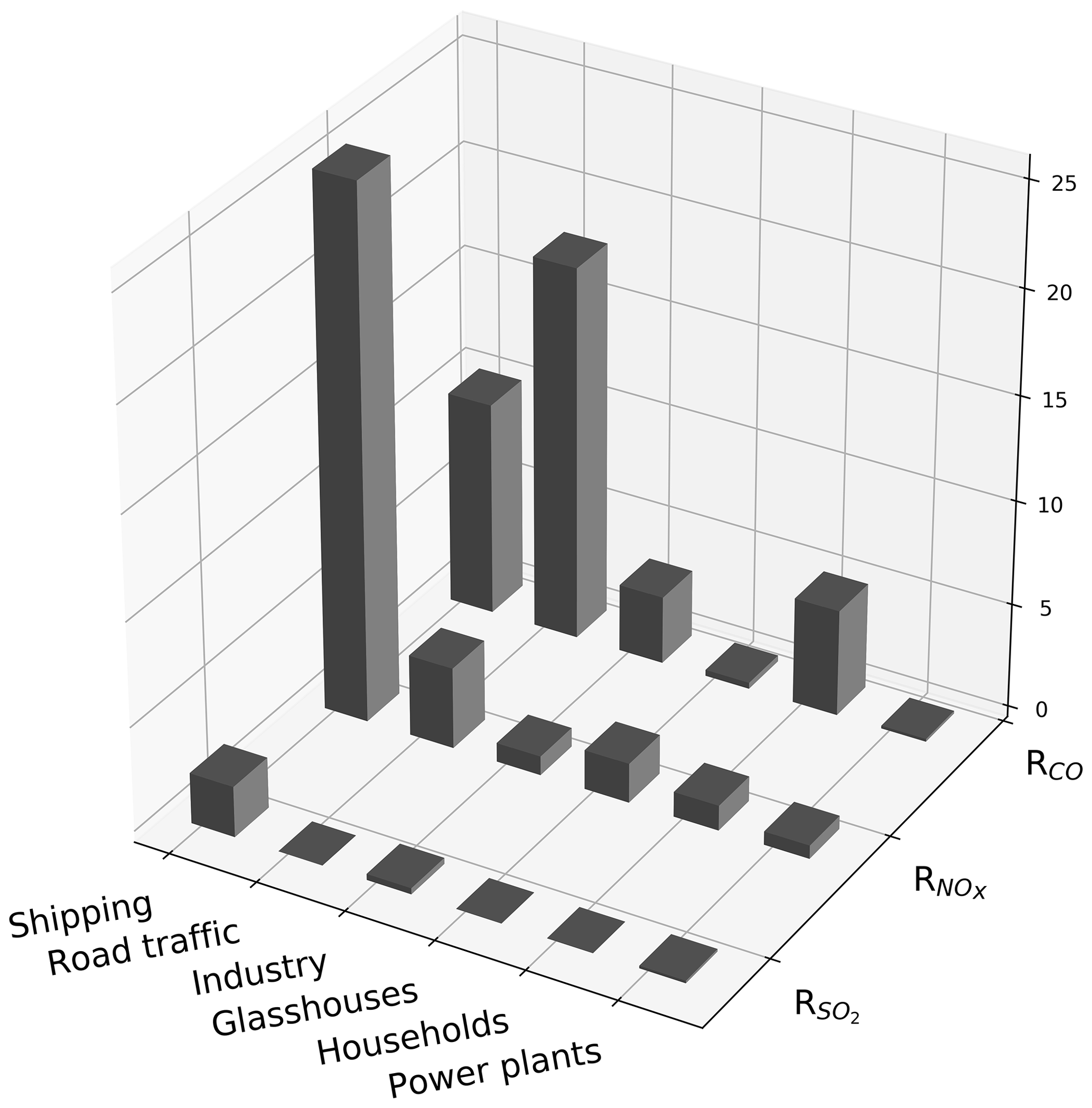
Figure 2Emission ratios of CO∕CO2 (RCO), NOx∕CO2 (), and SO2∕CO2 () for specific source sectors based on the Dutch Pollution Release and Transfer Register (Netherlands PRTR, 2014). Units are in parts per billion per parts per million (ppb ppm−1). A value of 10 on the y axis thus implies that for each 1000 mol of CO2 10 mol of the auxiliary tracer is emitted.
The information needed in Eq. (1) comes from various inventories and national information sources. For example, changes in annual activity can be approximated based on national statistics such as the GDP (gross domestic product), which can be a proxy for industrial activity. Or A can be based on environmental data such as the annual degree day sum based on the outside temperature, as proxy for the need for household heating in a particular year. These proxies for A are known globally, which is why we use Eq. (1) instead of directly using energy consumption data (E). For local studies, more specific activity data could be used, e.g. vehicle kilometres driven as a predictor for road traffic emissions. The second term in Eq. (1) (E∕A, the energy efficiency) can be estimated from activity data and energy consumption statistics, such as those available from the International Energy Agency or data from national statistics agencies. Even if E is not directly available for a country, an estimate can be made based on a country with a comparable level of development and climatology. Note that this term can show a large trend in the case of technological development. The last terms in Eq. (1) (F∕E and RX, the emission factors) are the most uncertain ones, because the emission factor is dependent on the fuel mix and the energy efficiency, which itself can vary with environmental conditions (e.g. a cold engine on a winter day burns less efficiently). It can therefore differ significantly between countries. Emission factor values that are generally valid can be gathered from the Intergovernmental Panel on Climate Change (IPCC) or the European Environmental Agency (EEA), while country-specific values are typically less easily accessible. For our study area, we have access to both EEA data and to Netherlands-specific numbers, as well as Rijnmond-specific values (Netherlands PRTR, 2014). See Appendix A for a full overview of the data used.
2.1.2 Step 2: temporal profiles and parameterizing activity
The second step is to disaggregate the annual emissions to hourly emissions by calculating time profiles, such that Eq. (1) becomes “dynamic”:
where Tt is the hourly time factor and F is in kilograms per year (kg yr−1). Averaged over a year the value of Tt is 1.0, so that it only alters the temporal evolution and not the total emissions. Energy use is often specifically linked to an activity (A in Eq. 1) and Eq. (2) on which temporal information is more readily available than on the resulting emissions. Therefore, Tt can be calculated in two ways: (1) by directly using temporally explicit activity data or (2) by parameterizing temporal variations from environmental and/or economic conditions. When activity data are available, the first option is preferable. However, in data-sparse regions the second option might be necessary to implement, which is still an improvement compared to long-term average profiles as commonly used as we will discuss next for several sectors represented in our emission model. Appendix B provides an overview of the data that are used per sector.
Non-industrial combustion is dominated by household natural gas consumption to heat houses, for cooking, and for warm water supply. A Dutch energy provider has a dataset publicly available from about 80 smart meters for the year 2013 with hourly gas consumption (Liander, 2018). It clearly shows a seasonal cycle but also more small-term variations (daily data are shown in Fig. 3). We also see higher gas consumption in the beginning of the year, when the first 3 months of 2013 had some long, cold spells.
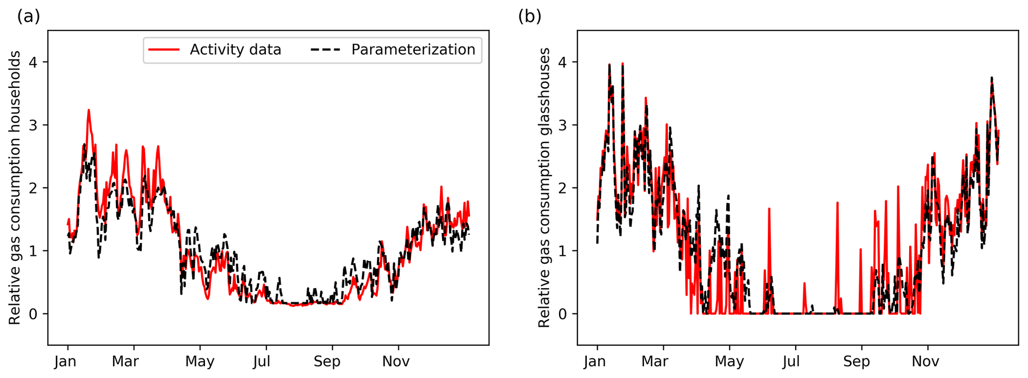
Figure 3Daily time profiles for households (a) and glasshouses (b). Solid red lines are based on true activity data, whereas dashed black lines are parameterizations based on the degree day function.
The use of energy for household heating is connected to the outside temperature. Previous studies have therefore used the concept of heating degree days to describe the temporal variability in emissions from households (Mues et al., 2014; Terrenoire et al., 2015). This method weighs all daily mean temperatures below a certain temperature threshold (here 18 ∘C, as suggested by Mues et al., 2014) and assigns emissions to these days accordingly. Besides heating, gas consumption is related to warm water supply and cooking, which is largely independent of the outside temperature. Therefore, a constant offset is assumed of 20 %, similar to Mues et al. (2014). More details can be found in Appendix B.
We compared the heating degree day method using observed temperature data from the Royal Netherlands Meteorological Institute (KNMI) with gas consumption data on a daily basis (Fig. 3). The degree day function follows the gas consumption data very well, including the higher consumption at the start of the year, reaching an R2 of 0.90 (N=365). The gas consumption of consumers also has a diurnal pattern with peaks in the early morning and late afternoon. Therefore, a diurnal profile can be estimated based on typical working hours, for which we used profiles from Denier van der Gon et al. (2011). For hourly data, R2 is 0.80 (N=8760, not shown).
For the energy consumption of glasshouses, there is no true activity data available. Instead, we use modelled daily energy consumption for a typical Dutch glasshouse cultivating tomatoes (courtesy of Bas Knoll, TNO) as the “truth” (activity data). This time profile is calculated for typical meteorological conditions, such that the order of magnitude and the peaks are representative for an average year. There is almost no energy consumption during the summer, which indicates that there is no constant offset. So, we use the heating degree day function with no constant offset to determine the time factors. Moreover, we use a lower temperature threshold of 15 ∘C to get a better fit with the observed energy consumption. During summer several days show a peak in the relative gas consumption, suggesting that the average temperature has dropped below the threshold. The estimated function compares well with the activity data (Fig. 3) with an R2 of 0.85 (N=365). The diurnal cycle of glasshouse emissions is likely to be different from that of household emissions. Yet we lack data to establish a diurnal cycle. We therefore use the same diurnal profile as for households, although this is likely to be incorrect.
Power plants can use different fuels such as hard coal, natural gas, or biomass. In the Netherlands coal-fired and gas-fired power plants account for 80 %–85 % of the total energy production. The remainder comes mainly from wind energy (5 %–6 %) and biomass burning (5 %–6 %). Power generation data are reported by the European Network of Transmission System Operators for Electricity (ENTSO-E), which has detailed data available for the whole of Europe (Hirth et al., 2018). Coal-fired power plants are currently the main source of energy, and their electricity generation is relatively stable compared to other sources. This sector does, however, show a seasonal cycle with less energy production during the summer months. Gas-fired power plants have a larger temporal variability as they are mainly used as back-up for peak hours, depending also on the amount of renewable energy that is available.
We use the degree day function to estimate the time profiles of both coal- and gas-fired power plants. Linear regression analysis shows that the coal-fired power generation is correlated with degree days (R2=0.17). In this case we use a large constant offset of 80 % and a threshold of 25 ∘C, which were chosen to best match the actual power generation data. The offset is much larger than for households because there is always a basic energy demand from industry. In contrast, the gas-fired power plants are (negatively) correlated with the wind speed (R2=0.13) and incoming solar radiation (R2=0.10), which may indicate a higher need for gas-fired power generation in the absence of renewable sources. Therefore, we replace the temperature in the degree day function with the multiplication of wind speed (threshold of 10 m s−1) and incoming solar radiation (threshold of 150 J cm−2). A constant offset of 10 % is assumed.
The diurnal cycles for power plants can be based on socio-economic factors. For example, the energy demand peaks early in the morning when people get ready to go to work and at the end of the afternoon when they get home. We find this pattern in the actual power generation data, with coal-fired power plants being less variable during the day than gas-fired power plants. The fixed profile from the European MACC-III emission inventory (Denier van der Gon et al., 2011; Kuenen et al., 2014) matches reasonably well with gas-fired power plant profiles, but it is less applicable for coal-fired power plants (Fig. 4). Overall, the estimated profiles for gas-fired power plants (daily or hourly data) have an R2 of 0.31 or 0.32 (N=366 or 8784) when compared to the activity data. For coal-fired power plants, this R2 is 0.17 or 0.21 (N=366 or 8784).

Figure 4Daily time profiles for gas-fired (a) and coal-fired (b) power plants. Solid red lines are based on true activity data, whereas dashed black lines are parameterizations based on observed temperature (coal) and wind speed and radiation (gas). Average diurnal cycle for gas-fired (c) and coal-fired (d) power plants. Solid red lines are based on true activity data, whereas dashed black lines are fixed profiles from the MACC inventory (Denier van der Gon et al., 2011; Kuenen et al., 2014). Shading gives the 1σ variability of the diurnal cycle based on activity data.
The constant offset of 80 % for coal-fired power plants is mainly caused by the energy demand of the industry and other semi-continuous processes. Taking into account seasonal variations in these processes could improve the timing of coal-fired power plant activities, probably increasing the power generation in winter relative to the summer holiday period. Moreover, the renewable energy supply is probably better modelled when taking into account a larger domain, since the energy supply is not just local. With a better prediction of the amount of renewables, we could improve the timing of the gas-fired power plant emissions, which mostly function as a back-up for renewable energy.
The industrial sector consists of a wide range of activities of which some are semi-continuous and only interrupted by maintenance stops, while others follow working hours. This makes it very difficult to predict the temporal variability, especially for the overall sector. Since the largest CO2 emissions are related to refineries and heavy industry, we will focus on these activities. We find a seasonal cycle in the reported industrial activity, with a small decline during the summer and Christmas holidays. However, the variations are very small (max 1 %). Therefore, we assume constant emissions.
Road transport emissions can vary between different road and vehicle types (Mues et al., 2014), but they are also strongly dependent on environmental, socio-economic, and driving conditions (such as the amount of stops, free-flow versus stagnant conditions, and engine temperature). Traffic count data are often used to create average time profiles for road traffic emissions; although, with traffic counts we are unable to account for environmental and driving conditions. Traffic counts for the Netherlands are made available by the Nationale Databank Wegverkeersgegevens (NDW), and similar data are available in many developed countries. We differentiate between two vehicle types (passenger cars + motorcycles (hereafter referred to as cars) and light-duty + heavy-duty vehicles (hereafter referred to as HDVs)) and three road types (highway, main road, urban road). We selected all available locations for 2014 within or close to Rotterdam that distinguish three to five vehicle lengths and filtered for a minimum data coverage of 75 %. This leaves us with 25 highway, 6 main road, and 13 urban road locations. From these data, we make average time profiles (daily, weekly, and monthly) per road and vehicle type, as is often done to disaggregate road traffic emissions. Note that this method excludes any spatial variations (e.g. highways leading towards the city vs. the beach), except for differentiating between road types.
Generally, HDVs show a larger spread due to the low counts during the weekend (Fig. 5). Car counts on weekdays show morning and evening rush hours, and they go down in between. In contrast, HDV counts peak throughout the day and only go down after the evening rush hour. Moreover, the diurnal cycles are different during the weekend than on weekdays. These patterns can be explained from socio-economic factors. Current time profiles are often based on cars and are unable to correctly represent the temporal variability of HDVs. This also affects the spatial distribution of emissions; therefore, we create average diurnal, weekly, and seasonal profiles separately for cars and HDVs for different road types and considering the day of the week. The comparison of true traffic counts and averaged traffic counts results in R2 values between 0.83 and 0.95 for hourly data for the whole year (N between 2665 and 6471 because of gaps in the traffic count data).
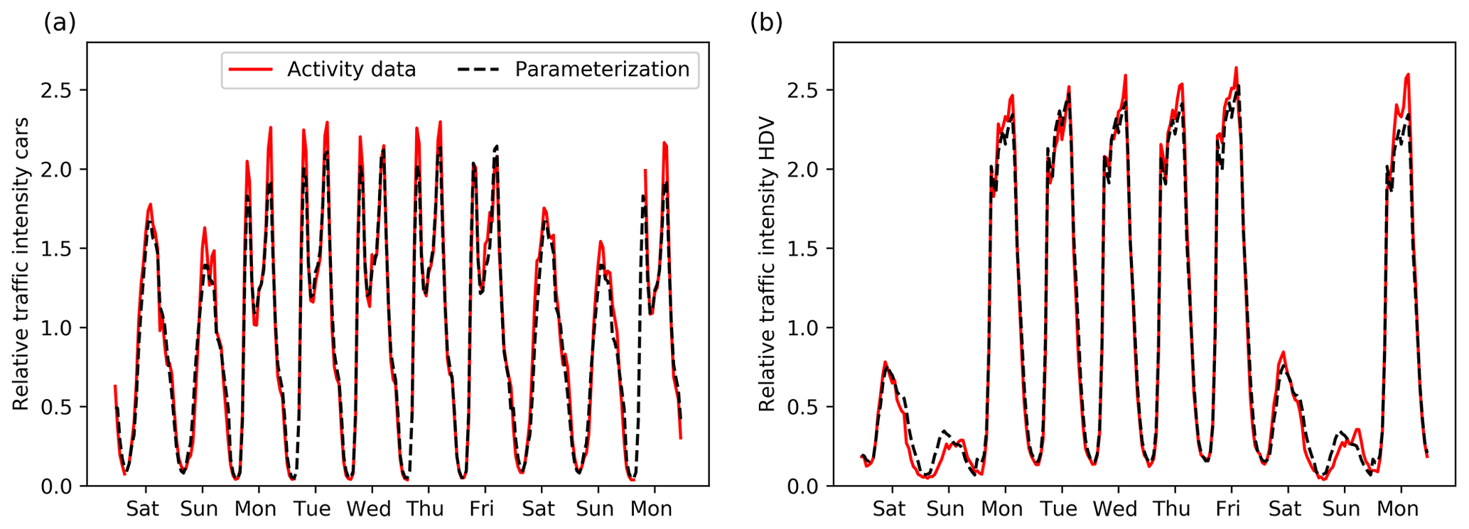
Figure 5Time profiles of passenger cars (a) and heavy-duty vehicles (b) road transport on highways for 10 randomly chosen days in March. Solid red lines are based on true activity data, whereas dashed black lines are parameterizations based on averaged traffic counts for Rotterdam.
Shipping emissions are dependent on the type of fuel used and whether ships apply slow steaming. Additionally, during loading and unloading, ships still emit CO2 and other pollutants, even though they are not moving. Such information is currently not available, so instead we use information about the arrival and departure of ships in the port of Rotterdam to make a time series of ship movements. Note that this only applies to large vessels that transport goods and passengers and that the time profile will look different for recreational shipping. However, large ships account for approximately 80 % of the total shipping emissions in the area of interest. Since we lack information about other types of shipping movements, we will only account for large ships in the time profiles.
We collected ship movements for 1 month (daily data) and an average diurnal profile. The diurnal cycle shows a peak throughout the day, which corresponds well with the HDV road transport emission patterns on highways. The reason for this is that HDV road transport is related to shipping movements, as HDVs take care of part of the goods transported further inland after the goods have arrived by ship. We also find a clear weekly pattern with less ship movements during the weekend, although the decrease is less than for HDV road transport. This is likely because large ships, such as entering the port of Rotterdam, continue travelling during the weekend. Therefore, the weekly pattern resembles more that of car road transport on highways. Thus, we can estimate ship movements by using the temporal profiles of HDVs and cars on highways. This method is specifically tested for Rotterdam and different patterns might be visible elsewhere. We also use HDV patterns for the seasonal variability, and final parameterized and reported activity in this method reach an R2 value of 0.89 for a period of 18 d with hourly data (N=432) as shown in Fig. 6.
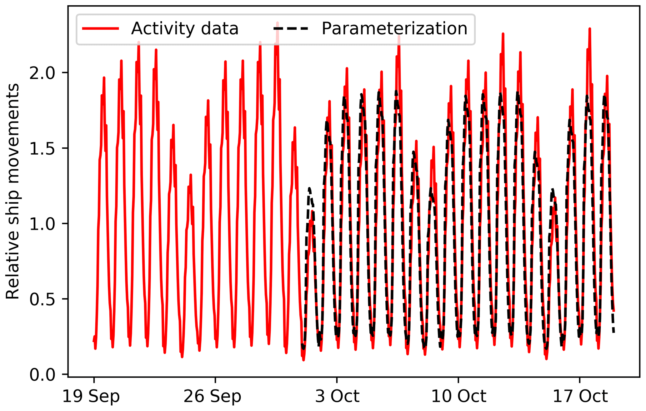
Figure 6Daily time profiles for shipping. Solid red line is based on true activity data, whereas dashed black line is a parameterization based on traffic counts of heavy-duty vehicles (diurnal cycle) and cars (day-to-day variations) on highways.
2.1.3 Step 3: spatial disaggregation
National total sectorial emissions need to be distributed into spatially explicit emissions for our study domain. The spatial disaggregation of emissions has already received attention from inventory builders. Existing emission inventories can be used to describe the spatial disaggregation, if available for the region at high resolution. Therefore, no extra effort is put into the spatial disaggregation, and the spatial patterns from the Dutch Emission Registration have been adopted (Netherlands PRTR, 2014).
In absence of a high-resolution inventory, simple default proxies for the spatial distribution can be used, such as population density (e.g. Gridded Population of the World, GPW) and the presence of roads or waterways (e.g. OpenStreetMap). Generally, these proxies are also used by inventory builders but are often updated to take into account local circumstances. For example, main roads and urban roads are busiest in densely populated areas, and we can assume emissions on main and urban roads are correlated with population density. Highways are used for transport between cities; therefore, emissions take place outside densely populated areas as well. Nevertheless, highway transport is usually to and from densely populated areas, such that most emissions will take place close to cities. We can therefore relate these emissions with the population density in the area of interest (in this case Rijnmond) relative to the rest of the country, which places the same amount of the country-level emissions in our case study domain as the gridded inventory. Additionally, the location of large power plants or industrial plants is often known (for example from E-PRTR, Pollutant Release and Transfer Register), which can be used directly.
Although such information allows us to possibly construct a detailed fossil fuel model in data-sparse regions in the future, in this study we focus first on the more easily implementable and less-developed parameterization of temporal activity in different sectors (step 2) to assess whether this approach is promising enough for future extension.
2.1.4 Step 4: uncertainty analysis
The emission model we have constructed in steps 1–3 contains several parameters per source sector: activity, emission factor, spatial proxy, and time profile. For the analysis, we only consider the emission factors and time profiles, as we assume activity data and the spatial distribution to be (a) well known for our study area and (b) be mostly unobservable from the network of only seven sites which is used here to evaluate our approach (see Sect. 2.2.3). Although the spatial distribution is actually a large source of uncertainty, we aim at optimizing parameter values that are valid for the entire case study area, and for simplicity we ignore the spatially variable uncertainties. Nevertheless, it is possible to incorporate spatial uncertainties in this methodology as well, as illustrated by Super et al. (2020).
As input for step 1 in the dynamic emission model, we use generalized parameters which we take from the IPCC, EEA, and other organizations. These databases also provide an uncertainty range, which we use in a final step to create a covariance matrix. The covariance matrix describes the Gaussian uncertainty of these parameters (diagonal values) and error correlations between parameters (off-diagonal values). From the covariance matrix we create an ensemble of parameters (N=500) that represents their joint distributions, and we use them to calculate an ensemble of emissions. In this Monte Carlo simulation, we transform some Gaussian parameters into log-normal distributions to account for non-negativity or to account for distributions with a very long tail (mainly emission ratios, which can become high in specific cases where no emission reduction measures are taken). Appendix A summarizes the used parameter values and uncertainties (including the shape of the distributions) and shows an example of the covariance matrix. This method is a first step towards a better quantification of parameter uncertainties and error correlations, and additional effort has already been made to improve this method (Super et al., 2020).
In a final step, we select the most important parameters, which are either very uncertain or have a large impact on the total emissions. This leaves us with the 44 parameters that we optimize in a set of data assimilation experiments, described next. In Sect. 3.1 we report uncertainties in per cent (1σ) for normal distributions (CO2) or as a 90 % confidence interval (CI) for log-normal distribution (co-emitted species).
2.2 Data assimilation to estimate fossil fuel sources
The goal of data assimilation is to find a state at which the system is in optimal agreement with observations. In this work, the observations we want to explore are the mole fractions of CO2 and its co-emitted species, while the state of the system is the underlying spatio-temporal distribution of fossil fuel emissions. Such configurations are sometimes referred to as “FFDAS” (fossil fuel data assimilation system) applications, with a number of examples in recent literature (Rayner et al., 2010; Asefi-Najafabady et al., 2014; Basu et al., 2016; Graven et al., 2018). Given the sparsity of approaches explored so far, the dynamic emission model with its parameter-driven emissions we present here could lend itself well for application in an FFDAS, and this is what we explore through a set of experiments with our own data assimilation methodology.
In this study we use the CarbonTracker Data Assimilation Shell (CTDAS) (v1.0) described in detail in van der Laan-Luijkx et al. (2017). Briefly, the CTDAS system is a flexible implementation of a square-root ensemble Kalman filter (Whitaker and Hamill, 2002), which also allows lagged windows (i.e. smoothing instead of filtering). The ensemble Kalman filter optimizes the cost function for unknown variables in the state vector x using information from observations (y0 with covariance R) and a prior estimate of the state vector (xb with covariance P).
In this function, ℋ is the observation operator that returns simulated mole fractions given the state vector. R and P determine how much weight is given to the observations and prior estimate, respectively.
The optimized state vector (indicated with superscript a, whereas b refers to the prior estimates) which minimizes the cost function is
and its covariance is
Here, H is the linearized observation operator, and K is the Kalman gain matrix:
The solutions of Eqs. (4) and (5) are calculated as in Peters et al. (2005) using an ensemble of 80 members. The choice for the ensemble size was based on the typical dimensions of our inverse problem, which has N=1960 observations and M=44 unknowns for the base run.
We have adapted CTDAS for smaller-scale studies by replacing the typical observation operator H, which is the global TM5 transport model (Huijnen et al., 2010), with a combination of WRF-STILT footprints and the OPS (Operational Priority Substances) plume model, building on the methods described in Super et al. (2017a) and He et al. (2018). Moreover, we have added our emission model to the observation operator so that we can sample its parameter distribution in atmospheric mole fraction space. More details about the individual parts of this system are provided below and are summarized in Fig. 7.
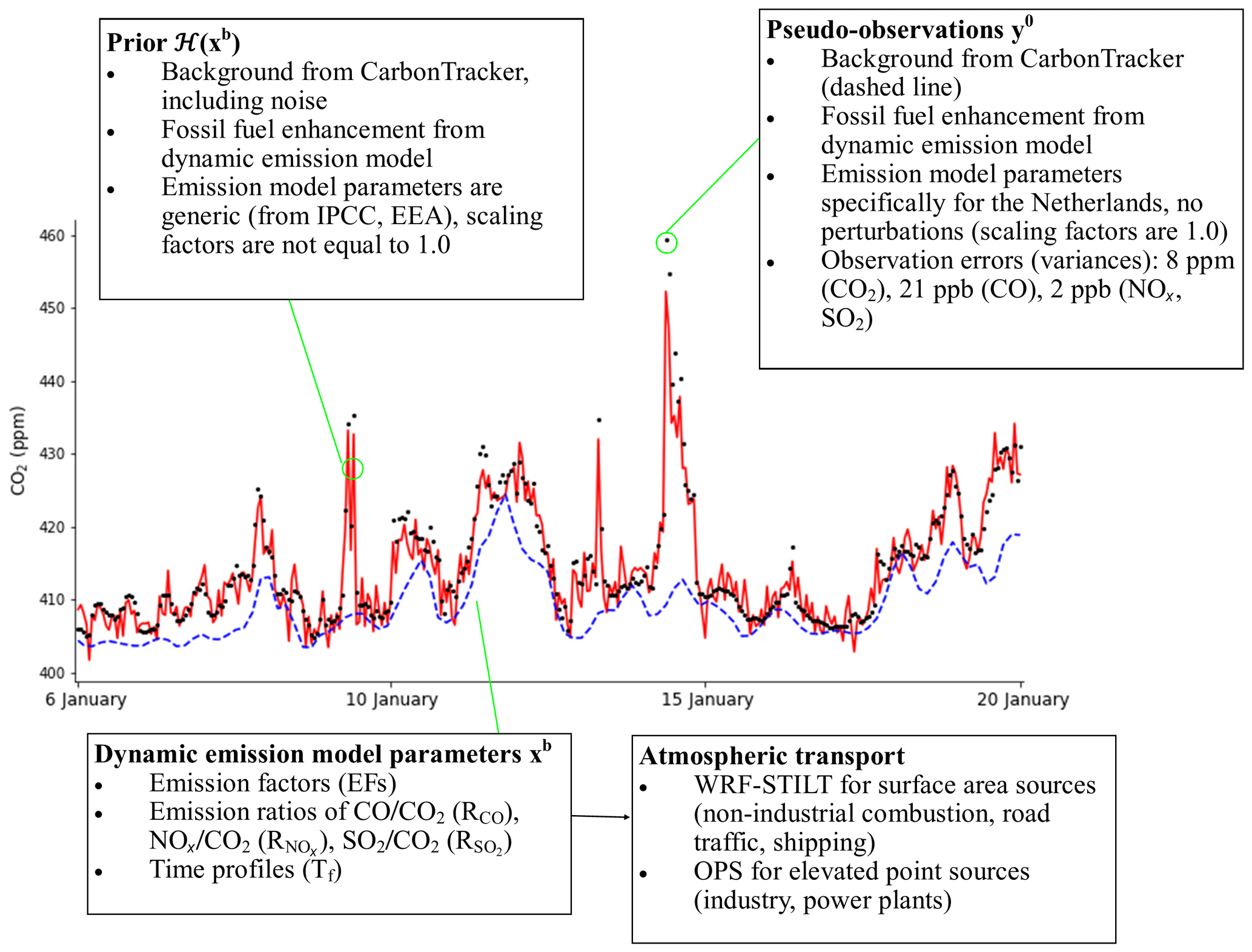
Figure 7Time series of pseudo-observations and prior CO2 mole fractions and a summary of how these time series were created.
2.2.1 Observation operator
The observation operator translates the 44 parameters in the emission model first into emissions (through Eqs. 1 and 2) and then into atmospheric mole fractions. The transport modelling consists of two parts. The first part, the Weather Research and Forecasting-Stochastic Time-Inverted Lagrangian Transport model (WRF-STILT; Nehrkorn et al., 2010) is used for surface emissions that are representative of large areas (i.e. not a point source). STILT is a Lagrangian particle dispersion model that describes the footprint of a single measurement by dispersing particles back in time (Gerbig et al., 2003; Lin et al., 2003). With this footprint the surface influence of emissions on a single observation can be described. An advantage of this method is that it allows for the precalculation of linear atmospheric transport, which makes this part of the observation operator less computationally demanding than running an ensemble of a full atmospheric transport model (like WRF with chemistry). The total domain covered with WRF-STILT is 77 km×88 km (Fig. 1) and includes most of the Randstad.
The second part of the transport modelling is a plume model. In a previous study we have shown that point source (stack) emissions should be modelled with a plume model to better represent the limited dimensions of the stack plume (Super et al., 2017a). Similarly, Vogel et al. (2013) have shown that the surface influence calculated by STILT can lead to large model errors for stack emissions. Therefore, we include the OPS (Operational Priority Substances, short-term version) plume model in our framework to model the transport and dispersion of stack emissions (Van Jaarsveld, 2004; Sauter et al., 2016). OPS provides hourly concentrations at predefined receptor points, which represent our measurement sites. We apply the OPS model only to point source emissions within the Rijnmond area, as we found in a previous study that a plume model only has an added value less than 10–15 km downwind from the stack (Super et al., 2017a). Point sources at more than 10–15 km from the observation site can be sufficiently represented with a Eulerian model. The OPS model input includes detailed information about the exact stack height and heat content of the plume. For more details on WRF-STILT and OPS, see Appendix C.
In addition to the fossil fuel contribution we also include background mole fractions for CO2 and CO. NOx and SO2 are short-lived species; therefore, the variations in the background are relatively small compared to the fossil fuel signals. The CO2 background is taken from the 3-D mole fractions of CarbonTracker Europe (Peters et al., 2010) and also accounts for biogenic fluxes. The resolution of these CO2 fields is , and we select the grid box that is situated over Rotterdam. The 3-hourly data are linearly interpolated to get hourly background mole fractions that are added to the fossil fuel signals calculated by the transport models. We use the strong wintertime correlation between CO2 and CO mole fractions (r=0.73) to calculate CO background conditions from the CO2 background. This is not very accurate, but for the purpose of this OSSE it provides us with a decent estimate of the variability in background mole fractions.
2.2.2 State vector
We populated the state vector with a selection of the most important parameters of the emission model, based on their impact on the total emission uncertainty described in the results (Sect. 3.1). However, we hypothesize that emission model parameters that are not part of the state vector are nevertheless uncertain and may affect the results. Therefore, we include a total of 44 scaling factors in our state vector (xb), and each scaling factor is linearly related to a parameter from the emission model. The uncertainty in these parameters (covariance matrix P) is derived from the Monte Carlo simulations described in Sect. 2.1, with the spread in the emission model parameter values provided by the same databases of the IPCC and EEA. These uncertainty values can also be found in Appendix A.
For this study, we selected an arbitrary 2-week period in January 2014 (6–20 January). Note that during the summer the importance of source sectors might be different, e.g. there will be less heating from households. Nevertheless, this period is sufficient to test the applicability of our DA system. We loop over the 14 d in our study period, resulting in one posterior state vector for each day. We initialize our state vector for every new day using the posterior values and posterior uncertainties from the previous day. Because the footprints we generated extend backwards for 6 h, the state vector for each day is effectively only constrained by the observations from that same day, and hence we did not use a Kalman-smoother approach in this work in contrast to other CTDAS applications.
Although this is a data-rich region, we use generic values for the prior emission model parameters which we take from the IPCC, EEA, and other organizations (Appendix A). These values are typically valid for a large region (e.g. Europe) and not necessarily the best estimate for our regional case study. The reason that we use these values is that they can provide a first estimate of the emissions in data-scarce regions where inverse modelling might add most to our knowledge. With this set-up we can examine how well we can constrain the true emissions starting with this generic, and widely available, information.
One major challenge in this study is to attribute the mismatch between the observed and modelled mole fractions to a specific sector, as a CO2 observation alone provides no details on the origin of the CO2. Therefore, we include three tracers (CO, NOx, and SO2) that are co-emitted with CO2 during fossil fuel combustion in a ratio (referred to as RCO, , and ) that is specific for each source sector (Fig. 2). Their (pseudo-)observations can inform us about the source of the mismatch, but through their emission ratio to CO2 they also constrain the magnitude of CO2 emissions in the emission model. The ratios RCO, , and used for this conversion to CO2 emissions is not fixed: for each of the co-emitted species we included them in the state vector. This recognizes that emission ratios are highly variable and uncertain but play an important role in source attribution.
2.2.3 Pseudo-observations
In this work we create observing system simulation experiments (OSSEs), which use pseudo-observations instead of true observations. The advantage of using pseudo-observations is that we can accurately examine the abilities of our new approach without having to account yet for (often dominant) atmospheric transport errors. This approach represents an ideal situation with relatively few sources of error compared to a study using real observations, which makes it useful to study the potential of this new system to optimize emission model parameters.
The pseudo-observations used to optimize the emission model parameters are created using the same observation operator as described above. The emission model is used to create realistic emissions with a high spatio-temporal resolution. Yet in contrast to the prior state vector, we use specific local (Dutch) values for the emission model parameters. These parameters are considered to be the truth and are therefore not scaled (scaling factors are 1.0). We found that these local parameter values are always within the uncertainty range of the general (prior) values, so that the true solution is part of the distribution explored within the prior state vector. This is confirmed in an experiment with a small model–data mismatch and no noise in the background, which reproduces the true parameters very well (not shown).
The resulting emissions are used in combination with the background mole fractions and transport calculated by WRF-STILT and the OPS model to create pseudo-observations at the locations shown in Fig. 1. For the pseudo-observations, the original background time series are used, whereas in the inversion random noise is added to the background mole fractions with a standard deviation of 2 ppm for CO2. We assume no contribution from biogenic CO2 to the excess CO2 over the background, which means that any biogenic contribution to CO2 within our footprint is the same as in the inflow from outside our domain, which is thus cancelling in the subtraction of the background CO2. An error in biogenic fluxes is therefore attributed to the fossil fuel emissions, which represents a typical case where biogenic and fossil fuel signals are hard to distinguish from each other and from the background. Biogenic fluxes can be significant, even in urban areas, and therefore add significant uncertainty to the fossil fuel flux estimates (Fischer et al., 2017; Sargent et al., 2018).
One simulated time series is illustrated in Fig. 7. The monitoring network consists of seven sites that are scattered over the city of Rotterdam and the port. All sites exist in the national CO2 or air quality measurement networks, although not all species used in the inversion are observed at all locations. We only use the daytime (12:00–16:00 LT, local time) observations to constrain our emissions, resulting in a total of 1960 observations. This is normally done to favour well-mixed conditions when simulated transport is more reliable, and we want to mimic this limitation. We assume all instruments have an inlet at 10m above ground level. In reality this is lower for several sites, but during the well-mixed daytime conditions the difference is minimal. Representing atmospheric transport around in-city sites can be very challenging; therefore, the use of elevated sites or a transport model that can represent transport in complex terrain in more detail is recommended when true observations are used.
The covariance matrix R describes the observation error. It accounts for errors related to instrumentation but also representativeness errors due to model transport, interpolation, and parameterization used in the emission model. Although in principle such errors can be excluded in an OSSE, we prefer to use realistic estimates of these errors to allow for the random errors that we applied to the prescribed boundary inflow, as well as to account for parameters in the emission model that are not optimized even though they contained uncertainty in the pseudo-data creation. We base the R matrix on the calculated errors in the background and atmospheric transport and variability caused by parameters that are not part of the state vector from the uncertainty analysis, and we end up with variances of 2.5 ppm (CO2), 8 ppb (CO), 3 ppb (NOx), and 1 ppb (SO2).
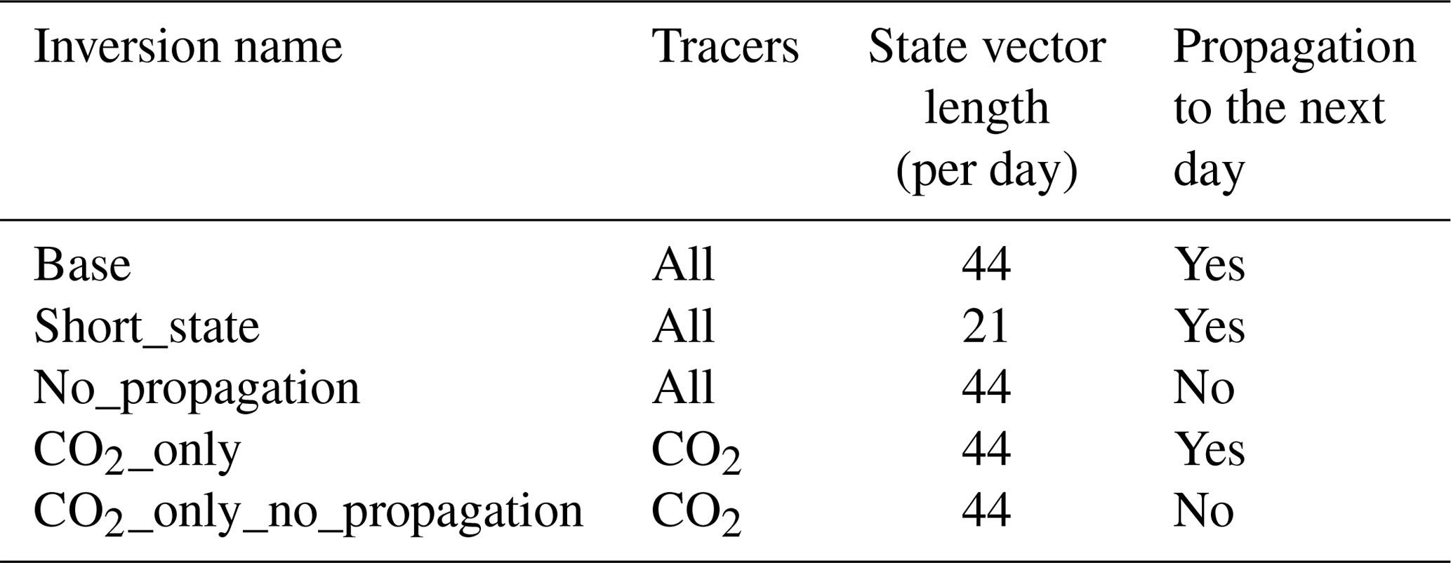
2.3 Data assimilation experiments
We perform various experiments to examine the sensitivity of the system to different set-ups and sources of error. The experiments are discussed here, and the detailed set-up of the inversions is summarized in Table 2. The base run is labelled “Base”.
- 1.
State vector definition. We start with a comparison of two different state vectors. For this purpose, we compare the base run with an inversion (Short_state), which only includes the 21 most important parameters as identified in the sensitivity analysis. This test allows us to examine the impact of erroneous non-optimized emission model parameters on the emission estimates. The results are discussed in Sect. 3.2.
- 2.
Source attribution. Next we compare two monitoring network configurations which differ in the number of tracers used. We perform an inversion with CO2 as the only tracer (CO2_only) and one with the full range of tracers (Base) to assess the added value of including co-emitted species for source attribution. These tests address the question of whether co-emitted species can be used for source attribution. The results are discussed in Sect. 3.2.
- 3.
Propagation. The third experiment is used to examine the effect of propagation of posterior values and uncertainties on the final emission estimates. We compare the base run to a run that has no propagation (No_propagation and CO2_only_no_propagation) but instead starts from the same prior mean and uncertainty on each of our 14 d considered. The runs without would allow the parameter values to change over time. The results are discussed in Sect. 3.3.
Table 2Overview of the inversions: which tracers are included, the length of the state vector, and whether posterior values and uncertainties are propagated.
Before demonstrating the use of our dynamic emission model in an inverse framework, we demonstrate its application as a simple but versatile method to generate hourly gridded emissions for multiple species with full covariances.
3.1 Dynamic emissions and their uncertainty
The total annual emission of CO2 for the Netherlands calculated with the dynamic emission model is 180 Tg CO2 with an uncertainty of 15 % (1σ Gaussian based on 500 members of a Monte Carlo simulation). This matches the total of the Dutch national emission inventory for 2014 by design (step 1), but the uncertainty on the latter was estimated with a similar Monte Carlo simulation to be only 1 % for CO2 in 2004 (Ramírez et al., 2006). This smaller uncertainty is fully due to the use of country-specific emission factors with a much smaller range than we derived from the IEA and IPCC inventories. Spatial disaggregation (step 2) does not affect the uncertainty of the domain-aggregated annual fluxes, and the time profiles (step 3) have no impact on the annual total emissions. For CO, NOx, and SO2, the uncertainties in the emission model are much larger, with medians (CIs) of 6.5×10⁸ (1.3×10⁸–6.8×10⁹) kg CO yr−1, 5.0×10⁸ (1.2×10⁸–5.1×10⁹) kg NOx yr−1, and 1.3×10⁸ (5.1×10⁶–2.2×10¹⁰) kg SO2 yr−1. These ranges result from uncertainties in the assumed ratios of their release per unit of CO2 emitted.
At the sub-annual timescale, time profiles have an impact on the uncertainties as well. The daily emissions of the Netherlands depend on the day and the season (Fig. 8) and range from 0.36 to 0.76 Tg CO2 d−1. The time series shows a seasonal cycle with lower emissions during the summer. There is a clear weekly cycle with reduced emissions during the weekend. The uncertainty in the total daily emission varies between 8 % and 15 %, which is similar to or lower than the uncertainty in the annual total emissions. The explanation for these relatively low uncertainties is that many uncertainties are temporally uncorrelated, and their impacts on individual days partially cancel out. Moreover, the largest sectors (coal-fired power plants and industry) already have a large uncertainty and adding more uncertainty through the time profiles has little impact. Nevertheless, the uncertainties introduced through the time profiles cause an uncertainty in daily CO2 emissions of about 7 % if the other uncertainties are excluded from the analyses.
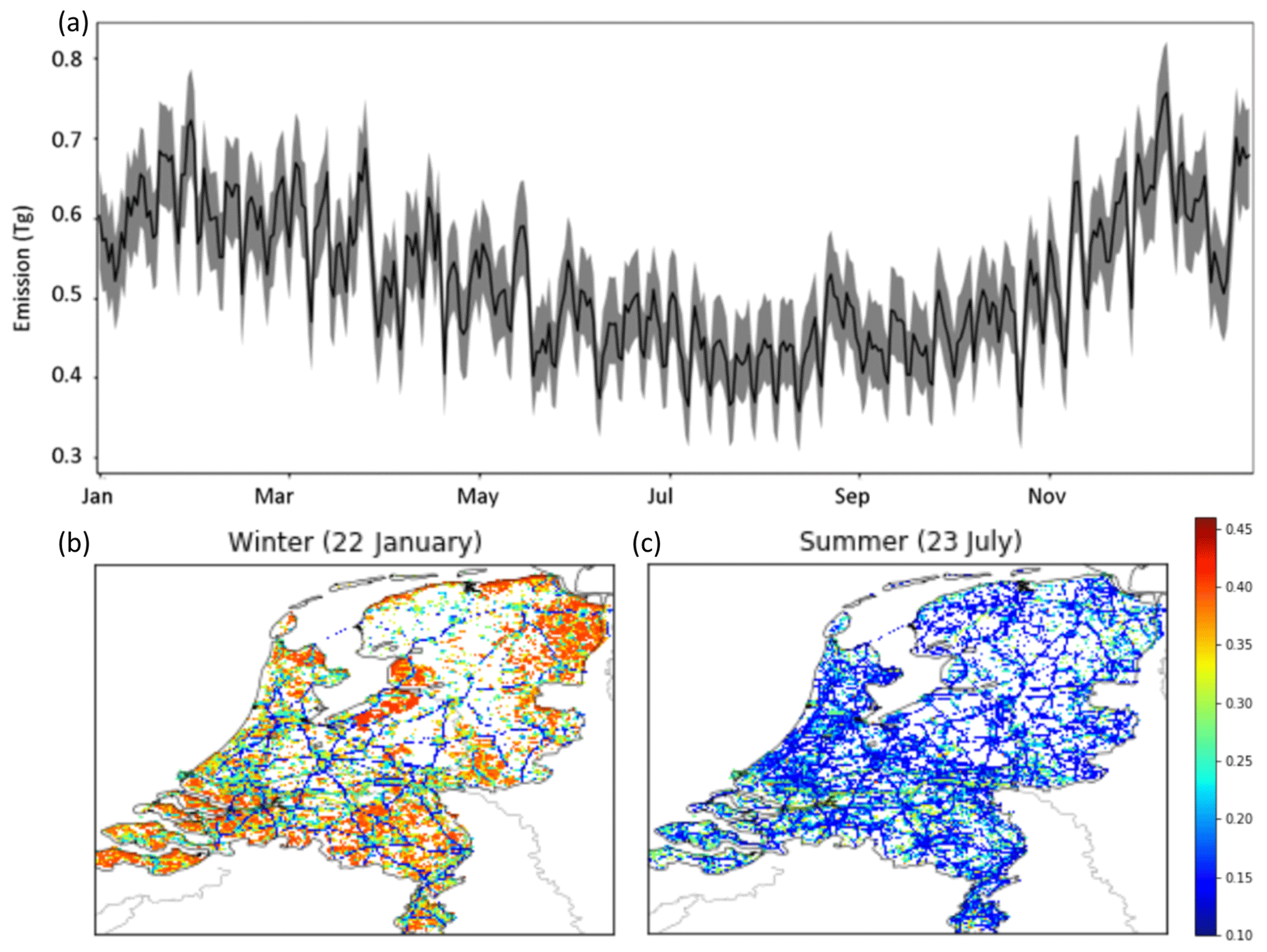
Figure 8(a) Time series of daily CO2 emissions (in Tg CO2 d−1) and their uncertainty. Given is the interquartile range (shaded area) and the median (line) from the ensemble. (b, c) Map of annual mean relative uncertainty of emissions for the top 25 % of pixels with the largest emissions, during a winter month (dominated by household gas and electricity use) and a summer month (electricity and road traffic dominated).
Differences in the relative contribution of different sectors are evident when looking at the map of uncertainties across the Netherlands (Fig. 8), reflecting both the most uncertain parameters but also the dominant source sectors. Winter emissions, for example, are dominated by household gas usage, while industrial and traffic emissions give rise to uncertainty all-year round at a 10 %–30 % level. We further identified the most important parameters per source sector with a Monte Carlo simulation per source sector (Fig. 9). Results show that the road traffic and shipping sectors contain the smallest relative uncertainties, although the time profile for shipping causes an uncertainty of about 7 % in the total shipping emissions. The industrial emissions are most uncertain, and this is almost exclusively due to the emission factor, which causes an uncertainty of 41 % in the total industrial emissions. Similarly, the power plant emissions have a large relative uncertainty due to the uncertain emission factor of coal-fired power plants (19 %). Also, for households and glasshouses, the emission factor is uncertain (14 % and 26 %, respectively), but here the time profiles also have a large impact (10 % and 16 %, respectively).

Figure 9Box plots showing the uncertainty in the CO2 emissions from power plants (1A + 1B), households (2A), glasshouses (2B), industry (3), road traffic (7A + 7B), and shipping (8A + 8B + 8C) caused by individual parameters affecting that sector. Uncertainty is represented as the spread in daily (normalized) emissions from each ensemble member (N=500) for a randomly chosen day. EF refers to an emission factor (green bars) and T to a time profile (orange bars). (Sub)sectors are indicated with their short names as summarized in Table 1. Note that the time profiles of road traffic emissions are specified per road type (1 = highway, 2 = main road, 3 = urban road). Minor parameters that have very small impacts on CO2 emissions are not shown here (23 out of 44).
3.2 Optimizing dynamic emissions
In the base inverse modelling set-up, our system is able to improve the mean estimate and reduce the uncertainty on total CO2, CO, NOx, and SO2 emissions. Figure 10 shows the probability density function of these estimated total emissions, compared to the prior (using parameters derived from IPCC/EEA) and the truth (created with country-specific parameter values). Interestingly, the posterior result deteriorates slightly when using a shortened state vector in which 11 parameters of “minor” influence (such as the SO2∕CO2 ratio of household emissions) are not optimized from their incorrect prior. This is caused by sporadic atmospheric signals that are dominated by household emissions, even if these emissions only contribute a small fraction to the total emissions. These signals are then used to update the emission factor, while the emission ratios are also incorrect.
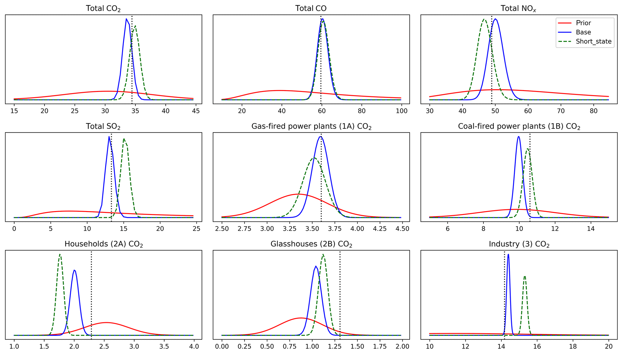
Figure 10Probability density functions of emissions per species or per source category (for CO2) in units of teragrams (Tg) (CO2) or gigagrams (Gg) (CO, NOx, SO2). The truth is shown as a vertical dotted line, typically well matched by the mean of the posterior in blue. Using a shortened state vector (green dashed line) deteriorates the total non-CO2 emissions substantially and leads to misattribution of CO2 emissions in minor categories such as 2A (households).
With CO2 as the only tracer in the inversion we find that we can still estimate total CO2 emissions (truth minus optimized equals 0.03 Tg CO2 yr−1), but we lose the capacity to attribute emissions to specific sectors. Instead, mainly the emission factor of the largest single source, being industry (EF3), is optimized. We illustrate this in Fig. 11 using the No_propagation run. The large spread across the 14 individual days indicates that the emission factor jumps around within a large prior uncertainty distribution and is not well constrained on each day. Some of the other emission factors show almost no deviation from the prior and little variability. Given the constraints posed by CO2 observations alone, and the limited number of parameters that change the simulated CO2, optimizing EF3 improves the results at the lowest costs. Introducing the co-emitted species allows the system to identify the source of a residual and attribute it to the right parameters if sufficient sensitivity is present. This is especially true for those sectors that have relatively small emissions and/or uncertainties (like 2B and 1A). This is corroborated by the posterior covariance matrices (see Appendix D) which show a reduction in parameter correlations for those parameters (i.e. a better mathematical separation of the estimates) when all tracers are included in the estimate. For other parameters, the median values are further from the truth than the prior (e.g. for 8), which indicates that there is too little sensitivity to these parameters.
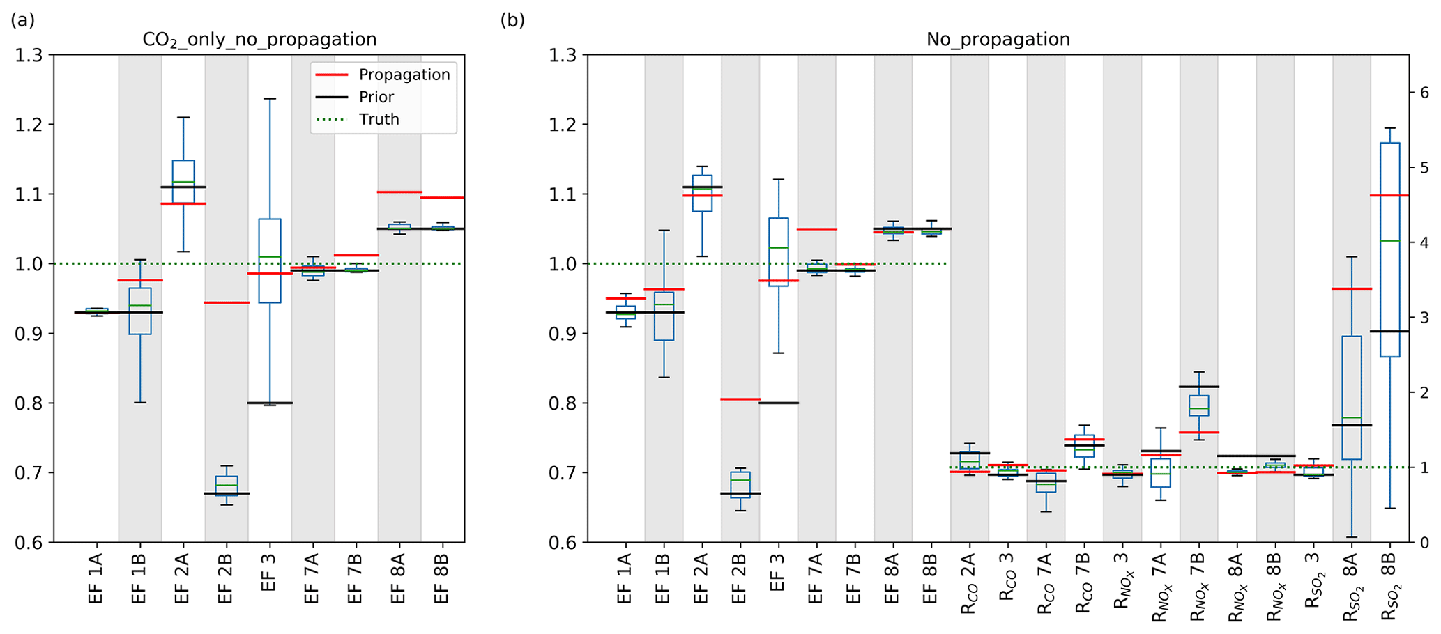
Figure 11Spread (Q1–Q3) and median values of the parameter scaling factors for the 14 individual days included in the CO2_only_no_propagation (a) and No_propagation (b) inversions and final value of the CO2_only (a) and base (b) inversion (red lines). The prior values are indicated by the black lines and the truth is indicated with the green dotted lines (value of 1.0). The left y axis is for the emission factors and the right y axis for the tracer ratios. The inversion with all tracers shows more variability in the emission factors and larger deviations from the prior values.
3.3 Localization and propagation of information
Propagating information on parameter values from one day to the next is often better than using the median of an individual day's estimates as illustrated by the red lines in Fig. 11. Nevertheless, the sporadic detection of plumes with specific signatures suggests that a form of selection or localization of the strongest signals could reduce noise and improve the estimate for the No_propagation run. We therefore ranked the 14 daily independent parameter estimates based on their relative posterior uncertainty and the residuals in an attempt to find the most trustworthy parameter values. This ranking is done per parameter, so the best estimate of different parameters can be related to different days. The increase in residual (same for all parameters) and posterior uncertainty (of the industrial emission factor) is shown in Fig. 12, where the three to five highest-ranked days have similar characteristics after which the reliability decreases. On the lower-ranked days, atmospheric signals from that particular source sector are too small (or even absent) to update the parameters related to that source sector. A similar pattern is found for the other parameters (not shown), with 2–5 d of high sensitivity out of 14.

Figure 12Increase in posterior uncertainty (1σ of unitless scaling factor) in the industrial emission factor (EF 3) and absolute mean residual of CO2 (in ppm) from highest- to lowest-ranked days.
When we use the top-three averaged parameter values to calculate emissions, we find for most sectors that the emission estimate is similar to the base run, albeit with a larger uncertainty, while for a few specific sectors results deteriorate. This suggests that selecting for strong signals can dampen spurious noise but still does not improve on the base run that includes full propagation of the covariances and hence carrying information on parameter correlations that is partially lost in the No_propagation run.
From the posterior covariance matrices we can confirm our selection of “good” days, as these typically show relatively weak correlations between parameters. For the industrial sector (emission factor, , ), these are typically weak on most days, and indeed the mean over the entire period already gives a robust estimate of the true parameter value (Fig. 13). The parameters with the strongest correlations are RCO of households and road traffic, and their mean values tend to be dominated by a few outliers. Selecting days on which the posterior parameter correlations are weak (i.e. the atmospheric signal clearly contains information about this specific parameter) results in a large improvement compared to the prior or a 14 d average. Moreover, these results show a similar or better performance as the top-three selection based on Fig. 12 (0.08 for EF3 and 0.18 for RCO 7A, not shown), and are closer to the base run.
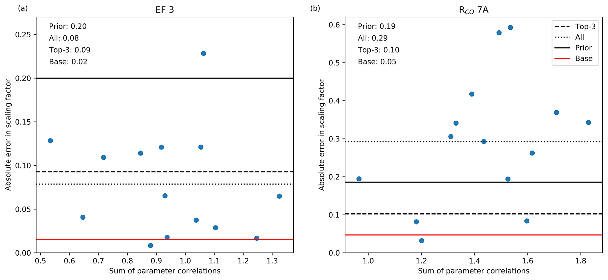
Figure 13Scatter plot of the absolute error in the scaling factor of the industrial emission factor (EF 3) and RCO of road traffic (7A) against the sum of the parameter correlations of the same parameters. The correlation coefficients are −0.17 and 0.37, respectively. The horizontal lines give the average absolute error in the scaling factor for the prior (full black line), if all 14 d are averaged (dotted line), and based on the 3 d with the smallest parameter correlations (dashed line) and the result for the base run (full red line). The values are also given.
4.1 Optimizing the dynamic emission model
The dynamic emission model has the advantage over static emission fields that its parameters are optimized, giving more detailed physical meaning to the results. To reduce the size of the problem, the state vector can be populated with those parameters that are most important and/or uncertain. However, we find that other uncertain parameters that are not part of the state vector can still significantly affect the optimization. Therefore, the size of the state vector should be considered carefully when applying this method. How to best determine the size of the state vector requires further work, possibly using some objective criterion to select for a dynamic model with an optimal information content (Akaike, 1974). Moreover, we performed an experiment to establish the possibility to optimize the time profiles as part of the state vector. Although we found small improvements for some sectors, it appears to be difficult to differentiate between the different variables in Eq. (2) that have a linear relationship based purely on the observations. Therefore, the results are not shown and optimizing the temporal dynamics of the emission model requires further work. In a future study the uncertainty caused by spatial disaggregation should also be included, as well as the possibility to reduce this uncertainty using higher-resolution satellite observations (Kuhlmann et al., 2019).
Additionally, we identified the base run as the simplest method to get good estimates, but we do note that our current propagation scheme does not yet include error growth. That means that eventually the ensemble will converge on a parameter value and discard incoming observational evidence unless the covariance is inflated to allow new updates. Examples of such a covariance inflation scheme are ample in literature and in principle not difficult to include but were not yet considered in this work as the time periods covered were still short. An example related to this work is to use weather system characteristics to determine a correlation length for household emissions.
Finally, we have demonstrated that tracers are suitable for source attribution. Several previous studies have used co-emitted species as tracer for fossil fuel CO2 by taking advantage of the specific emission ratio characteristics of each source sector (Lauvaux et al., 2013; Lindenmaier et al., 2014; Turnbull et al., 2015) and came to similar conclusions. Nevertheless, the uncertainty in emission ratios remains a source of error; therefore, the optimization of emission ratios with our system is a promising step forward. Using co-emitted species to identify the total fossil fuel contribution to the observed CO2 signal is more difficult (Turnbull et al., 2006). The reason for this is that there is a large variability in emission ratios between sectors. This makes it difficult to establish an average emission ratio for an urban area, because it depends strongly on the relative contribution of each source sector and may vary over time.
4.2 Radiocarbon and background definition
Therefore, a nice addition to this inversion system would be the inclusion of radiocarbon measurements. The radiocarbon isotope (14CO2) can be used to simulate fossil fuel CO2 records and has been applied successfully in several inverse modelling studies (Turnbull et al., 2006, 2015; Levin and Karstens, 2007; Miller et al., 2012; Basu et al., 2016; Wang et al., 2018). The radiocarbon measurements could be used directly in the inversion (as we did with the co-emitted species) or be used to define a fossil fuel CO2 record in advance (Fischer et al., 2017; Graven et al., 2018). Our urban network detects average fossil fuel CO2 signals of about 5 ppm with peaks up to 50 ppm. This would result in Δ14C signals (the ratio of 14CO2 to 12CO2) of around 13 ‰ up to 130 ‰, which are certainly detectable with current techniques. However, observations of carbon isotopes are expensive and currently not widely available, so their applicability is still limited. Besides Δ14C, other isotope signatures and tracers can also provide additional information. For example, 13CO2 and O2∕N2 can give insight into the dominant sources and sinks or fuel types (Lopez et al., 2013; Van der Laan et al., 2014) and as such be an indicator for the transition from fossil fuels to biofuels. They might also help to separate between the stack emissions of industry and coal- and gas-fired power plants.
An additional advantage of including the radiocarbon isotope is that the uncertainty in the background CO2 can be excluded, i.e. only the fossil fuel record is considered. Here, we choose to ignore the uncertainty in the background, except in the definition of the covariance matrix R, and attribute all tracer residuals to the fossil fuel emissions. Yet an incorrect definition of the background causes a large bias in the optimized emissions (Göckede et al., 2010). There are also several other methods to deal with the non-fossil fuel related CO2 signals. First, the uncertain background can be added to the state vector and be optimized in the inversion. For example, He et al. (2018) have shown that high-altitude aircraft observations are suitable to improve regional biosphere flux estimates by correcting the bias in boundary conditions. Second, a mole fraction gradient over the area of interest can be calculated using an upwind and downwind site such that the boundary inflow plays no role anymore (Turnbull et al., 2015). This method was shown to reduce the impact of boundary inflow but only when the wind direction is more or less perpendicular to the gradient (Bréon et al., 2015; Staufer et al., 2016). Therefore, this method limits the amount of useful measurements.
4.3 Error correlations
The emission model also allows us to study the correlations between model parameters and therefore giving more insight into how information can be used in the system and which parameters are more challenging to separate. Previously, Boschetti et al. (2018) have used the presence of error correlations between emissions of different species and found that this reduces the posterior uncertainties for all species. They even show that the uncertainty reduction increases with the correlation and that an incorrect definition of the error correlations may cause a systematic bias in the posterior emission estimate. However, error correlations are only beneficial if the atmospheric observations can distinguish between the correlated parameters. If this is not the case, the presence of parameter correlations can result in poorly constrained parameters and/or large posterior uncertainties. This is especially true when parameters are sensitive to parameter correlations, as we show for RCO of road traffic.
An important question is then why some emission model parameters are more sensitive to the presence of parameter correlations than others. One hypothesis is that parameters with a lower prior uncertainty are more sensitive to the presence of parameter correlations. The idea behind this is that if we reduce the diagonal value (uncertainty) by a factor of 4, the off-diagonal value (parameter correlation) reduces by a factor of 2. This means that the parameter correlation is relatively stronger if the uncertainty is lower (Boschetti et al., 2018). This hypothesis cannot be confirmed by our results, as we only find a correlation of −0.27 between the prior uncertainty and the sensitivity to parameter correlations (defined as the correlation between the posterior uncertainty and the sum of the parameter correlations). The main difficulty here is that not all parameters can be discerned with the observed atmospheric signals. Although we included the additional co-emitted tracers for source attribution, the emission ratios have a large uncertainty and the system can have difficulties assigning residuals to either the emission ratio or the emission factor. Yet if we calculate an average sensitivity and total posterior uncertainty per sector (by combining the emission factor and emission ratios per sector), we find a correlation coefficient of −0.82. This suggests that this hypothesis might indeed be correct and source sectors with larger parameter uncertainties are less sensitive to the presence of parameter correlations.
4.4 Atmospheric transport model errors
In addition to the experiments described in Sect. 2.3 we conducted an experiment that focused on the role of transport model errors by using observed meteorology to drive the OPS model in the inversion. Like many authors before us (McKain et al., 2012; Brioude et al., 2013; Lauvaux et al., 2013; Bréon et al., 2015; Boon et al., 2016) we found a large impact on the performance of our system and once again confirmed the need for accurate transport models. This experiment is not further shown in this work because of its redundancy with previous conclusions. Nevertheless, we performed this experiment to examine whether transport errors are important when the state vector consists of parameters that are valid for the entire domain. Random errors, such as errors in the wind direction, are unlikely to affect the optimized emissions much when averaged over a longer time period and domain. This was shown by Deng et al. (2017), who found little variation in the average CO2 emission for Indianapolis using different configurations of WRF to calculate the transport. However, they did find an impact on the spatial distribution of the emissions. This becomes important when optimizing a specific source sector that is clustered in one place, such as the glasshouses. We found that the glasshouse sector is only correctly optimized with a specific wind direction. If the modelled wind direction is wrong the residuals would thus not be attributed to the glasshouse sector as it is not in the modelled footprint of the measurement site. As such, we conclude that the footprint definition has an impact on the optimized parameters, despite that the parameters have no spatial distribution. Similarly, Broquet et al. (2018) mention that the location and structure of a simulated urban plume might differ significantly from the true plume characteristics due to errors in the simulated wind speed and wind direction.
Systematic errors, whether in the modelled transport or in the observations, are more difficult to solve as they do not cancel out when simulating a longer period, and this can lead to biased emission estimates (Meirink et al., 2008; Su et al., 2011). Several methods have been suggested to overcome problems with an incorrect description of atmospheric transport, such as using an ensemble of atmospheric transport model simulations (Angevine et al., 2014) or the assimilation of meteorological observations (Lauvaux et al., 2013). The latter showed lower biases in buoyancy and mean horizontal wind speed. Another method that is often used is the selection of well-mixed afternoon hours to exclude stable conditions under which pollutant dispersion is often poorly represented (Lauvaux et al., 2013; Bréon et al., 2015; Boon et al., 2016). Such data selection, however, leads to a bias in the estimated emissions when the diurnal cycle is not correctly accounted for (Super et al., 2020).
Here, we also applied a daytime selection criterion to mimic this situation. However, we found that night-time hours could be very useful to constrain our emissions. In our DA system we use residual fossil fuel enhancements over a background (prior minus true mole fraction enhancement) to constrain the fossil fuel fluxes. The larger the residual, the more information can be gained from it since the impact of the observation error (R matrix) is relatively small. If, for example, the industrial emission factor is underestimated by 10 %, the residual industrial enhancement (given a linear relationship between the emission factor and the total emission from this sector) will be 10 % of the pseudo-observed mole fraction. This means that a large signal from the industry is needed to reach a residual that is larger than the observation error (σ is 1.6 ppm for CO2). Looking at the time series of pseudo-observations we find that such large signals mostly occur during night-time or in the early morning. Therefore, the inversion could benefit strongly from an improved description of night-time boundary layers and stable conditions, so that the large night-time enhancements can be used to constrain the fossil fuel fluxes.
The aim of this study was to examine how well our DA system can quantify urban CO2 emissions per source sector. Since the prior consists of a dynamic fossil fuel emission model, the model parameters are optimized rather than the emissions themselves. The parameters are related to specific source sectors, and to attribute residuals to these sectors measurements of additional tracers (CO, NOx, and SO2) are included in the inversions. We tested this system to examine its ability to overcome some major limitations in current urban-scale inversions: source attribution, definition of the prior and its uncertainties, and the sensitivity to errors in atmospheric transport.
We find that inverse modelling at the urban scale is feasible when the observations contain a lot of information about the different source sectors. Based on this work we can conclude the following:
- 1.
A dynamic fossil fuel emission model can be useful to create a prior in data-sparse regions or to make use of local data to increase the spatio-temporal representation, while allowing us to constrain physically relevant parameters in more detail.
- 2.
When only CO2 mole fractions are used in the inversion, the total CO2 emissions are well constrained, but additional tracers are an important addition to the inversion framework in order to discern the information belonging to specific source sectors and emission model parameters. However, even more tracers might be needed to fully capture the heterogeneity of the emission landscape.
- 3.
The prior error covariance structure based on the emission model provides useful insight into how parameters interact and what is needed to separate them.
Nevertheless, several challenges remain. Transport modelling at this small scale needs to be improved to be able to use real urban observations, as under current conditions the transport error strongly dominates the results. Especially improving the description of night-time boundary layers could be beneficial, because large atmospheric signals mostly occur during this period. For the future, additional advances need to be made to include satellite observations in the inverse modelling framework. The advantage of satellite data is that they cover data-sparse regions and with a larger view they can differentiate between the urban dome with high pollution levels and the cleaner rural areas, which is a nice addition to in situ measurements.
Table A1Overview of all parameters in the dynamic emission model, their unit, function type, expected value, and uncertainty (range).
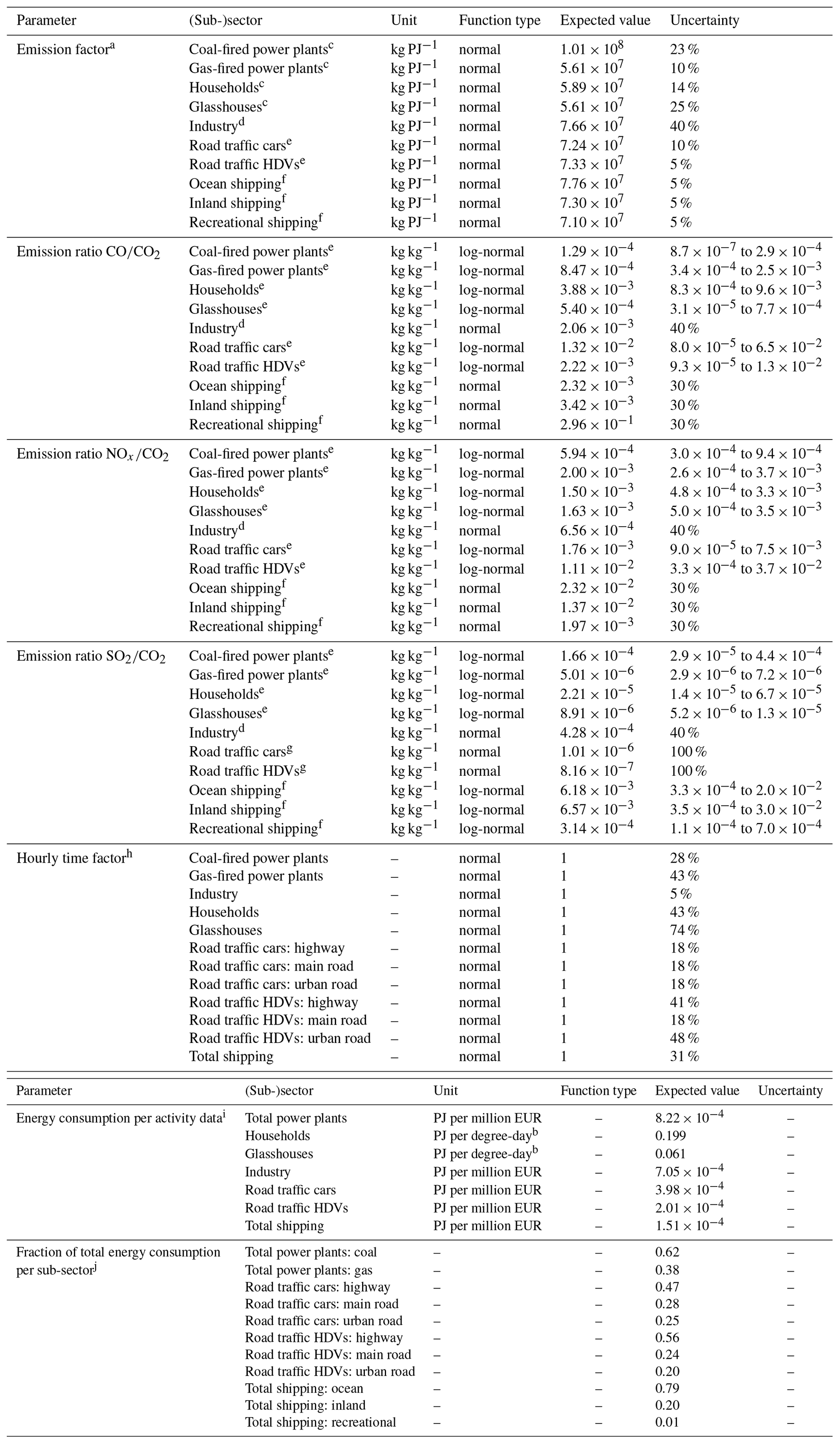
a Emission factor for coal-fired and gas-fired power plants include uncertainty due to variations in fuel type, including burning of biomass (5 % uncertainty). For households, assume 8 % wood combustion based on CO2 emission values (Vernieuwd emissiemodel houtkachels by Jansen (2016); the remainder is natural gas (with 10 % uncertainty). For glasshouses, assume only natural gas combustion, including 20 % additional uncertainty due to use of cogeneration plants. For road traffic cars, assume 69 % gasoline, 29 % diesel, and 2 % LPG (liquefied petroleum gas) (with 5 % uncertainty); for road traffic HDVs, assume 100 % diesel. b using degree day method. c Expected value and uncertainty based on IPCC Emission Factor Database (EFDB) using 2006 IPCC guidelines. d Expected value based on Netherlands PRTR (emission) and Statistics Netherlands (energy consumption); uncertainty based on expert judgement. e Expected value and uncertainty based on the EMEP/EEA air pollutant emission inventory guidebook 2016. f Expected value and uncertainty based on CO2, CH4, and N2O emissions from transportation-water-borne navigation by Jun et al. (2000). g Expected value based on Air Pollutant Emission Factor Library (Finish Environment Institute); uncertainty based on expert judgement. h Uncertainties based on comparison activity-data-based time profiles and estimated time profiles from environmental and/or socio-economic factors (Denier van der Gon et al., 2011). i Expected value based on data from Statistics Netherlands (energy consumption, GDP (EUR 663 008 million in 2014)) and Royal Netherlands Meteorological Institute (degree day sum (2313.95 for households, 1443.63 for glasshouses)). j Expected value based on Netherlands PRTR.
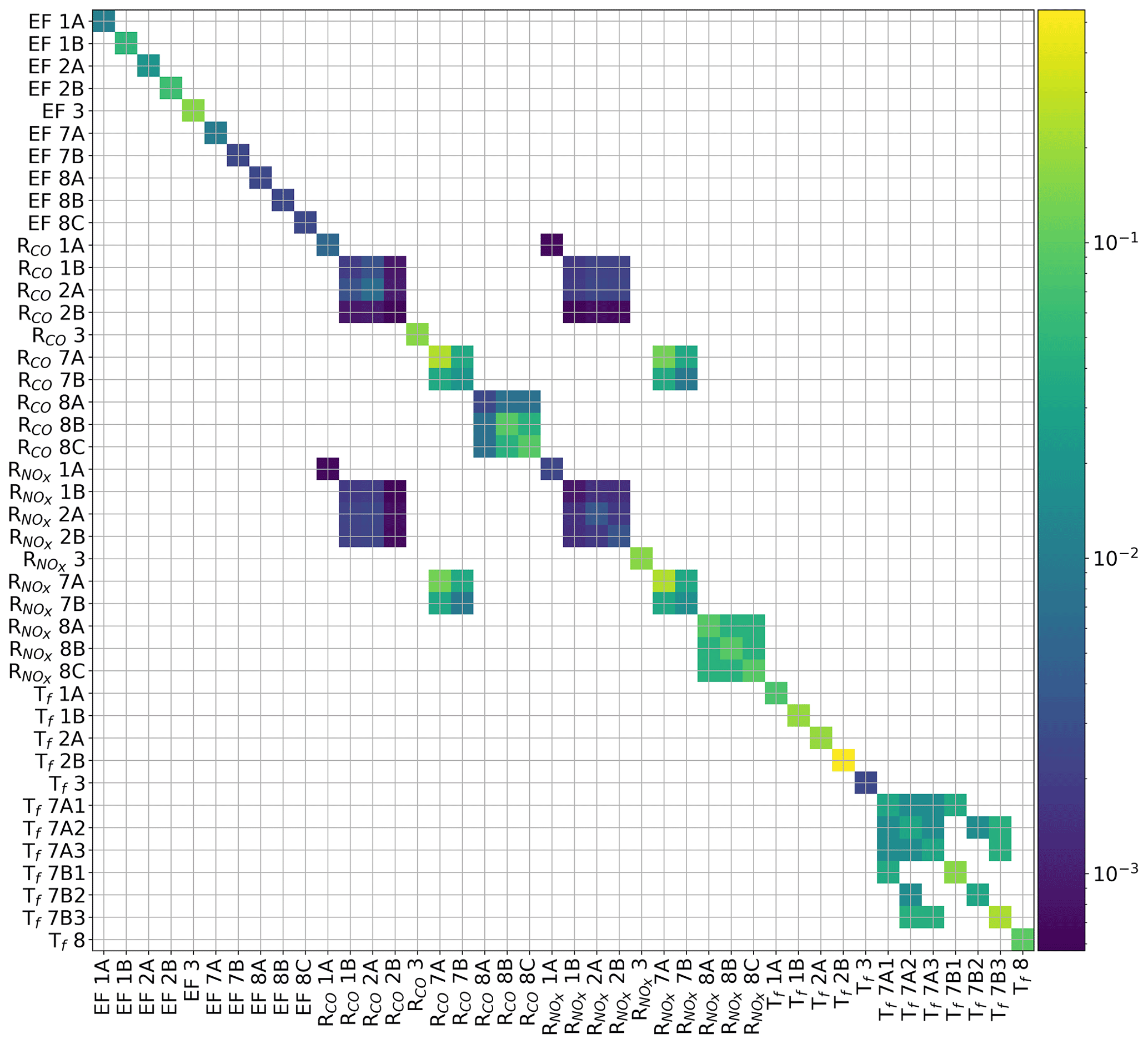
Figure A1Covariance matrix for all parameters in the emission model. For all covariances, we assume a correlation coefficient of 0.5. (Sub-)sectors are indicated with their short names as summarized in Table 1. Note that the time profiles of road traffic emissions are specified per road type (1 = highway, 2 = main road, 3 = urban road).
The daily time factor of gas combustion for households may be described in terms of two components. First, gas is used for warm water supply and cooking, which is relatively fixed. Second, gas is used for heating, which is strongly temperature dependent. The second component has previously been described using the degree day concept, from which the daily time factor can be defined as
where H is the heating degree day factor () based on the daily mean outside temperature at 2 m and a threshold temperature below which heating takes place. is the annual average heating degree day (). However, gas consumption related to warm water supply and cooking is largely independent of the outside temperature; therefore, a constant offset is included in the heating degree day factor:
where f is the constant offset, which is assigned equally to all days. The time factor can now be defined as
where the average heating degree day accounted for the constant offset .
Table B1Overview of the data used to create the temporal profiles presented in Sect. 2.1.2. The activity data represents the actual and the parameterizations are based on environmental variables or other proxies.
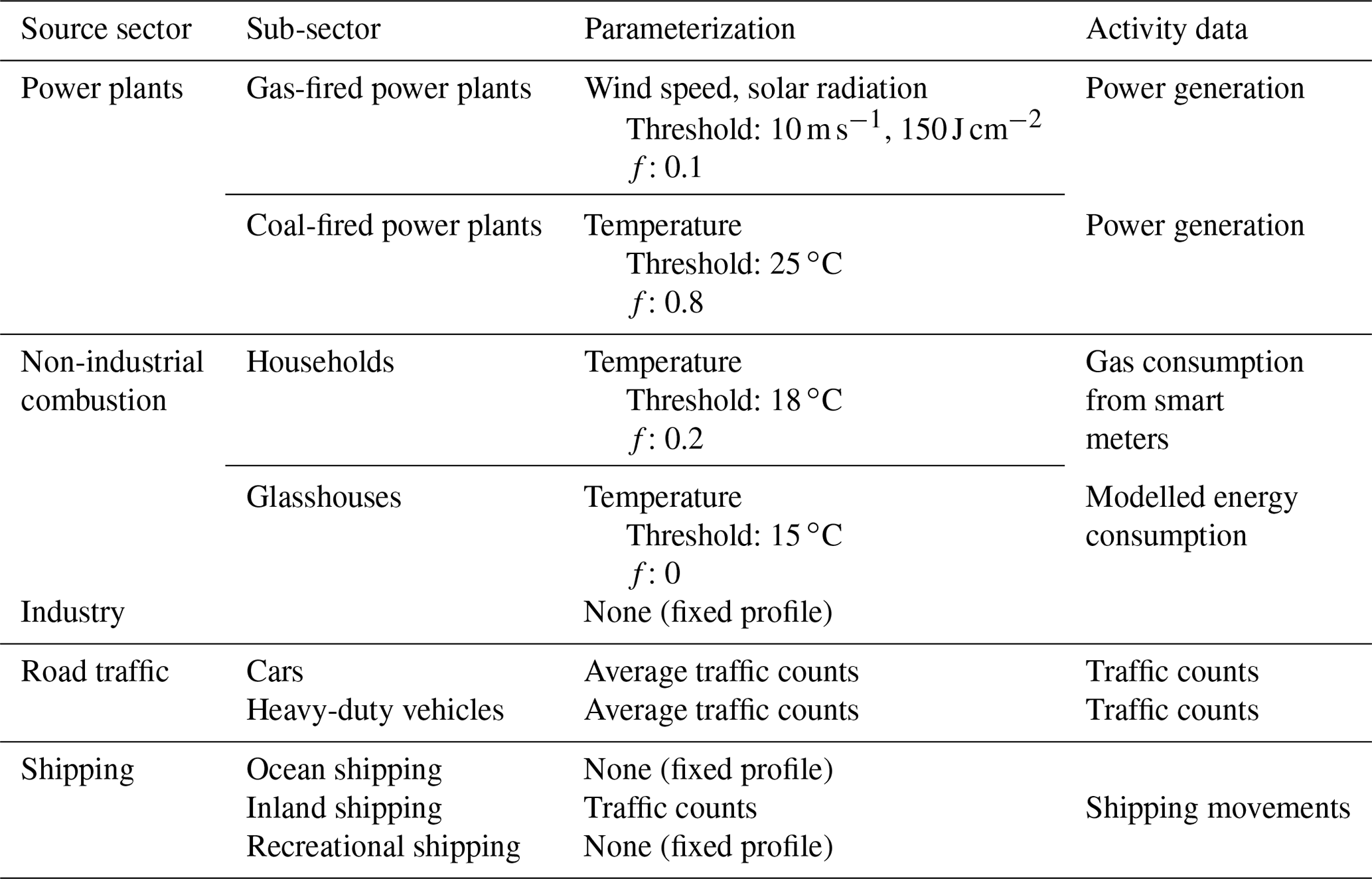
Equation (B3) is used for households and coal-fired power plants, whereas for glasshouses no constant offset is assumed and so Eq. (B1) is applied. For gas-fired power plants Eq. (B3) is used, but the temperature is replaced with average wind speed and solar radiation to match its function as backup for renewable energy supply:
where u is the wind speed (m s−1) and R the incoming solar radiation (J cm−2 h−1).
To generate a footprint with the WRF-STILT model, 75 particles are released at the observation site at the start of the back-trajectory and followed back in time. Given that the variability in hourly observations at an urban location is dominated by local signals, we construct back-trajectories spanning 6 h. This is based on the domain size, which could be covered within 6 h for typical wind speeds of 4 m s−1. Within this time frame, emissions can become well mixed throughout the boundary layer under normal daytime mixing conditions, such that emissions outside this range can be represented by a boundary inflow. Footprints are generated for each hour within the back-trajectory to account for hourly variations in the emissions. We drive STILT with meteorology from the WRF model (v3.5.1). The WRF model was set up with two nested domains (15 km×15 km and 3 km×3 km horizontal resolutions) and the STILT footprints have a 1 km×1 km resolution over the entire domain.
The OPS plume model keeps track of a plume trajectory, considering time-varying transport over longer distances (e.g. changes in wind direction and dispersion). If for a time step a specific plume affects the receptor, a Gaussian plume formulation is used to calculate the mole fraction caused by that source based on the true travel distance along the trajectory. We drive the model with the same WRF meteorology as STILT. Only primary meteorological variables (temperature, relative humidity, wind direction, wind speed, precipitation, global radiation) are prescribed; secondary variables (e.g. boundary layer height, friction velocity) are calculated by OPS itself and can differ from WRF. Similar to the WRF-STILT model, we assume an influence time of 6 h for our observations. However, in this case we run the OPS model forward from −6 h to the time of observation.
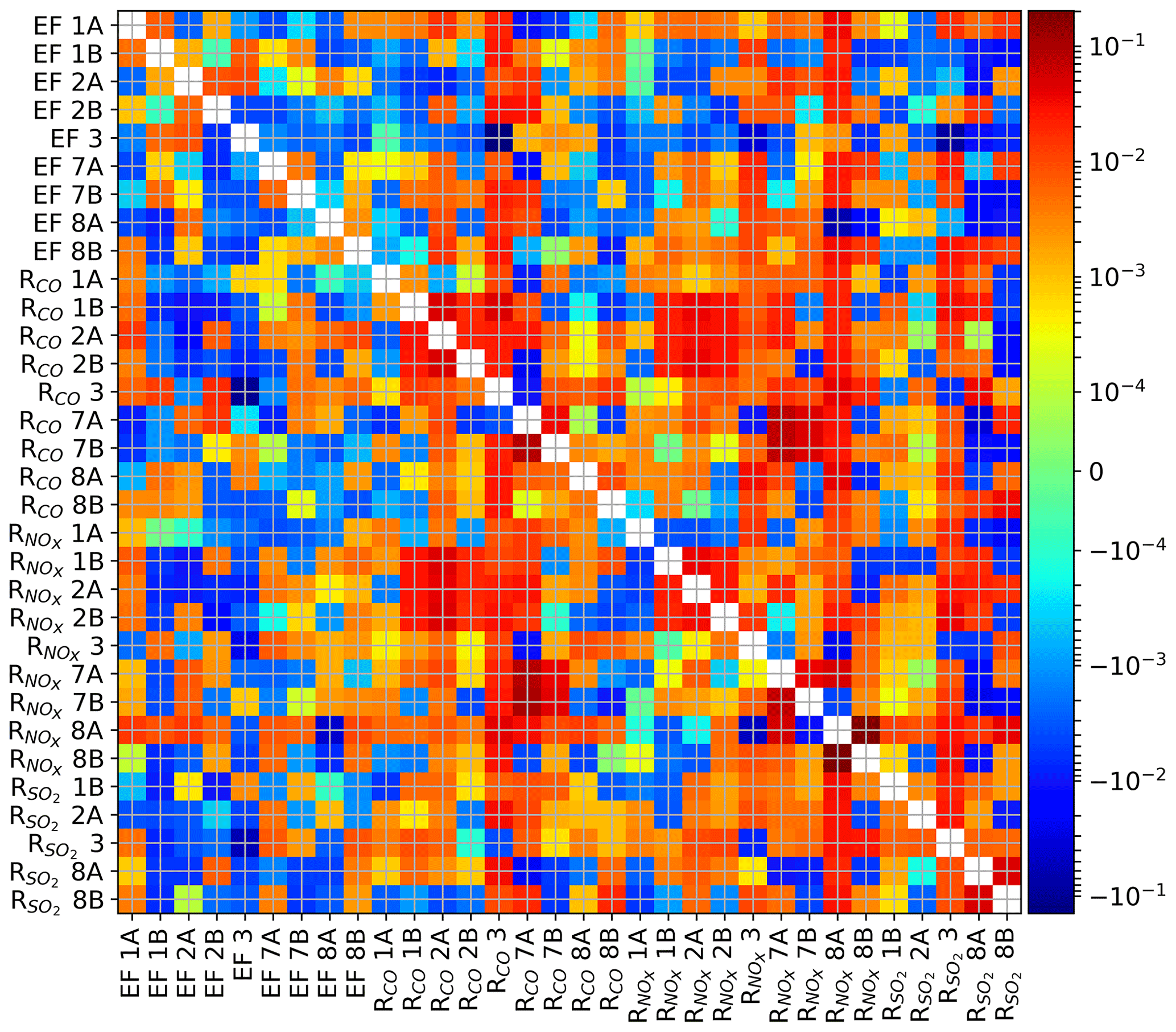
Figure D1Matrix showing the difference in correlation coefficient (r) between the CO2_only_no_propagation and No_ propagation run averaged for all 14 d, where positive differences indicate reduced parameter correlations when all tracers are included (No_propagation). (Sub-)sectors are indicated with their short names as summarized in Table 1. For some parameters, a strong reduction in parameter correlations is shown, indicating that with all tracers that parameter can be more easily separated from others, e.g. the emission factors of industry and coal-fired power plants (EF3 and EF1B).
CTDAS (v1.0) (van der Laan-Luijkx et al., 2017) is released under a GNU-GPL3.0 licence and forms the basis of the system described in this paper. Minor changes have been made to include the dynamic emission model. Revised code and the additional module used to describe the dynamic emission model and the creation of pseudo-observations is included in the Supplement, as is a script used for the emission uncertainty analysis (Monte Carlo simulation). Input data for the dynamic emission model are taken from open, online databases and are summarized in Appendix A, including their data sources. Example input files for CTDAS and the OPS model are also included in the Supplement.
The supplement related to this article is available online at: https://doi.org/10.5194/gmd-13-2695-2020-supplement.
The initial ideas were developed by WP, IS, HACDvdG, and MKvdM. IS and SNCD developed the dynamic emission model. IS and WP are responsible for setting up the inverse modelling experiments and prepared the article with contributions from all co-authors.
The authors declare that they have no conflict of interest.
This research has been supported by the European Union's Horizon 2020 programme (VERIFY (grant no. 776810)) and by EIT Climate-KIC project Carbocount-CITY (project no. APIN0029 2015-3.1-029 P040-04) and the EIT Climate-KIC Fellows programme (programme no. ARED0004 2013-1.1-008 P017-0x).
This paper was edited by Leena Järvi and reviewed by two anonymous referees.
Akaike, H.: A new look at the statistical model identification, in: Selected papers of Hirotugu Akaike. Springer Series in Statistics (Perspectives in Statistics), edited by: Parzen, E., Tanabe, K., and Kitagawa, G., Springer, New York, NY, 215–222, https://doi.org/10.1007/978-1-4612-1694-0_16, 1974.
Andres, R. J., Boden, T. A., and Higdon, D.: A new evaluation of the uncertainty associated with CDIAC estimates of fossil fuel carbon dioxide emission, Tellus B, 66, 23616, https://doi.org/10.3402/tellusb.v66.23616, 2014.
Andres, R. J., Boden, T. A., and Higdon, D. M.: Gridded uncertainty in fossil fuel carbon dioxide emission maps, a CDIAC example, Atmos. Chem. Phys., 16, 14979–14995, https://doi.org/10.5194/acp-16-14979-2016, 2016.
Angevine, W. M., Brioude, J., McKeen, S., and Holloway, J. S.: Uncertainty in Lagrangian pollutant transport simulations due to meteorological uncertainty from a mesoscale WRF ensemble, Geosci. Model Dev., 7, 2817–2829, https://doi.org/10.5194/gmd-7-2817-2014, 2014.
Asefi-Najafabady, S., Rayner, P. J., Gurney, K. R., McRobert, A., Song, Y., Coltin, K., Huang, J., Elvidge, C., and Baugh, K.: A multiyear, global gridded fossil fuel CO2 emission data product: Evaluation and analysis of results, J. Geophys. Res.-Atmos., 119, 10213–210231, https://doi.org/10.1002/2013jd021296, 2014.
Basu, S., Miller, J. B., and Lehman, S.: Separation of biospheric and fossil fuel fluxes of CO2 by atmospheric inversion of CO2 and 14CO2 measurements: Observation System Simulations, Atmos. Chem. Phys., 16, 5665–5683, https://doi.org/10.5194/acp-16-5665-2016, 2016.
Boon, A., Broquet, G., Clifford, D. J., Chevallier, F., Butterfield, D. M., Pison, I., Ramonet, M., Paris, J.-D., and Ciais, P.: Analysis of the potential of near-ground measurements of CO2 and CH4 in London, UK, for the monitoring of city-scale emissions using an atmospheric transport model, Atmos. Chem. Phys., 16, 6735–6756, https://doi.org/10.5194/acp-16-6735-2016, 2016.
Boschetti, F., Thouret, V., Maenhout, G. J., Totsche, K. U., Marshall, J., and Gerbig, C.: Multi-species inversion and IAGOS airborne data for a better constraint of continental-scale fluxes, Atmos. Chem. Phys., 18, 9225–9241, https://doi.org/10.5194/acp-18-9225-2018, 2018.
Bréon, F. M., Broquet, G., Puygrenier, V., Chevallier, F., Xueref-Remy, I., Ramonet, M., Dieudonné, E., Lopez, M., Schmidt, M., Perrussel, O., and Ciais, P.: An attempt at estimating Paris area CO2 emissions from atmospheric concentration measurements, Atmos. Chem. Phys., 15, 1707–1724, https://doi.org/10.5194/acp-15-1707-2015, 2015.
Brioude, J., Angevine, W. M., Ahmadov, R., Kim, S.-W., Evan, S., McKeen, S. A., Hsie, E.-Y., Frost, G. J., Neuman, J. A., Pollack, I. B., Peischl, J., Ryerson, T. B., Holloway, J., Brown, S. S., Nowak, J. B., Roberts, J. M., Wofsy, S. C., Santoni, G. W., Oda, T., and Trainer, M.: Top-down estimate of surface flux in the Los Angeles Basin using a mesoscale inverse modeling technique: assessing anthropogenic emissions of CO, NOx and CO2 and their impacts, Atmos. Chem. Phys., 13, 3661–3677, https://doi.org/10.5194/acp-13-3661-2013
Brophy, K., Graven, H., Manning, A. J., White, E., Arnold, T., Fischer, M. L., Jeong, S., Cui, X., and Rigby, M.: Characterizing uncertainties in atmospheric inversions of fossil fuel CO2 emissions in California, Atmos. Chem. Phys., 19, 2991–3006, https://doi.org/10.5194/acp-19-2991-2019, 2019.
Broquet, G., Bréon, F.-M., Renault, E., Buchwitz, M., Reuter, M., Bovensmann, H., Chevallier, F., Wu, L., and Ciais, P.: The potential of satellite spectro-imagery for monitoring CO2 emissions from large cities, Atmos. Meas. Tech., 11, 681–708, https://doi.org/10.5194/amt-11-681-2018, 2018.
Chevallier, F., Viovy, N., Reichstein, M., and Ciais, P.: On the assignment of prior errors in Bayesian inversions of CO2 surface fluxes, Geophys. Res. Lett., 33, L13802, https://doi.org/10.1029/2006GL026496, 2006.
Ciais, P., Paris, J. D., Marland, G., Peylin, P., Piao, S. L., Levin, I., Pregger, T., Scholz, Y., Friedrich, R., Rivier, L., Houwelling, S., and Schulze, E. D.: The European carbon balance. Part 1: Fossil fuel emissions, Glob. Change Biol., 16, 1395–1408, https://doi.org/10.1111/j.1365-2486.2009.02098.x, 2010.
Deng, A., Lauvaux, T., Davis, K. J., Gaudet, B. J., Miles, N., Richardson, S. J., Wu, K., Sarmiento, D. P., Hardesty, R. M., Bonin, T. A., Brewer, W. A., and Gurney, K. R.: Toward reduced transport errors in a high resolution urban CO2 inversion system, Elementa (Wash. D.C.), 5, 20, https://doi.org/10.1525/elementa.133, 2017.
Denier van der Gon, H. A. C., Hendriks, C., Kuenen, J., Segers, A., and Visschedijk, A.: Description of current temporal emission patterns and sensitivity of predicted AQ for temporal emission patterns, Report, TNO, Utrecht, 2011.
Djuricin, S., Pataki, D. E., and Xu, X.: A comparison of tracer methods for quantifying CO2 sources in an urban region, J. Geophys. Res., 115, D11303, https://doi.org/10.1029/2009JD012236, 2010.
Fauser, P., Sørensen, P. B., Nielsen, M., Winther, M., Plejdrup, M. S., Hoffmann, L., Gyldenkærne, S., Mikkelsen, M. H., Albrektsen, R., Lyck, E., Thomsen, M., Hjelgaard, K., and Nielsen, O.-K.: Monte Carlo (Tier 2) uncertainty analysis of Danish Greenhouse gas emission inventory, Greenhouse Gas Measurement and Management, 1, 145–160, https://doi.org/10.1080/20430779.2011.621949, 2011.
Fischer, M. L., Parazoo, N., Brophy, K., Cui, X., Jeong, S., Liu, J., Keeling, R., Taylor, T. E., Gurney, K., Oda, T., and Graven, H.: Simulating estimation of California fossil fuel and biosphere carbon dioxide exchanges combining in situ tower and satellite column observations, J. Geophys. Res.-Atmos., 122, 3653–3671, https://doi.org/10.1002/2016jd025617, 2017.
Gerbig, C., Lin, J. C., Wofsy, S. C., Daube, B. C., Andrews, A. E., Stephens, B. B., Bakwin, P. S., and Grainger, C. A.: Toward constraining regional-scale fluxes of CO2 with atmospheric observations over a continent: 2. Analysis of COBRA data using a receptor-oriented framework, J. Geophys. Res., 108, 4757, https://doi.org/10.1029/2003JD003770, 2003.
Göckede, M., Turner, D. P., Michalak, A. M., Vickers, D., and Law, B. E.: Sensitivity of a subregional scale atmospheric inverse CO2 modeling framework to boundary conditions, J. Geophys. Res., 115, D24112, https://doi.org/10.1029/2010JD014443, 2010.
Graven, H., Fischer, M. L., Lueker, T., Jeong, S., Guilderson, T. P., Keeling, R. F., Bambha, R., Brophy, K., Callahan, W., Cui, X., Frankenberg, C., Gurney, K. R., LaFranchi, B. W., Lehman, S. J., Michelsen, H., Miller, J. B., Newman, S., Paplawsky, W., Parazoo, N. C., Sloop, C., and Walker, S. J.: Assessing fossil fuel CO2 emissions in California using atmospheric observations and models, Environ. Res. Lett., 13, 065007, https://doi.org/10.1088/1748-9326/aabd43, 2018.
Gurney, K. R., Patarasuk, R., Liang, J., Song, Y., O'Keeffe, D., Rao, P., Whetstone, J. R., Duren, R. M., Eldering, A., and Miller, C.: The Hestia fossil fuel CO2 emissions data product for the Los Angeles megacity (Hestia-LA), Earth Syst. Sci. Data, 11, 1309–1335, https://doi.org/10.5194/essd-11-1309-2019, 2019.
He, W., van der Velde, I. R., Andrews, A. E., Sweeney, C., Miller, J., Tans, P., van der Laan-Luijkx, I. T., Nehrkorn, T., Mountain, M., Ju, W., Peters, W., and Chen, H.: CTDAS-Lagrange v1.0: a high-resolution data assimilation system for regional carbon dioxide observations, Geosci. Model Dev., 11, 3515–3536, https://doi.org/10.5194/gmd-11-3515-2018, 2018.
Hirth, L., Mühlenpfordt, J., and Bulkeley, M.: The ENTSO-E Transparency Platform – A review of Europe's most ambitious electricity data platform, Appl. Energ., 225, 1054–1067, https://doi.org/10.1016/j.apenergy.2018.04.048, 2018.
Hogue, S., Marland, E., Andres, R. J., Marland, G., and Woodard, D.: Uncertainty in gridded CO2 emissions estimates, Earth's Future, 4, 225–239, https://doi.org/10.1002/2015EF000343, 2016.
Huijnen, V., Williams, J., van Weele, M., van Noije, T., Krol, M., Dentener, F., Segers, A., Houweling, S., Peters, W., de Laat, J., Boersma, F., Bergamaschi, P., van Velthoven, P., Le Sager, P., Eskes, H., Alkemade, F., Scheele, R., Nédélec, P., and Pätz, H.-W.: The global chemistry transport model TM5: description and evaluation of the tropospheric chemistry version 3.0, Geosci. Model Dev., 3, 445–473, https://doi.org/10.5194/gmd-3-445-2010, 2010.
Hutchins, M. G., Colby, J. D., Marland, G., and Marland, E.: A comparison of five high-resolution spatially-explicit, fossil-fuel, carbon dioxide emission inventories for the United States, Mitig. Adapt. Strat. Gl., 22, 947–972, https://doi.org/10.1007/s11027-016-9709-9, 2017.
IEA: World Energy Outlook 2008, International Energy Agency, Paris, 2008.
Jansen, B. I.: Vernieuwd emissiemodel houtkachels, TNO-rapport, TNO 2016 R10318, 28 pp., TNO, Delft, 2016.
Jun, P., Gillenwater, M., and Barbour, W.: CO2, CH4, and N2O emissions from transportation – water-borne navigation, in: Good Practice Guidance and Uncertainty Management in National Greenhouse Gas Inventories, Intergovernmental Panel on Climate Change, Paris, France, 71–92, 2000.
Kuenen, J. J. P., Visschedijk, A. J. H., Jozwicka, M., and Denier van der Gon, H. A. C.: TNO-MACC_II emission inventory; a multi-year (2003–2009) consistent high-resolution European emission inventory for air quality modelling, Atmos. Chem. Phys., 14, 10963–10976, https://doi.org/10.5194/acp-14-10963-2014, 2014.
Kuhlmann, G., Broquet, G., Marshall, J., Clément, V., Löscher, A., Meijer, Y., and Brunner, D.: Detectability of CO2 emission plumes of cities and power plants with the Copernicus Anthropogenic CO2 Monitoring (CO2M) mission, Atmos. Meas. Tech., 12, 6695–6719, https://doi.org/10.5194/amt-12-6695-2019, 2019.
LaFranchi, B. W., Pétron, G., Miller, J. B., Lehman, S. J., Andrews, A. E., Dlugokencky, E. J., Hall, B., Miller, B. R., Montzka, S. A., Neff, W., Novelli, P. C., Sweeney, C., Turnbull, J. C., Wolfe, D. E., Tans, P. P., Gurney, K. R., and Guilderson, T. P.: Constraints on emissions of carbon monoxide, methane, and a suite of hydrocarbons in the Colorado Front Range using observations of 14CO2, Atmos. Chem. Phys., 13, 11101–11120, https://doi.org/10.5194/acp-13-11101-2013, 2013.
Lauvaux, T., Miles, N. L., Richardson, S. J., Deng, A., Stauffer, D. R., Davis, K. J., Jacobson, G., Rella, C., Calonder, G. P., and Decola, P. L.: Urban emissions of CO2 from Davos, Switzerland: The first real-time monitoring system using an atmospheric inversion technique, J. Appl. Meteorol. Clim., 52, 2654–2668, https://doi.org/10.1175/JAMC-D-13-038.1, 2013.
Lauvaux, T., Miles, N. L., Deng, A., Richardson, S. J., Cambaliza, M. O., Davis, K. J., Gaudet, B., Gurney, K. R., Huang, J., O'Keefe, D., Song, Y., Karion, A., Oda, T., Patarasuk, R., Razlivanov, I., Sarmiento, D., Shepson, P., Sweeney, C., Turnbull, J., and Wu, K.: High-resolution atmospheric inversion of urban CO2 emissions during the dormant season of the Indianapolis Flux Experiment (INFLUX), J. Geophys. Res.-Atmos., 121, 5213–5236, https://doi.org/10.1002/2015jd024473, 2016.
Levin, I. and Karstens, U.: Inferring high-resolution fossil fuel CO2 records at continental sites from combined 14CO2 and CO observations, Tellus B, 59, 245–250, https://doi.org/10.1111/j.1600-0889.2006.00244.x, 2007.
Liander: Innovatie & Diensten: Open data, available at: https://www.liander.nl/over-liander/innovatie/open-data/data, last access: February 2018.
Lin, J. C., Gerbig, C., Wofsy, S. C., Andrews, A. E., Daube, B. C., Davis, K. J., and Grainger, C. A. C.: A near-field tool for simulating the upstream influence of atmospheric observations: The Stochastic Time-Inverted Lagrangian Transport (STILT) model, J. Geophys. Res., 108, 4493, https://doi.org/10.1029/2002jd003161, 2003.
Lindenmaier, R., Dubey, M. K., Henderson, B. G., Butterfield, Z. T., Herman, J. R., Rahn, T., and Lee, S. H.: Multiscale observations of CO2, 13CO2, and pollutants at Four Corners for emission verification and attribution, P. Natl. Acad. Sci. USA, 111, 8386–8391, 2014.
Lopez, M., Schmidt, M., Delmotte, M., Colomb, A., Gros, V., Janssen, C., Lehman, S. J., Mondelain, D., Perrussel, O., Ramonet, M., Xueref-Remy, I., and Bousquet, P.: CO, NOx and 13CO2 as tracers for fossil fuel CO2: results from a pilot study in Paris during winter 2010, Atmos. Chem. Phys., 13, 7343–7358, https://doi.org/10.5194/acp-13-7343-2013
McKain, K., Wofsy, S. C., Nehrkorn, T., Eluszkiewicz, J., Ehleringer, J. R., and Stephens, B. B.: Assessment of ground-based atmospheric observations for verification of greenhouse gas emissions from an urban region, P. Natl. Acad. Sci. USA, 109, 8423–8428, 2012.
Meirink, J. F., Bergamaschi, P., Frankenberg, C., d'Amelio, M. T. S., Dlugokencky, E. J., Gatti, L. V., Houweling, S., Miller, J. B., Röckmann, T., Villani, M. G., and Krol, M. C.: Four-dimensional variational data assimilation for inverse modeling of atmospheric methane emissions: Analysis of SCIAMACHY observations, J. Geophys. Res., 113, D17301, https://doi.org/10.1029/2007jd009740, 2008.
Miller, J. B., Lehman, S. J., Montzka, S. A., Sweeney, C., Miller, B. R., Karion, A., Wolak, C., Dlugokencky, E. J., Southon, J., Turnbull, J. C., and Tans, P. P.: Linking emissions of fossil fuel CO2 and other anthropogenic trace gases using atmospheric 14CO2, J. Geophys. Res., 117, D08302, https://doi.org/10.1029/2011jd017048, 2012.
Monni, S., Syri, S., and Savolainen, I.: Uncertainties in the Finnish greenhouse gas emission inventory, Environ. Sci. Policy, 7, 87–98, https://doi.org/10.1016/j.envsci.2004.01.002, 2004.
Mues, A., Kuenen, J., Hendriks, C., Manders, A., Segers, A., Scholz, Y., Hueglin, C., Builtjes, P., and Schaap, M.: Sensitivity of air pollution simulations with LOTOS-EUROS to the temporal distribution of anthropogenic emissions, Atmos. Chem. Phys., 14, 939–955, https://doi.org/10.5194/acp-14-939-2014, 2014.
Nakicenovic, N., Alcamo, J., Davis, G., De Vries, B., Fenhann, J., Gaffin, S., Gregory, K., Grübler, A., Jung, T. Y., Kram, T., La Rovere, E. L., Michaelis, L., Mori, S., Morita, T., Pepper, W., Pitcher, H., Price, L., Riahi, K., Roehrl, A., Rogner, H.-H., Sankovski, A., Schlesinger, M., Shukla, P., Smith, S., Swart, R., Van Rooijen, S., Victor, N., and Dadi, Z.: IPCC Special Report on Emissions Scenarios, edited by: Calvo, E., Chadwick, M., Ishiumi, Y., and Parikh, J., Cambridge University Press, Cambridge, UK, 599 pp., 2000.
Nassar, R., Napier-Linton, L., Gurney, K. R., Andres, R. J., Oda, T., Vogel, F. R., and Deng, F.: Improving the temporal and spatial distribution of CO2 emissions from global fossil fuel emission data sets, J. Geophys. Res.-Atmos., 118, 917–933, https://doi.org/10.1029/2012jd018196, 2013.
Nathan, B., Lauvaux, T., Turnbull, J., and Gurney, K.: Investigations into the use of multi-species measurements for source apportionment of the Indianapolis fossil fuel CO2 signal, Elementa, 6, 21, https://doi.org/10.1525/elementa.131, 2018.
Nehrkorn, T., Eluszkiewicz, J., Wofsy, S. C., Lin, J. C., Gerbig, C., Longo, M., and Freitas, S.: Coupled weather research and forecasting-stochastic time-inverted lagrangian transport (WRF-STILT) model, Meteorol. Atmos. Phys., 107, 51–64, https://doi.org/10.1007/s00703-010-0068-x, 2010.
Netherlands PRTR: Netherlands Pollutant Release & Transfer Register: http://www.emissieregistratie.nl/, last access: March 2018.
Palmer, P. I., O'Doherty, S., Allen, G., Bower, K., Bösch, H., Chipperfield, M. P., Connors, S., Dhomse, S., Feng, L., Finch, D. P., Gallagher, M. W., Gloor, E., Gonzi, S., Harris, N. R. P., Helfter, C., Humpage, N., Kerridge, B., Knappett, D., Jones, R. L., Le Breton, M., Lunt, M. F., Manning, A. J., Matthiesen, S., Muller, J. B. A., Mullinger, N., Nemitz, E., O'Shea, S., Parker, R. J., Percival, C. J., Pitt, J., Riddick, S. N., Rigby, M., Sembhi, H., Siddans, R., Skelton, R. L., Smith, P., Sonderfeld, H., Stanley, K., Stavert, A. R., Wenger, A., White, E., Wilson, C., and Young, D.: A measurement-based verification framework for UK greenhouse gas emissions: an overview of the Greenhouse gAs Uk and Global Emissions (GAUGE) project, Atmos. Chem. Phys., 18, 11753–11777, https://doi.org/10.5194/acp-18-11753-2018, 2018.
Peters, W., Miller, J. B., Whitaker, J., Denning, A. S., Hirsch, A., Krol, M. C., Zupanski, D., Bruhwiler, L., and Tans, P. P.: An ensemble data assimilation system to estimate CO2 surface fluxes from atmospheric trace gas observations, J. Geophys. Res., 110, D24304, https://doi.org/10.1029/2005JD006157, 2005.
Peters, W., Krol, M. C., Van der Werf, G. R., Houweling, S., Jones, C. D., Hughes, J., Schaefer, K., Masarie, K. A., Jacobson, A. R., Miller, J. B., Cho, C. H., Ramonet, M., Schmidt, M., Ciattaglia, L., Apadula, F., Heltai, D., Meinhardt, F., Di Sarra, A. G., Piacentino, S., Sferlazzo, D., Aalto, T., Hatakka, J., Ström, J., Haszpra, L., Meijer, H. A. J., Van der Laan, S., Neubert, R. E. M., Jordan, A., Rodó, X., Morguí, J. A., Vermeulen, A. T., Popa, E., Rozanski, K., Zimnoch, M., Manning, A. C., Leuenberger, M., Uglietti, C., Dolman, A. J., Ciais, P., Heimann, M., and Tans, P.: Seven years of recent European net terrestrial carbon dioxide exchange constrained by atmospheric observations, Glob. Change Biol., 16, 1317–1337, https://doi.org/10.1111/j.1365-2486.2009.02078.x, 2010.
Ramírez, A. R., De Keizer, C., and Van der Sluijs, J. P.: Monte Carlo analysis of uncertainties in the Netherlands Greenhouse Gas Emission Inventory for 1990–2004, Copernicus Institute for Sustainable Development and Innovation, Utrecht, Report no: NWS-E-2006-58, 111 pp., 2006.
Rao, P., Gurney, K. R., Patarasuk, R., Song, Y., Miller, C. E., Duren, R. M., and Eldering, A.: Spatio-temporal Variations in on-road CO2 Emissions in the Los Angeles Megacity, AIMS Geosciences, 3, 239–267, https://doi.org/10.3934/geosci.2017.2.239, 2017.
Raupach, M. R., Marland, G., Ciais, P., Le Quéré, C., Canadell, J. G., Klepper, G., and Field, C. B.: Global and regional drivers of accelerating CO2 emissions, P. Natl. Acad. Sci. USA, 104, 10288–10293, https://doi.org/10.1073/pnas.0700609104, 2007.
Rayner, P. J., Raupach, M. R., Paget, M., Peylin, P., and Koffi, E.: A new global gridded data set of CO2 emissions from fossil fuel combustion: Methodology and evaluation, J. Geophys. Res., 115, D19306, https://doi.org/10.1029/2009jd013439, 2010.
Sargent, M., Barrera, Y., Nehrkorn, T., Hutyra, L. R., Gately, C. K., Jones, T., McKain, K., Sweeney, C., Hegarty, J., Hardiman, B., Wang, J. A., and Wofsy, S. C.: Anthropogenic and biogenic CO2 fluxes in the Boston urban region, P. Natl. Acad. Sci. USA, 115, 7491–7496, https://doi.org/10.1073/pnas.1803715115, 2018.
Sauter, F., Van Zanten, M., Van der Swaluw, E., Aben, J., De Leeuw, F., and Van Jaarsveld, H.: The OPS-model. Description of OPS 4.5.0, National Institute for Public Health and the Environment (RIVM), Bilthoven, 115 pp., 2016.
Staufer, J., Broquet, G., Bréon, F.-M., Puygrenier, V., Chevallier, F., Xueref-Rémy, I., Dieudonné, E., Lopez, M., Schmidt, M., Ramonet, M., Perrussel, O., Lac, C., Wu, L., and Ciais, P.: The first 1-year-long estimate of the Paris region fossil fuel CO2 emissions based on atmospheric inversion, Atmos. Chem. Phys., 16, 14703–14726, https://doi.org/10.5194/acp-16-14703-2016, 2016.
Su, H., Yang, Z. L., Niu, G. Y., and Wilson, C. R.: Parameter estimation in ensemble based snow data assimilation: A synthetic study, Adv. Water Resour., 34, 407–416, https://doi.org/10.1016/j.advwatres.2010.12.002, 2011.
Super, I., Denier van der Gon, H. A. C., van der Molen, M. K., Sterk, H. A. M., Hensen, A., and Peters, W.: A multi-model approach to monitor emissions of CO2 and CO from an urban–industrial complex, Atmos. Chem. Phys., 17, 13297–13316, https://doi.org/10.5194/acp-17-13297-2017, 2017a.
Super, I., Denier van der Gon, H. A. C., Visschedijk, A. J. H., Moerman, M. M., Chen, H., Van der Molen, M. K., and Peters, W.: Interpreting continuous in-situ observations of carbon dioxide and carbon monoxide in the urban port area of Rotterdam, Atmos. Pollut. Res., 8, 174–187, https://doi.org/10.1016/j.apr.2016.08.008, 2017b.
Super, I., Dellaert, S. N. C., Visschedijk, A. J. H., and Denier van der Gon, H. A. C.: Uncertainty analysis of a European high-resolution emission inventory of CO2 and CO to support inverse modelling and network design, Atmos. Chem. Phys., 20, 1795–1816, https://doi.org/10.5194/acp-20-1795-2020, 2020.
Terrenoire, E., Bessagnet, B., Rouïl, L., Tognet, F., Pirovano, G., Létinois, L., Beauchamp, M., Colette, A., Thunis, P., Amann, M., and Menut, L.: High-resolution air quality simulation over Europe with the chemistry transport model CHIMERE, Geosci. Model Dev., 8, 21–42, https://doi.org/10.5194/gmd-8-21-2015, 2015.
Tolk, L. F., Meesters, A. G. C. A., Dolman, A. J., and Peters, W.: Modelling representation errors of atmospheric CO2 mixing ratios at a regional scale, Atmos. Chem. Phys., 8, 6587–6596, https://doi.org/10.5194/acp-8-6587-2008, 2008.
Turnbull, J. C., Miller, J. B., Lehman, S. J., Tans, P. P., Sparks, R. J., and Southon, J.: Comparison of 14CO2, CO, and SF6 as tracers for recently added fossil fuel CO2 in the atmosphere and implications for biological CO2 exchange, Geophys. Res. Lett., 33, L01817, https://doi.org/10.1029/2005GL024213, 2006.
Turnbull, J. C., Sweeney, C., Karion, A., Newberger, T., Lehman, S. J., Tans, P. P., Davis, K. J., Lauvaux, T., Miles, N. L., Richardson, S. J., Cambaliza, M. O., Shepson, P. B., Gurney, K., Patarasuk, R., and Razlivanov, I.: Toward quantification and source sector identification of fossil fuel CO2 emissions from an urban area: Results from the INFLUX experiment, J. Geophys. Res.-Atmos., 120, 292–312, https://doi.org/10.1002/2014jd022555, 2015.
UNFCCC: Paris Agreement, UNFCCC, NY, United States, 2015.
van der Laan-Luijkx, I. T., van der Velde, I. R., van der Veen, E., Tsuruta, A., Stanislawska, K., Babenhauserheide, A., Zhang, H. F., Liu, Y., He, W., Chen, H., Masarie, K. A., Krol, M. C., and Peters, W.: The CarbonTracker Data Assimilation Shell (CTDAS) v1.0: implementation and global carbon balance 2001–2015, Geosci. Model Dev., 10, 2785–2800, https://doi.org/10.5194/gmd-10-2785-2017, 2017.
Van der Laan, S., Van der Laan-Luijkx, I. T., Zimmermann, L., Conen, F., and Leuenberger, M.: Net CO2 surface emissions at Bern, Switzerland inferred from ambient observations of CO2, δ(O2∕N2), and 222Rn using a customized radon tracer inversion, J. Geophys. Res.-Atmos., 119, 1580–1591, https://doi.org/10.1002/2013JD020307, 2014.
Van Jaarsveld, J. A.: The Operational Priority Substances model. Description and validation of OPS-Pro 4.1, National Institute for Public Health and the Environment, Bilthoven, Report no.: 500045001/2004, 156 pp., 2004.
Vogel, F. R., Thiruchittampalam, B., Theloke, J., Kretschmer, R., Gerbig, C., Hammer, S., and Levin, I.: Can we evaluate a fine-grained emission model using high-resolution atmospheric transport modelling and regional fossil fuel CO2 observations?, Tellus B, 65, 18681, https://doi.org/10.3402/tellusb.v65i0.18681, 2013.
Wang, Y., Broquet, G., Ciais, P., Chevallier, F., Vogel, F., Wu, L., Yin, Y., Wang, R., and Tao, S.: Potential of European 14CO2 observation network to estimate the fossil fuel CO2 emissions via atmospheric inversions, Atmos. Chem. Phys., 18, 4229–4250, https://doi.org/10.5194/acp-18-4229-2018, 2018.
Whitaker, J. S. and Hamill, T. M.: Ensemble data assimilation without perturbed observations, Mon. Weather Rev., 130, 1913–1924, https://doi.org/10.1175/1520-0493(2002)130<1913:EDAWPO>2.0.CO;2, 2002.
Zhou, Y., and Gurney, K. R.: Spatial relationships of sector-specific fossil fuel CO2 emissions in the United States, Global Biogeochem. Cy., 25, GB3002, https://doi.org/10.1029/2010gb003822, 2011.
- Abstract
- Introduction
- Methods
- Results
- Discussion
- Conclusions
- Appendix A: Emission model input data and uncertainties
- Appendix B: Temporal profiles
- Appendix C: Observation operator
- Appendix D
- Code and data availability
- Author contributions
- Competing interests
- Financial support
- Review statement
- References
- Supplement