2.1 Satellite data

The spatially explicit estimates of AGB were based on the radar backscattered intensity recorded by the Phased Array-type L-band Synthetic Aperture Radar (PALSAR) instrument, on board the Advanced Land Observing Satellite (ALOS) satellite, and the Advanced Synthetic Aperture Radar (ASAR) instrument operating at C-band, on board the Environmental Satellite (Envisat) (Sect. S1 in the Supplement). In addition, lidar-based metrics and surface reflectances were used throughout the process of biomass estimation.

ALOS PALSAR was an active microwave sensor operating at L-band (wavelength of 23 cm). Between 2006 and 2011, PALSAR acquired images in the Fine Beam Dual (FBD) polarization mode with 20 m spatial resolution. Image acquisition followed a predefined observation scenario with the aim of achieving spatially and temporally consistent large-scale observational datasets (Rosenqvist et al., 2007). Summertime acquisitions from the FBD mode (mostly May to October) were used by the Japan Aerospace Exploration Agency (JAXA) to generate yearly mosaics of the radar backscatter for each year between 2007 and 2010 (Shimada, 2010). Each image was orthorectified and radiometrically terrain-corrected to gamma0 (Shimada, 2010). The mosaics are publicly available and are provided in the form of image tiles of $\mathrm{1}{}^{\circ }\times \mathrm{1}{}^{\circ }$ in latitude and longitude, resampled to a grid with a pixel spacing of 0.000225^∘. In this study, we used the mosaics of the co-polarized horizontal-transmit horizontal-receive (HH) and cross-polarized horizontal-transmit vertical-receive (HV) backscatter images. Images from 14 728 tiles were used to estimate biomass; 96 image tiles showing evident radiometric offsets with respect to adjacent ones, due for example to different environmental conditions (e.g. frozen vs. unfrozen conditions), were manually replaced with the corresponding image tile from the mosaic of 2009. This replacement ensured homogeneity of the L-band backscatter dataset across all landscapes.

Envisat ASAR was an active microwave sensor acquiring images at C-band (wavelength of 6 cm) between 2002 and 2012. ASAR operated in four different modes over land, with a spatial resolution of 30 m (Image Mode, IM, and Alternating Polarization Mode, APM), 150 m (Wide Swath Mode, WSM), and 1000 m (Global Monitoring Mode, GMM). Approximately 80 % of the total number of observations consisted of GM observations. We processed the entire dataset of ASAR images of the synthetic aperture radar (SAR) backscatter made available by the European Space Agency (ESA) through the Grid Processing on Demand platform to stacks of terrain-geocoded, pixel-area-normalized, and speckle-filtered images (Santoro et al., 2015b). Images acquired with the IM and WSM were geocoded to a pixel size of 0.0013888^∘ in latitude and longitude, corresponding to an area on the ground of roughly 150 m×150 m at the Equator. Images acquired with the GMM were geocoded to a pixel size of 0.01^∘ in latitude and longitude, corresponding to an area on the ground of approximately 1000 m×1000 m at the Equator. To obtain global full coverage, the IM and WSM images were further averaged and resampled to the pixel size of the GMM dataset to form a single 1 km dataset of C-band backscatter observations. Each image was divided into tiles of $\mathrm{2}{}^{\circ }\times \mathrm{2}{}^{\circ }$ in latitude and longitude. For this study, we used all Envisat ASAR images acquired in 2010 and 2011. The density of the observations in time (Fig. S1 in the Supplement) decreased from the polar latitudes, with several observations per day, to the tropical latitudes, with approximately 200 observations on average over 2 years. Areas with a small number of observations correspond to regions seldom imaged during the lifetime of the Envisat mission (e.g. New Zealand, Japan) or imaged only at high resolution when the overlap of images from the adjacent orbital track was null (e.g. California, western Amazon).

The parameterization of the biomass retrieval models relating biomass to SAR backscatter observations was supported by the GLA14 data product of the Geoscience Laser Altimeter System (GLAS) on board the Ice Cloud and Land Elevation Satellite (ICESat) that operated between 2003 and 2009. GLA14 represented the waveforms over land only in the form of the parameters of a multi-Gaussian model fitted to the raw waveforms (Hofton et al., 2000), thus containing information about the vertical structure of vegetation. Because GLAS observations consisted of approximately 65 m large footprints acquired every 170 m along-track with a distance between tracks of the order of 60 km, the GLA14 dataset was not dense enough to allow direct spatially explicit estimates of biomass. Here, we used the entire archive of GLA14 data products, provided by the National Snow and Ice Data Centre (NSIDC), to estimate forest height after filtering for footprints affected by topography and various noise sources in the waveforms (Los et al., 2012; Simard et al., 2011). In addition, we computed an estimate of the canopy density for each footprint as the ratio of energy received from the canopy (i.e. returns from above the ground peak) to the total energy received. Our database of GLAS-based metrics consisted of 26.5 million footprints homogeneously distributed over all vegetated surfaces. While the SAR observations were used as predictors in the retrieval model (Sect. 3), the lidar observations supported the estimation of parameters of the retrieval model that are time-invariant such as forest transmissivity (Sect. 3). Herewith, the time difference between the SAR imagery (2010) and the lidar observations (2003–2009) did not impact the retrieval.

Global reflectances of Landsat 7 images (bands 3, 4, 5, and 7) acquired in 2010 were used to rescale biomass estimates from ASAR to the pixel size of the ALOS PALSAR dataset. The dataset was available in the form of a mosaic from the USGS website (Hansen et al., 2013). The square pixels of the mosaic had a spacing of 0.00027^∘, i.e. roughly 30 m at the Equator. The dataset was downloaded from Google Earth Engine and resampled with the nearest neighbour interpolation technique to the geometry of the ALOS PALSAR dataset.

Figure 1Flowchart of the AGB retrieval approach.

Download

2.2 AGB estimation

Unlike investigations that directly relate AGB to the remote sensing data (Lu et al., 2016; Santoro and Cartus, 2018), we estimated the density of the woody volume, referred to as growing stock volume (GSV; unit: m³ ha⁻¹), from which AGB is then computed, for three reasons. First, the signal backscattered by a forest is primarily affected by the density and to some degree the height of the trees (Santoro et al., 2015a). However, the short wavelength of the radar instruments means that only the upper part of the volume is seen so that an estimate of GSV (or AGB) would be the result of an inference from the SAR observation. Second, it has not been demonstrated that the SAR backscatter at C- and L-band is sensitive to the wood density of trees for a given level of GSV, thus not providing experimental support to a direct estimation of AGB. Without such evidence, it is preferable to estimate a forest structural parameter from the SAR backscatter and convert it to AGB using a separate layer combining the wood density and the stem-to-total biomass expansion factor, which does not depend on remote sensing observations. An open question is whether means exist that allow an unbiased characterization of wood density and stem-to-total biomass expansion globally. Third, our approach to estimate AGB from remote sensing data mimics the approach based on forest field inventory data (Brown, 1987; Jenkins et al., 2003), where GSV is acknowledged to be the major predictor of AGB. The relevance of GSV to estimation of AGB is further emphasized by the country reports building up the FAO 2010 FRA (FAO, 2010). Of the 233 country reports, we identified 171 countries reporting numbers on AGB, and for roughly two-thirds of these (111) the estimate of AGB was derived from an estimate of GSV, based on inventory or expert knowledge, using a scaling factor.

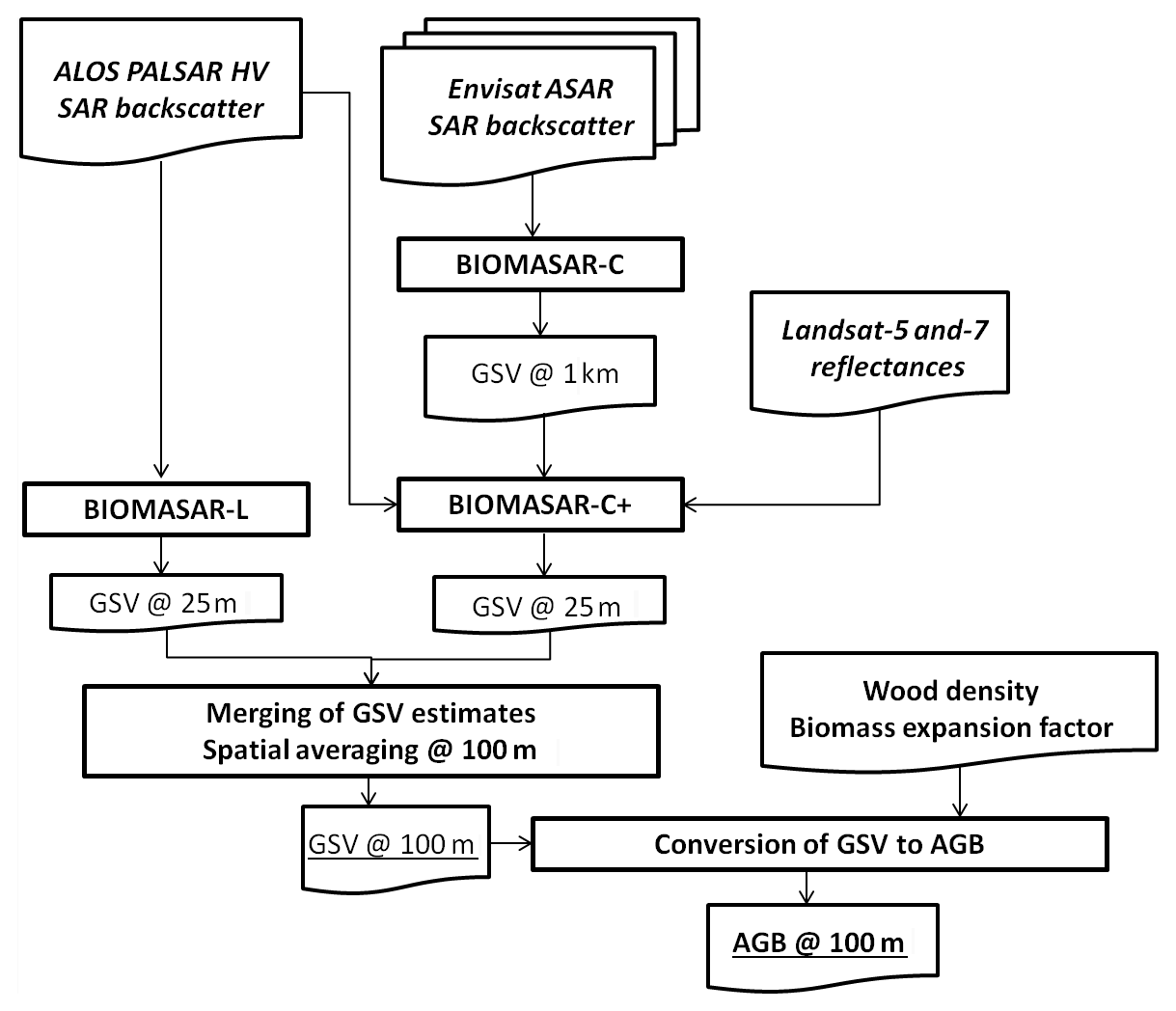
The AGB retrieval algorithm is outlined in the flowchart in Fig. 1 showing the interdependencies of datasets and retrieval models. We applied a model-based approach known as BIOMASAR (Santoro et al., 2011; Cartus et al., 2012b) separately to the ALOS PALSAR (Cartus et al., 2012b) and the Envisat ASAR radar backscatter datasets (Santoro et al., 2011, 2015a) to obtain two independent, spatially explicit estimates of GSV. BIOMASAR inverts the Water Cloud Model (Pulliainen et al., 1994; Santoro et al., 2002).

where ${\mathit{\sigma }}_{\text{for}}^{\mathrm{0}}$ represents the forest backscatter, i.e. the SAR backscatter observation from an ALOS PALSAR or an Envisat ASAR image (Sect. 2.1), and ${\mathit{\sigma }}_{\text{gr}}^{\mathrm{0}}$ and ${\mathit{\sigma }}_{\text{veg}}^{\mathrm{0}}$ represent the backscattering coefficients of the ground and vegetation layer, respectively. The exponential function, e^−βV, represents the two-way forest transmissivity, where β is an empirically defined coefficient expressed in m⁻¹, and V represents GSV. Equation (1) neglects multiple scattering, which is acceptable for most forest conditions (Santoro et al., 2011; Cartus et al., 2012a; Cartus and Santoro, 2019).

The model parameters β, ${\mathit{\sigma }}_{\text{gr}}^{\mathrm{0}}$, and ${\mathit{\sigma }}_{\text{veg}}^{\mathrm{0}}$ need to be estimated in order to invert the model and obtain an estimate of GSV from a measurement of the SAR backscatter. Estimates of the coefficient β are obtained with a model-based approach that relates canopy density and GSV observations through the transmissivity of the forest (Santoro et al., 2015a). The estimation is stratified by the FAO global ecological zones (Sect. S1, Fig. S2 and Table S2 in the Supplement). To estimate ${\mathit{\sigma }}_{\text{gr}}^{\mathrm{0}}$ and ${\mathit{\sigma }}_{\text{veg}}^{\mathrm{0}}$, we rely on a self-calibration approach (Santoro et al., 2011) rather than using a set of reference measurements of the SAR backscatter and in situ GSV values. The limited availability of in situ information on biomass (e.g. from inventory plots or laser-based maps) prevents adaptive calibration of retrieval algorithms using conventional approaches. In many areas, particularly the tropics, the number of available plots is very limited so that models can only be calibrated using reference information collected over large areas (Bouvet et al., 2018) with the risk of missing spatial variability in the backscatter. The model training approach is tailored to the radar wavelength in order to accommodate the different relationships of backscatter to biomass (BIOMASAR-C and BIOMASAR-L; see Sects. S2 and S3 in the Supplement).

When N observations of the radar backscatter are available, a final estimate of GSV, with higher accuracy compared to the individual estimates, is obtained by means of a weighted linear combination of the individual estimates of GSV obtained by inverting Eq. (1) for each backscatter observation (Santoro et al., 2011; Kurvonen et al., 1999).

In Eq. (2), the weights w_i are defined as the difference (${\mathit{\sigma }}_{\text{veg},i}^{\mathrm{0}}-{\mathit{\sigma }}_{\text{gr},i}^{\mathrm{0}}$) so that GSV estimates obtained from images with the strongest sensitivity to GSV are preferred to those obtained from images with no sensitivity to GSV (Santoro et al., 2011).

In this study, the BIOMASAR-C implementation was tailored to ingest ASAR data (Sect. S2 in the Supplement) and generated a GSV map at 1000 m spatial resolution by combining individual estimates from the ASAR dataset. The BIOMASAR-L implementation was tailored to ingest ALOS PALSAR data and generate a GSV data product at 25 m spatial resolution (Sect. S3 in the Supplement). The step in Eq. (2) became redundant because of the strong correlation of the ALOS PALSAR mosaics in time and the negligible weight attributed to the HH-polarized component when combined with the HV-polarized component. As a result, the retrieved GSV with BIOMASAR-L was based on the single observation of the L-band SAR backscatter at HV polarization in the mosaic for 2010.

To merge estimates of GSV obtained at 25 and 1000 m, the latter were rescaled to 25 m using a linear regression model (BIOMASAR-C+ in Fig. 1). The HH- and HV-polarized ALOS PALSAR backscatter (${\mathit{\sigma }}_{\text{HH}}^{\mathrm{0}}$ and ${\mathit{\sigma }}_{\text{HV}}^{\mathrm{0}}$) and the Landsat bands 3, 4, 5, and 7 (B₃, B₄, B₅, and B₇) were used as predictors in the model in Eq. (3):

The model was calibrated for each $\mathrm{1}{}^{\circ }\times \mathrm{1}{}^{\circ }$ tile at a pixel size of 1000 m to predict the BIOMASAR-C estimate of GSV at the 25 m scale. A bias correction had to be performed when retransforming the logarithmic GSV predictions to linear scale. The bias was computed by differencing the original BIOMASAR-C GSV and the predictions from Eq. (3) aggregated to the 1000 m pixel size. In spite of its simplicity, the multiple linear regression resulted in an overall superior performance when compared to results obtained with more sophisticated rescaling methods.

The final estimate of GSV was obtained by weighting the rescaled ASAR-based estimates (V_C+) and PALSAR-based estimates (V_L) of GSV. The weighting scheme accounted for the different sensitivity of C- and L-band data to GSV, the number of observations used for estimating GSV, local errors in the model training and inversion, and residual uncompensated topographic effects in the ALOS PALSAR mosaics (Sect. S4 in the Supplement). The GSV estimated with BIOMASAR-L was given more weight in areas of high GSV except in the case of steep terrain (Fig. S3 in the Supplement). BIOMASAR-C+ GSV estimates were instead preferred in areas of low GSV and regions with rugged terrain (Fig. S3 in the Supplement).

To reduce the pixel-wise variability due to speckle in the radar data and amplified by the weak sensitivity of the C- and L-band backscatter to forest variables, spatial averaging using a 4×4 window was applied. This decreased the spatial resolution of the GSV estimates to 0.000888^∘ in both latitude and longitude, corresponding to an area of approximately 1 ha at the Equator.

The conversion of GSV to AGB in Eq. (5) requires wood density (WD) and the biomass expansion factors (BEFs), which give the allometric relationship between stem mass and whole above-ground mass, including branches and leaves.

The spatial variations in WD and BEF result from biological processes that respond to local conditions, as has been demonstrated in regional studies showing environmental controls on the patterns of WD and BEF (Chave et al., 2009; Thurner et al., 2014). Towards a global assessment of WD patterns, we collected published databases based on inventory data where wood density (WD) is reported and explored machine learning methods to maximize the information content in relevant environmental variables (Sect. S5 in the Supplement). The final dataset of WD was obtained by integrating several individual predictions (Sect. S5 in the Supplement). To estimate the BEF, we used the generalized power-law function relating branch and leaf biomass to stem biomass (SB) (Thurner et al., 2014).

Because of the uneven distribution of samples for which biomass component measurements were available (Sect. S5 in the Supplement), the model in Eq. (6) was fitted to measurements of BEF and stem biomass for tropical and extra-tropical forests only, each stratified by leaf type (broadleaves, evergreen conifers, and deciduous conifers). All BEF models decreased rapidly for increasing stem biomass reaching an asymptote for low- to medium-stem biomass depending on ecoregion and leaf type. The asymptotic BEF for tropical broadleaf species was modelled with a value of 1.36, higher than other forest types, which were characterized by values of 1.15–1.20.

Spatially explicit estimates of WD and BEF were obtained at 0.01^∘ spatial resolution and resampled to the pixel size of the GSV dataset using bi-cubic interpolation. The AGB estimates resulting from the product of the GSV, WD, and BEF estimates were obtained at a spatial resolution of 0.000888^∘ in both latitude and longitude, i.e. with a pixel size of 1 ha at the Equator.

2.3 Uncertainty model

The uncertainty in the AGB estimates was quantified by their standard deviation. The standard deviation of the GSV estimates obtained with the BIOMASAR-C approach, δV_C, was quantified by propagating the standard deviation of the measured SAR backscatter, ${\mathit{\sigma }}_{\text{meas}}^{\mathrm{0}}$, and the estimates of the forest backscatter model parameters ${\mathit{\sigma }}_{\text{gr}}^{\mathrm{0}}$, ${\mathit{\sigma }}_{\text{df}}^{\mathrm{0}}$, β, and V_df (Santoro et al., 2015a).

The same approach was applied to the BIOMASAR-L procedure, in which case the error model also included components related to the average canopy density of dense forests, η_df; the average height of dense forests, h_df; and the two-way attenuation coefficient, α. Following the results in Simard et al. (2011) and Los et al. (2012), which validated GLAS-based height estimates at boreal, temperate, subtropical, and tropical forest sites, we assumed standard deviations for height estimates at the GLAS footprint-level between 4 m (boreal zone) and 10 m (tropical zone). As indicated by Garcia et al. (2012), the estimation error in canopy cover from ICESAT GLAS as the ratio of energy returned from the canopy to the total energy returned may be of the order of 15 to 20 %. We therefore assume a global error of 20 %. Differently than for the C-band case (Santoro et al., 2015a), the standard deviation of the coefficient β was inferred from the relationship of the forest transmissivity, simulated with the aid of GLAS height and optical canopy density estimates, and GSV. The 95 % bounds of the estimates increased from ±0.002 ha m⁻³ in the case of low values of β that are valid in boreal and subtropical dry forests to ±0.007 ha m⁻³ for the highest values of β that are applied in the tropics. For the two-way attenuation coefficient α, we assume a standard deviation of 0.25 dB m⁻¹, which is roughly consistent with the range of values reported in the literature.

In the case of BIOMASAR-C, the standard deviation of the multi-temporal GSV estimate was modelled as a linear combination of the single-image GSV standard deviations from Eq. (9) (Santoro et al., 2015a).

The uncertainty associated with the predictions of GSV obtained by rescaling the BIOMASAR-C GSV estimates was related to the uncertainty in the coarse-resolution GSV estimates and the scaling factors.

The relative standard deviation of the BIOMASAR-C GSV estimates ($\mathit{\delta }{V}_{\text{C}}/V_c$) was modelled as a function of the GSV estimates (V_C) by means of an exponential model. In Eq. (10), the model coefficients a, b, and c were estimated by means of a least squares regression for each of the FAO global ecological zones.

To characterize the error associated with the rescaling model, we used the root mean square difference (RMSD) between the original BIOMASAR-C GSV and the BIOMASAR-C+ GSV estimates aggregated to the pixel size of the former. A polynomial function of the fourth order was found to adequately reproduce the relationship between the GSV sets across ecozones and was used to fit the observed trend in GSV.

In the process of rescaling, we assumed that the standard deviation scaled with the pixel area of the GSV predictions. In Eq. (11), the scaling factor between standard deviations was represented by the ratio between the pixel areas of the rescaled product (A_c+) and the BIOMASAR-C data product (A_c):

The standard deviation of the GSV estimates was obtained with the same weighted linear combination of the standard deviations of the BIOMASAR-L and the BIOMASAR-C+ datasets:

The standard deviation of AGB was expressed in terms of partial derivatives of its components:

The standard deviation of the wood density estimates, δWD, was obtained by computing the variance of the predictions for each measurement of wood density and fitting a linear model (Fig. S4 in the Supplement). The standard deviation of the BEF was expressed in terms of partial derivatives of its components:

In Eq. (14), δp₁ and δp₂ represent the standard deviations of the two coefficients of the BEF model.

2.4 Validation

To assess the accuracy of the AGB estimates, we used a reference dataset of AGB observations from 110 897 forest field inventory plots. The data were gathered from a variety of surveys undertaken by national forest inventories and research networks (Sect. S6 in the Supplement).

The opportunistic nature of our validation database led to an uneven spatial distribution of the reference samples (Fig. S5 in the Supplement) as well as a variety of plot sizes, survey methods, and allometric equations used (Tables S3 and S4 in the Supplement). The plots were mostly smaller than 1 ha (Table S3 in the Supplement), implying that they often represented a small fraction of the area covered by a 1 ha map pixel. To reduce the effect of random errors caused by the mismatch in resolution between the reference dataset and our map model, we aggregated our map and the plot data to 0.1^∘ grid cells. This represented a trade-off between capturing the local-scale variability in AGB whilst allowing a number of plot measurements deemed sufficient to compute an average AGB representative of the area within the grid cell. In the end, our assessment cannot provide an indication of the validity of pixel-based AGB estimates. Instead, it provides a measure of the accuracy of generalized spatial AGB patterns. This is, however, a pragmatic approach when using measurements not designed for validation of estimates from remote sensing imagery but which often provide the only source of information on AGB in poorly inventoried regions or regions where national inventory data are not publicly available.

To provide a more comprehensive overview of the reliability of the spatial patterns in areas not covered by the database of plot inventory measurements, the analysis was supplemented by a comparison of average GSV or AGB at the level of inventory reference units (polygons, counties, provinces, and ecoregions). The scope of this analysis was primarily to identify systematic errors, on a large scale, that may not become evident when comparing at the individual plot level. For a quantitative assessment of the retrieval at the scale of provincial and regional aggregates, we computed the RMSD between map and reference biomass averages relative to the average reference biomass and the bias between map and reference biomass averages. The RMSD was computed as a weighted mean of the errors, where the weights corresponded to the ratio of the forest area to the total forest area. For Russia (Sect. S6 in the Supplement), GSV and AGB data were gathered for approximately 1600 forest managements units (FMUs) ranging in size from 3000 ha (e.g. intensive forestry or national parks in the European part) to 30 000 000 ha (remote territories in Siberia). For countries with a well-established national forest inventory that regularly publish regional statistics of forest biomass at the level of administrative or ecological units, we assembled a database of GSV and AGB averages representative of the epoch 2010 (Sect. S6 in the Supplement).

2.5 Inter-comparison of AGB maps

The spatial distribution of AGB map estimates from our dataset was compared with biome and global forest AGB maps based on satellite remote sensing observations (Saatchi et al., 2011b; Baccini et al., 2012; Thurner et al., 2014; Liu et al., 2015; Avitabile et al., 2016; Santoro et al., 2015a) or ancillary datasets (Kindermann et al., 2008). While an additional assessment of our dataset against regional maps of AGB would further contribute to building confidence in the data product, it is felt that such investigations require their own framework also making use of local reference data and expert knowledge, as for example undertaken for Europe (Avitabile and Camia, 2018), the US (Spawn et al., 2020), and Tanzania (Næsset et al., 2020).

To do this, the datasets were first harmonized to a common geographic map projection and resampled to a pixel size of 0.01^∘. Datasets expressing AGB in carbon units (Mg C ha⁻¹) were converted to AGB using a carbon fraction default value of 0.47 (IPCC, 2006) (Table S5 in the Supplement). All datasets span a decade of input observations from 2000 to 2010 but could not be harmonized to reflect the conditions of a single epoch due to the lack of information on growth rates. This, however, is not expected to have significant effects on the interpretation of the latitudinal profiles.

As a way of assessing the AGB patterns of each map, we compared latitudinal averages based on values from the 0.1^∘ validation grid cells with corresponding values from the database of forest inventory plots. To obtain a homogeneous representation of all latitudes, we grouped grid cells in 10^∘ wide intervals.

3.1 Global AGB dataset

The global AGB dataset (Fig. 2) was obtained by scaling global estimates of GSV (Fig. S6 in the Supplement) using model-based estimates of wood density (Fig. S7 in the Supplement) and stem-to-total biomass expansion factors (Fig. S8 in the Supplement). The uncertainty in the AGB estimates is reported as standard deviation (Fig. 2). The models for retrieving GSV and converting it to AGB were developed for woody vegetation, so we evaluated the estimates corresponding just to forest cover by regrouping the classes from the Climate Change Initiative Land Cover (CCI-LC) dataset of 2010 into forest and non-forest land (Sect. S1, Table S7 in the Supplement).

At the 1 ha scale, the largest predicted value was 757 Mg ha⁻¹, corresponding to a GSV of 1087 m³ ha⁻¹, in forests of the US Pacific Northwest. However, for 99 % of the world's forests, AGB was estimated to be less than 360 Mg ha⁻¹, and 90 % was below 182 Mg ha⁻¹, which explains truncating the colour bar in Fig. 2 at 500 Mg ha⁻¹. The spatial distribution of AGB followed a clear latitudinal gradient (Fig. 2). In the Northern Hemisphere, AGB increased steadily with decreasing latitude across the boreal zone (between 75 and 60^∘ N), then remained fairly constant throughout the temperate (between 60 and 40^∘ N) and subtropical (between 40 and 20^∘ N) zones. AGB increased sharply as we enter and leave the tropical zone between 20^∘ N and 20^∘ S, though with a minimum at 13^∘ N due to the large area of low-biomass dry forests in the sub-Sahelian region. The AGB of semi-tropical forests in the Southern Hemisphere between 20 and 33^∘ S was slightly lower than in the corresponding latitude range in the Northern Hemisphere because of the larger proportion of low-density forest. The local maximum at 25^∘ S corresponded to the Atlantic forests of Brazil and dense subtropical forests along the east coast of Australia, where biomass accumulation is favoured by higher precipitation. Temperate forests had higher AGB in the Southern Hemisphere (south of 33^∘ S) than in the Northern Hemisphere because of the predominant highly productive evergreen and coniferous forest along the Chilean–Argentinean Andes, in south-eastern Australia, and New Zealand. The peak at 42^∘ S corresponds to the broadleaved forests of Tasmania.

The AGB standard deviation, expressed in Fig. 2 relative to the AGB estimates, was on average 50 % with an inter-quartile range of values between 44 % and 61 %. The rather constant relative uncertainty is also illustrated by the horizontal bars in the latitudinal profile of Fig. 2, which scale with the AGB level. The relative standard deviation was smaller than 100 % for approximately 95 % of the mapped pixels, which explains truncating the colour bar of the AGB standard deviation map in Fig. 2 at 100 %. The large majority of the AGB estimates for which the standard deviation exceeded the 100 % level were below 20 Mg ha⁻¹, such as in sparsely vegetated regions corresponding to the transition to tundra in Canada and Alaska, the Siberian Lowlands and Far East Russia, or in poorly stocked forests such as in northern China and western Madagascar.

The small-scale variability in AGB in forest landscapes is captured by the 1 ha pixel spacing of the dataset (Figs. 3 and 4). The example in Fig. 3 shows the region of the Bratsk Reservoir formed by the Angara River in central Siberia, where forests are heavily managed for timber production. Clear-felling activities occur in polygons often larger than 10 ha. The map for a $\mathrm{1}{}^{\circ }\times \mathrm{1}{}^{\circ }$ area east of the reservoir shows forests with AGB above 100 Mg ha⁻¹, roughly corresponding to a GSV of at least 200 m³ ha⁻¹, interspersed with small rectangular white shapes corresponding to clear-cut areas (Fig. 3). Our estimates give more detailed information on the spatial patterns of AGB in this region than the AGB product by Thurner et al. (2014) based on remote sensing data with a spatial resolution of 1000 m.

The example in Fig. 4 includes part of Trans-Amazonian Highway south of the Amazon River in the state of Pará, Brazil. This region is characterized by fish bone deforestation caused by lateral expansion of agriculture from the highway into pristine forest. The fish bone pattern is clear in our AGB map (Fig. 4, top left panel), and some isolated, small-scale patches of deforestation are also visible. For comparison, Fig. 4 shows AGB estimates by three pan-tropical maps based on remote sensing observations (Saatchi et al., 2011b; Baccini et al., 2012; Avitabile et al., 2016). Because it was based on satellite data acquired around the year 2000, the deforestation patterns are less extended in the map by Saatchi et al. (2011b) compared to the maps by Baccini et al. (2012), based on observations taken in 2007, and Avitabile et al. (2016), which merged the other two pan-tropical datasets. The level of detail in our map is much greater because of the 1 ha spatial resolution compared to 25 ha in Baccini et al. (2012) and nearly 100 ha in Avitabile et al. (2016) and Saatchi et al. (2011a)

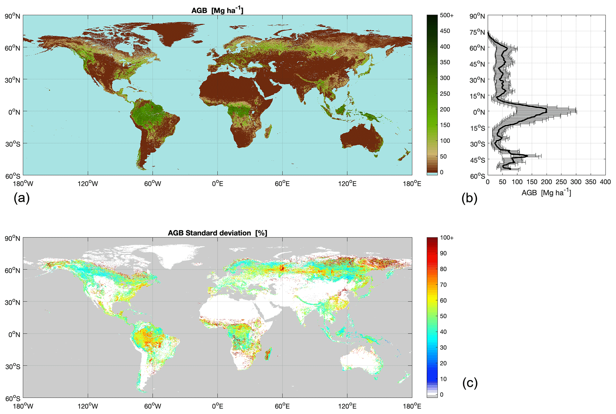
Figure 2Map estimates of AGB (a) and AGB standard deviation expressed relative to the AGB (b). The colour bar of the AGB map has been truncated at 500 Mg ha⁻¹ to increase contrast. Similarly, the colour bar of the AGB relative standard deviation has been truncated at 100 %. The right-hand panel shows the profile of average AGB along latitude (thick solid line) and the two-sided average standard deviation of AGB at a given latitude (horizontal bars).

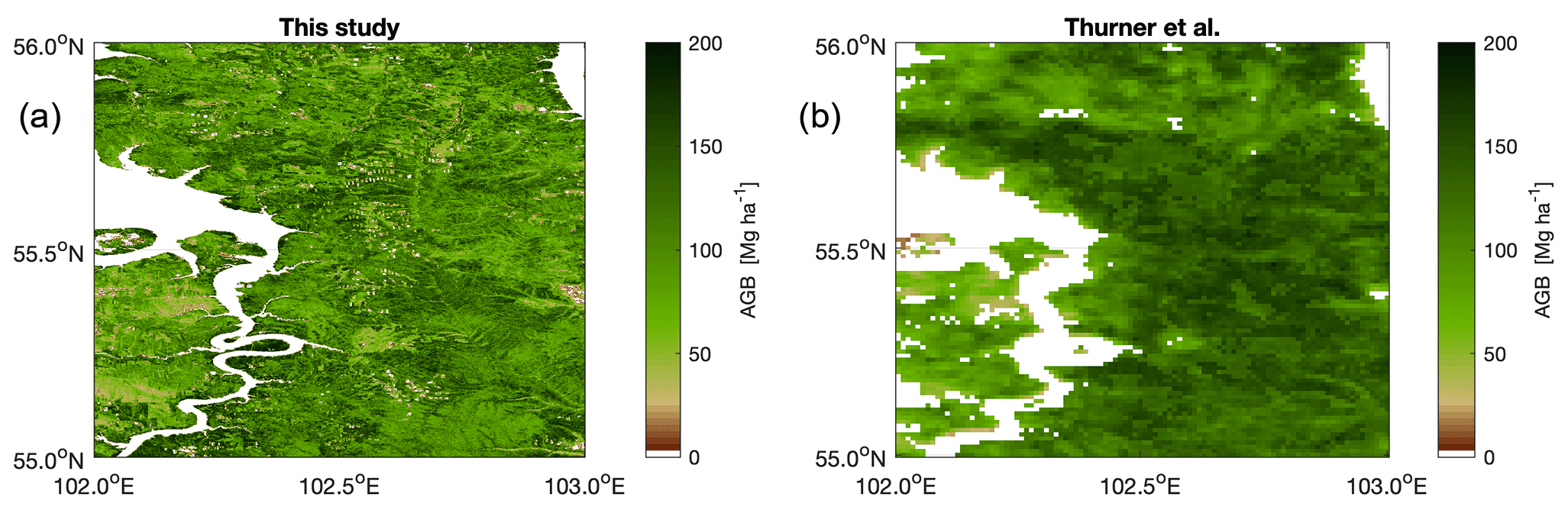
Figure 3AGB estimates from this study (left) and from Thurner et al. (2014) for a $\mathrm{1}{}^{\circ }\times \mathrm{1}{}^{\circ }$ area in central Siberia.

Figure 4AGB estimates by this study (a), Avitabile et al. (2016) (b), Saatchi et al. (2011b) (c), and Baccini et al. (2012) (d) for a $\mathrm{1}{}^{\circ }\times \mathrm{1}{}^{\circ }$ area in the state of Parà, Brazil.

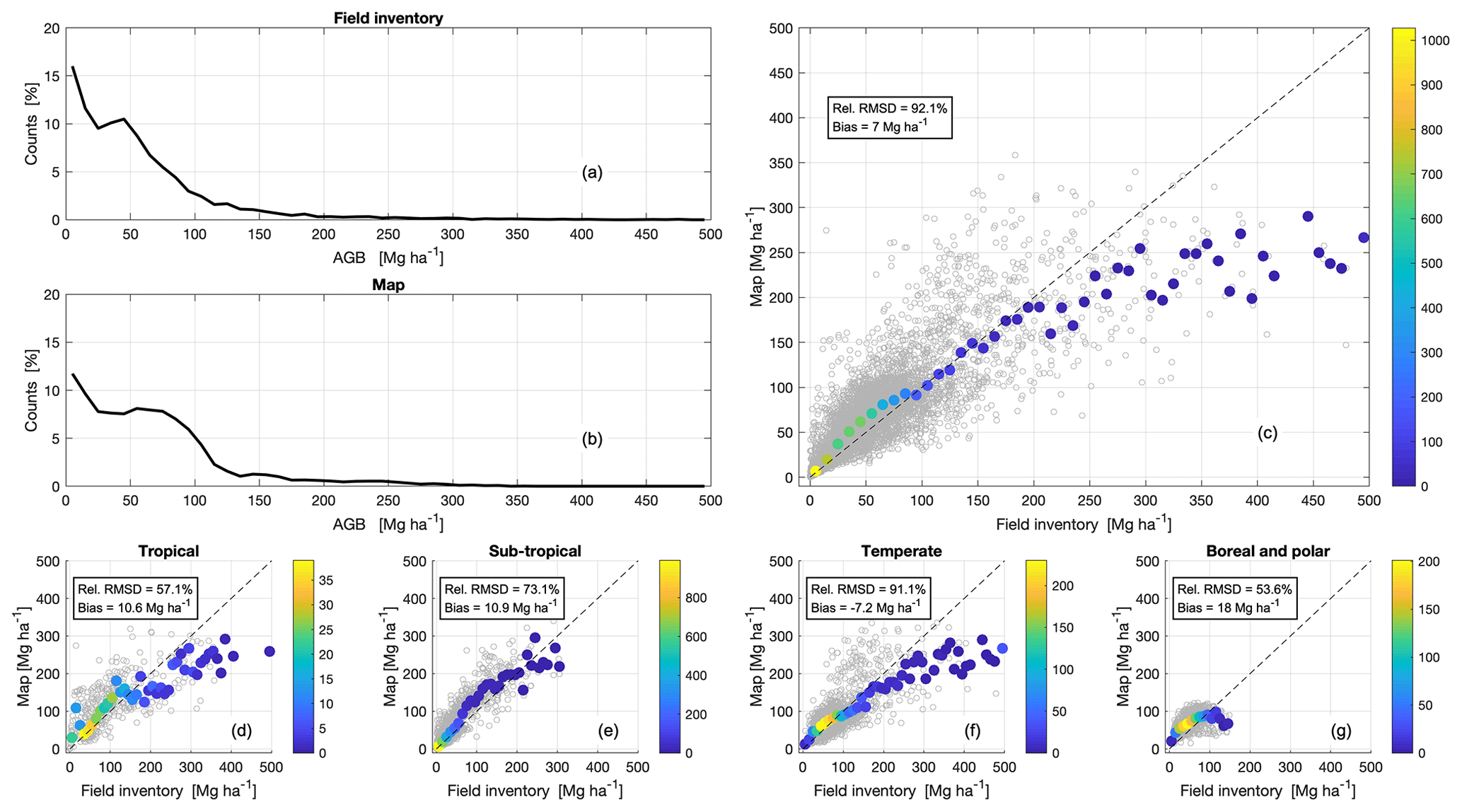
Figure 5Histograms of AGB from the field inventory database (a) and the map (b) for 0.1^∘ grid cell values. (c) Scatterplot of map AGB against field inventory values for 0.1^∘ grid cells (grey circles); the filled circles show the median AGB of the map values in each 10 Mg ha⁻¹ wide interval of field inventory AGB values. The colour bar represents the number of grid cells within a given AGB interval. Similar scatterplots are given for the tropical zone (d), the subtropical zone (e), the temperate zone (f), and the boreal and polar zones (g) according to the FAO global ecological zones. On each scatterplot, we report the root mean square difference (RMSD) between map and field inventory AGB relative to the mean value of the reference AGB and the bias, i.e. the difference between mean values of the map AGB and the reference AGB. To improve presentation and because of the paucity of grid cells with AGB above 500 Mg ha⁻¹, axes are truncated at 500 Mg ha⁻¹.

Download

Table 1Total AGB, forest area, and average AGB per major ecozone.

Download Print Version | Download XLSX

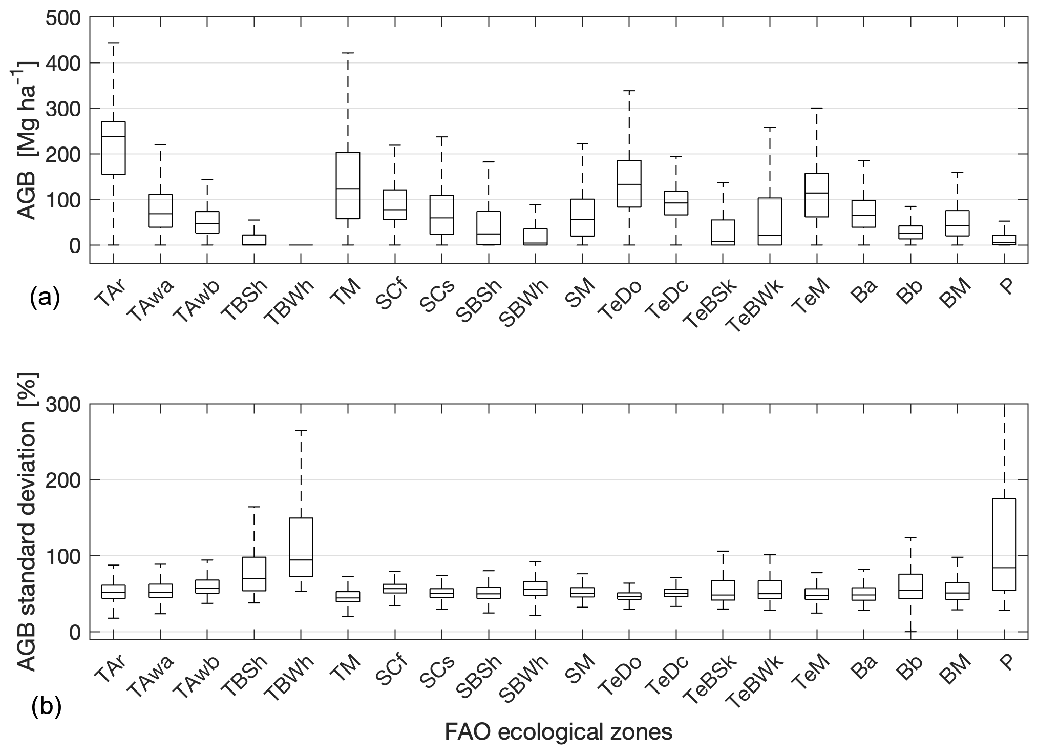
Figure 6Box plot diagram of AGB (a) and its standard deviation by FAO global ecological zone. On each box, the central mark indicates the median, the bottom and top edges delimit the interquartile range, and the whisker delimits the 1–99 percentile range. Labels of global ecological zones: TAr – tropical rain forest, TAwa – tropical moist deciduous forest, TAwb – tropical dry forest, TBSh – tropical shrubland, TBWh – tropical desert, TM – tropical mountain systems, SCf – subtropical humid forest, SCs – subtropical dry forest, SBSh – subtropical steppe, SBWh – subtropical desert, SM – subtropical mountain systems, TeDo – temperate oceanic forest, TeDc – temperate continental forest, TeBSk – temperate steppe, TeBWk – temperate desert, TeM – temperate mountain systems, Ba – boreal coniferous forest, Bb – boreal tundra woodland, BM – boreal mountain systems, P – polar.

Download

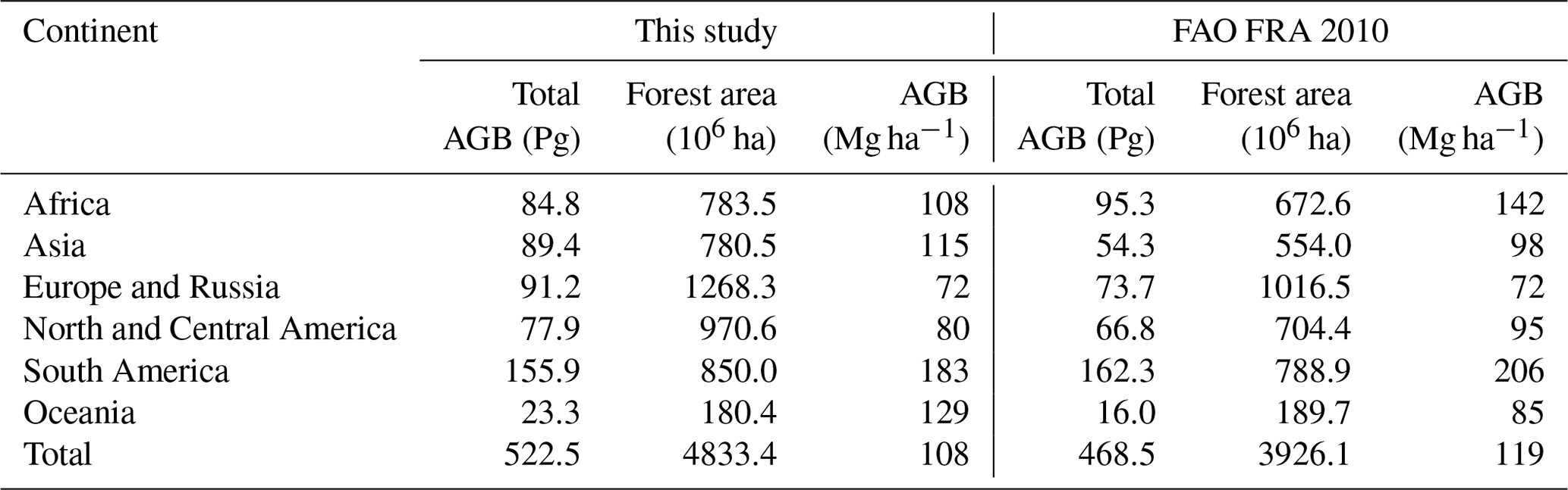
Table 2Total AGB (unit: Pg), forest area (unit: ha), and average AGB (unit: Mg ha⁻¹) per continent from this study and from the FAO FRA 2010. The forest area column for the FRA does not account for countries reporting forest area but not AGB. For Asia, North and Central America, and South America, 5 %, 1 %, and 10 % of the forest area did not contribute to the AGB to the FRA. For Africa, Europe and Russia, and Oceania, less than 1 % of the forest area did not contribute to the FRA. The total forest area from the FRA is 4.033×10⁶ ha.

Download Print Version | Download XLSX

3.2 Validity of AGB estimates

AGB averages were obtained for 6456 0.1^∘ grid cells including at least five inventory plots (Sect. S6 in the Supplement). These grid cells represented approximately 1 % of the Earth's forest cover. The grid cell average AGB from the field inventory database ranged from 0 to 1670 Mg ha⁻¹ (median: 43 Mg ha⁻¹; mean: 60 Mg ha⁻¹; 99th percentile: 351 Mg ha⁻¹). The AGB histogram was skewed towards low values (Fig. 5a) because of the large proportion of measurements from the National Forest Inventories of Spain and Sweden (Table S4 in the Supplement). The grid cell average AGB from the map ranged from 0 to 358 Mg ha⁻¹ (median: 57 Mg ha⁻¹; mean: 67 Mg ha⁻¹; 99th percentile: 278 Mg ha⁻¹). The AGB histograms from the map (Fig. 5b) and the field inventory (Fig. 5a) were similar, with a mode at around 0, a decline to a shoulder, then a further decline to a long tail. In the field inventory the shoulder covered the range 25–50 Mg ha⁻¹ and was followed by a slow decline, but for the map it extended to around 80 Mg ha⁻¹ and then declined rapidly. This difference arises because the map tends to give higher values than inventory in the lower AGB range (Fig. 5c and Fig. S9 in the Supplement). These trends have been reported for other pan-tropical and regional AGB studies (Avitabile et al., 2016; Rodríguez-Veiga et al., 2019). The scatterplot of map against inventory values of AGB in Fig. 5c and the RMSD curve in Fig. S9 in the Supplement indicate an agreement in trend between field inventory and map values up to about 250 Mg ha⁻¹. Above 250 Mg ha⁻¹, the map values rose as the field inventory value did, albeit more gently and with much greater variance. Disaggregating the data by major ecological domains, using the FAO global ecological zones as reference, suggested slight differences in the agreement between map and inventory values in tropical, subtropical, and temperate forests (Fig. 5d–f).

3.3 Spatial distribution of AGB

Combining our AGB dataset with the CCI Land Cover dataset and the FAO ecological zones, we estimated a total AGB of 521 Pg for a forest area of 4825 million ha, corresponding to a global average forest AGB of 108 Mg ha⁻¹ (Table 1). Using the carbon fraction default value of 0.47 (IPCC, 2006), we estimated a total above-ground carbon stock of 246 Pg C. Tropical forests had the highest average AGB (147 Mg ha⁻¹), representing 64 % of the total forest AGB and 47 % of the total forest area. The second-largest average AGB was found in temperate forests (102 Mg ha⁻¹), which accounted for 14 % of the total AGB and 15 % of the total forest area. Subtropical and boreal forests had similar average AGB (75 and 60 Mg ha⁻¹, respectively), but the area covered by the latter was almost 3 times larger. As a result, the total AGB of boreal forests was more than twice as large as that of subtropical forests and corresponded to 16 % of the total AGB, thus being larger than the AGB pool in temperate forests. The total AGB of subtropical forests accounted for 7 % of the global AGB. The contribution of polar forests to the global AGB pool was negligible (0.1 %).

Looking at Fig. 6, the tropical rainforest (TAr) ecozone hosted primarily high-density forests, with a median AGB of 238 Mg ha⁻¹ and the low end of the interquartile range above 150 Mg ha⁻¹. Besides tropical rainforests, only the tropical mountain, temperate oceanic, and temperate mountain ecozones (TM, TeDo, and TeM, respectively) had median AGB values above 100 Mg ha⁻¹ (Fig. 6). For the tropical, subtropical, and temperate ecozones, the AGB of forests in dry environments (shrubland, steppe, and desert) was lower than in wet environments (rainforest, moist, humid, mountain, continental, and oceanic). The AGB of boreal forests decreased with increasing latitude from the boreal coniferous (Ba) ecozone located at the southernmost edge of the boreal ecotone, through the boreal mountain (BM) ecozone, to the boreal tundra woodland (Bb) ecozone at the northernmost edge of the boreal zone.

The AGB standard deviation relative to the AGB estimates was fairly constant across most ecological zones (Fig. 6). The median value ranged between 44 % and 57 %, except for the tropical shrubland, tropical desert, and polar ecozones (TBSh: 69 %; TBWh: 92 %; and P: 84 %). The largest proportion of the AGB standard deviation was attributed to the uncertainty in the GSV estimates (Fig. S10 in the Supplement). The uncertainty in the wood density estimates accounted for 7 % to 20 % (mean: 14 %) of the AGB standard deviation (Fig. S10 in the Supplement), while the uncertainty in the BEF accounted for between 2 % to 13 % of the AGB standard deviation (mean: 7 %) with the exception of the tropical desert zone (30 %) (Fig. S10 in the Supplement). The uncertainty in the GSV was driven by the weak sensitivity of the radar backscatter to increasing GSV, an effect further exacerbated in wet environments (Santoro et al., 2015a), thus explaining the slightly higher uncertainty in the tropics and the subtropics. The larger uncertainty in sparsely forested regions compared to densely forested regions (Fig. 2) is a consequence of the substantially larger uncertainty in the ${\mathit{\sigma }}_{\text{gr}}^{\mathrm{0}}$ parameter compared to the uncertainty in the ${\mathit{\sigma }}_{\text{veg}}^{\mathrm{0}}$ in the GSV retrieval model in Eq. (1) (Fig. S11 in the Supplement). In sparse forests or forests with low woody biomass stocks, the total backscatter from the forest is dominated by the ground scattering component, i.e. the term with ${\mathit{\sigma }}_{\text{gr}}^{\mathrm{0}}$ in Eq. (1), thus being affected by larger uncertainty compared to the backscatter received from dense forests, for which the largest contribution to the measured backscatter is attributed to the scattering from the canopy, i.e. to the term with ${\mathit{\sigma }}_{\text{veg}}^{\mathrm{0}}$ in Eq. (1).

3.4 Assessment of global forest biomass resources

The most comprehensive summary of global forest resources and biomass pools is reported by the FAO in their quinquennial FRA. For the FRA, each country reports its values of forest area (in hectares), total AGB (in petagrams), and average AGB (in Mg ha⁻¹) according to their inventory capabilities. Forest area was derived from inventory data or remote sensing data. AGB statistics were derived either from measurements collected as part of national inventories, local inventories, or estimates reported in the literature. Adjustments were applied by the FAO where necessary to ensure consistency with its own information sources on forest area and biomass resources. While all 233 countries contributing to the FRA for 2010 reported their estimates of forest area, only 171 reported total AGB and average AGB. Of the remaining 62 countries, accounting for approximately 2.6 % of the global land surface, 10 reported no forest cover, while 7 (Fiji, Eritrea, Uruguay, Ecuador, Paraguay, Japan, and Venezuela) reported an estimate of forest area exceeding 10⁶ ha. Of the countries reporting on AGB, 111 derived their average AGB from values of the average GSV using one or multiple biomass conversion and expansion factor (BCEF) values. This was common practice for countries lacking a systematic national forest inventory. Among these, 79 relied on default numbers published by the Intergovernmental Panel on Climate Change (IPCC) (IPCC, 2006) (Table S7 in the Supplement).

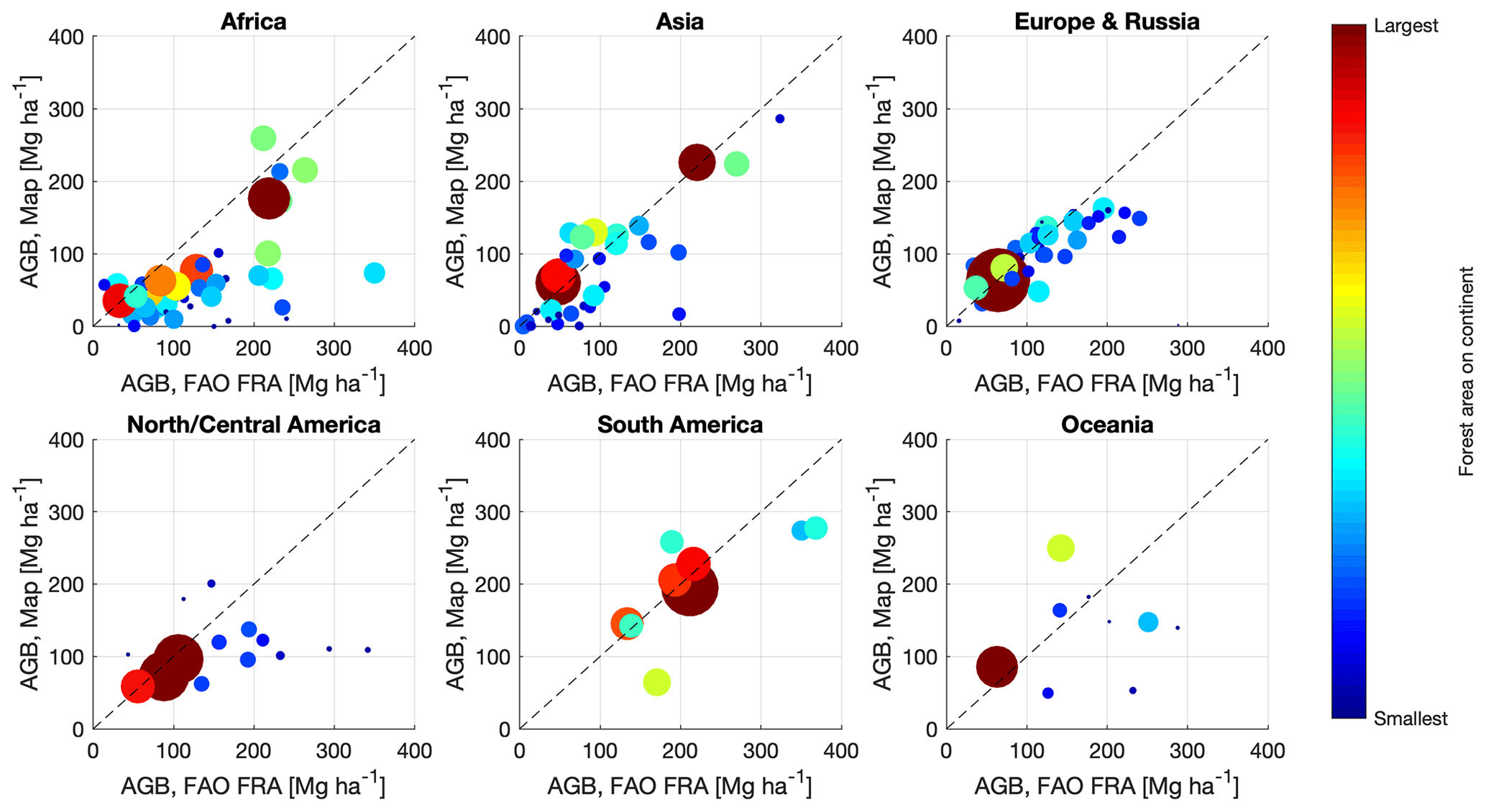
Figure 7Average AGB per country from the FAO FRA 2010 country reports and our map dataset. Countries have been grouped per continent. The size of each circle is proportional to the forest area of the country derived from the CCI Land Cover dataset (same scaling across all continents). The colour ramp associated with the circles gives a graphical representation of the relative country forest area (different for each continent).

Download

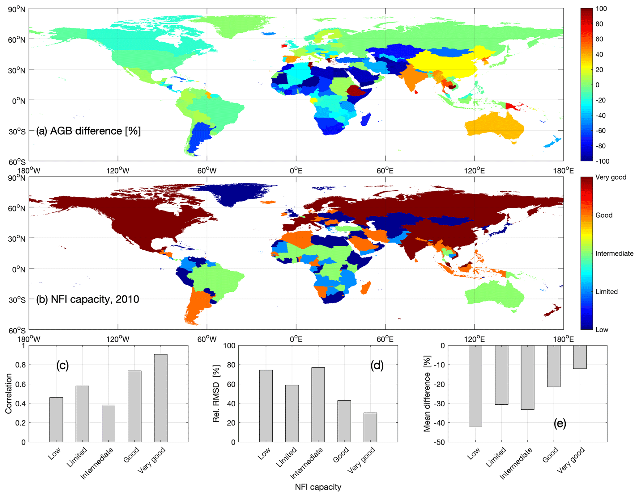
Figure 8Difference between country AGB from our map and FRA (expressed relative to the FRA AGB) (a), NFI capacities for the year 2010 (Romijn et al., 2015) (b), Pearson's correlation coefficient (c), relative RMSD (d), and mean difference between map estimates of country AGB and values from the FRA for NFI capacity level (e). Number of countries per NFI capacity level: 51 (low), 30 (limited), 26 (intermediate), 37 (good), and 23 (very good).

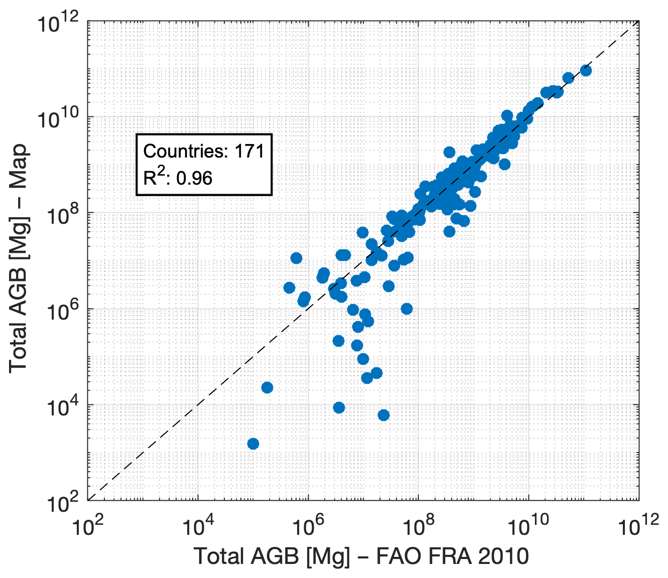
Figure 9Total AGB from the FAO FRA 2010 country reports and from our dataset (see Table S7 in the Supplement for details).

Download

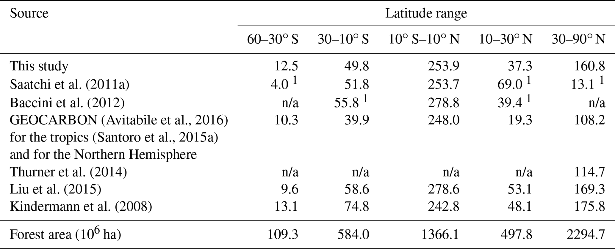
Table 3Total AGB (Pg) for five latitude ranges roughly corresponding to the temperate forests of the Southern Hemisphere (60–30^∘ S), the humid and dry tropics of the Southern Hemisphere (30–10^∘ S), the wet tropics (10^∘ S–10^∘ N), the humid and dry tropics of the Northern Hemisphere (10–30^∘ N), and the temperate and boreal forests of the Northern Hemisphere (30 and 90^∘ N). Values marked with superscript 1 indicate partial coverage of the latitude range by the corresponding map; n/a indicates not available in the latitude range. The forest area for each range is reported on the last line.

Download Print Version | Download XLSX

3.4.1 Global and continental statistics

The statistics on forest area, average AGB, and total AGB from the FRA 2010 and from the combination of our AGB dataset with the CCI Land Cover dataset are reported by continent (Table 2). Our total AGB estimate of 522 Pg was 11 % higher than the value of 468 Pg reported by the FRA. This difference is a consequence of the 23 % larger forest area estimated from the CCI Land Cover dataset (Table 2) despite the FRA reporting 9 % higher global average AGB than our estimate (119 vs. 108 Mg ha⁻¹; Table 2). Compared to Table 1, based on the FAO global ecological zones dataset to delineate land surfaces, we estimate an additional 8×10⁶ ha of forest area and an additional 1.5 Pg of total AGB as a consequence of the more precise delineation of the land surface by the Database of Global Administrative Areas used as reference for the countries' boundaries (GADM, http://www.gadm.org, last access: 9 August 2021).

For the three continents spanning the tropics, we found the highest average AGB in South America, although our estimate (183 Mg ha⁻¹) was 11 % lower than the corresponding value from the FRA (206 Mg ha⁻¹) (Table 2). South America also contained the largest total AGB pool. Although our estimate (155.9 Pg) was only 4 % smaller than the FRA (162.3 Pg), the FRA did not provide AGB for approximately 10 % of the forest area of South America (Table 2). We found a larger difference between our results and those of FAO for Africa. The average AGB from our dataset was 24 % lower than the FRA (108 Mg ha⁻¹ vs. 142 Mg ha⁻¹; Table 2), whilst the total AGB was only 11 % smaller than in the FRA (84.8 vs. 95.3 Pg) due to the larger forest area we used from the CCI Land Cover dataset. In contrast, for Asia the average AGB from our dataset (115 Mg ha⁻¹) was 17 % higher than in the FRA (98 Mg ha⁻¹) (Table 2), while our estimate of total AGB exceeded that from the FRA by 64 % (89.4 vs. 54.3 Pg) mainly because of the 40 % larger forest area estimated from the CCI Land Cover dataset.

For the two continents spanning the northern boreal and temperate zones, the average AGB values from our estimates were well below 100 Mg ha⁻¹ (Table 2). The average AGB estimate for Europe differed by less than 1 % (Table 2) compared to the FRA, whereas for North and Central America the difference was 15 %. Because the forest area estimated from the CCI Land Cover dataset was larger than the FRA values, the total AGB estimated from our dataset was larger than the values reported in the FRA by 20 % for Europe and 14 % for North and Central America.

Finally, the smallest of the continental pools of AGB was in Oceania, where our larger estimate of total AGB compared to the FRA was primarily explained by our estimate of AGB being on average almost 35 % larger than the value derived from the FRA.

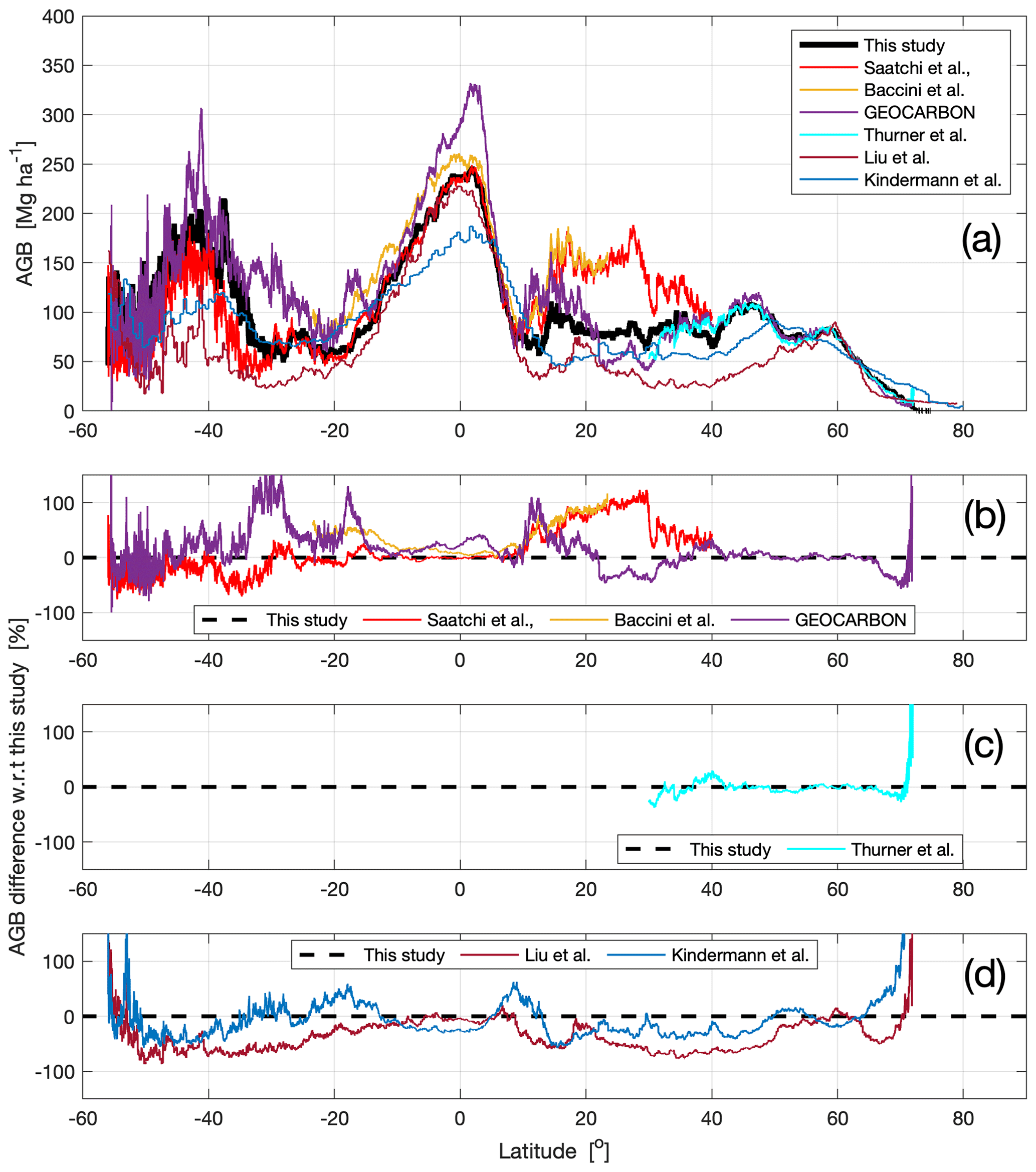
Figure 10Profiles of average AGB along latitude for each dataset listed in Table 3 (a), together with the corresponding relative difference between the latitudinal AGB derived from the other datasets and this study (b–d), expressed in percentage values relative to our estimates.

Download

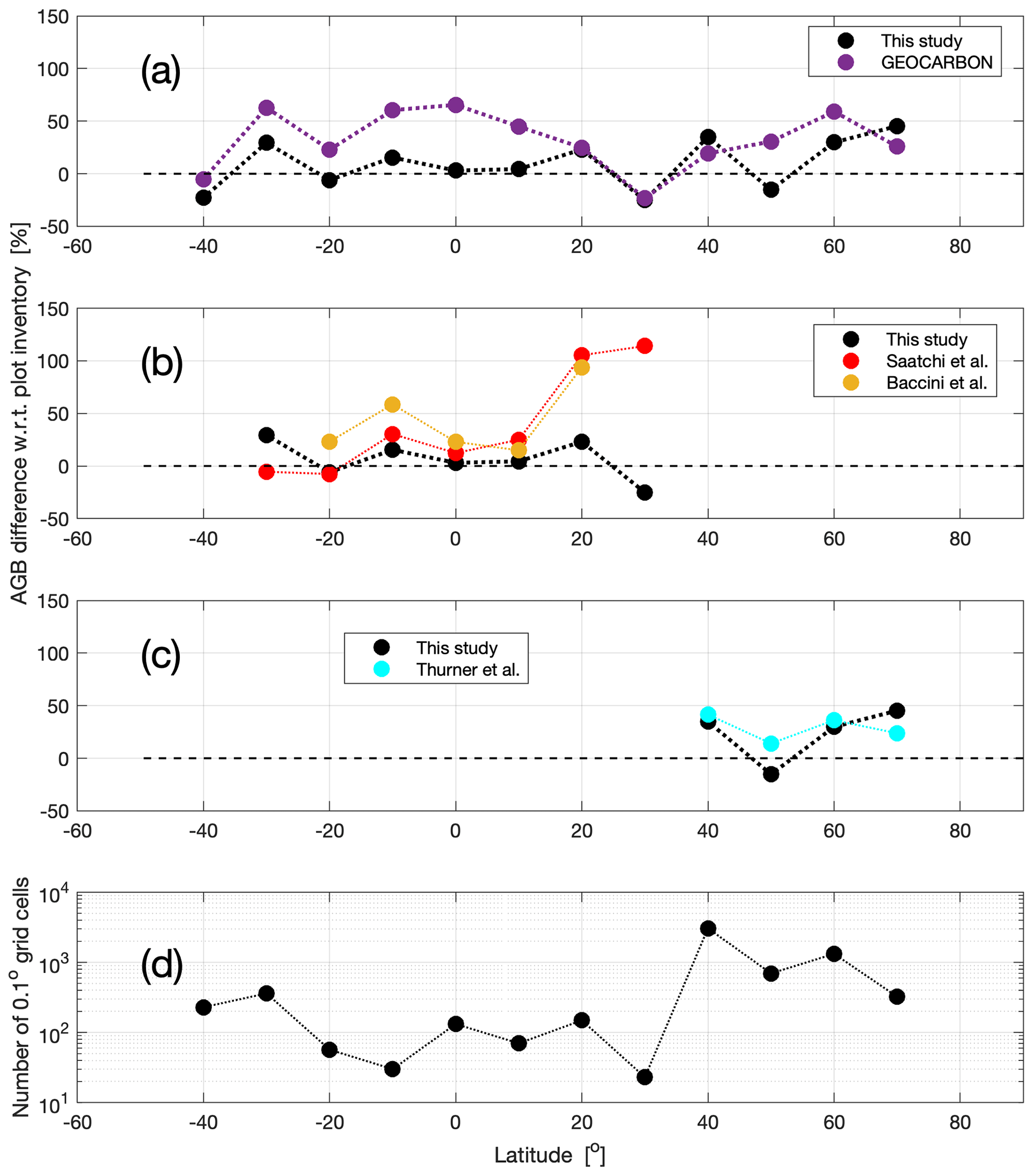
Figure 11Relative difference in AGB from maps and plot inventory data averaged over the 0.1^∘ grid cell validation cells (a–c). The number of grid cells stratified by 10^∘ wide latitude intervals is illustrated in (d).

Download

3.5 Comparison of map estimates of AGB

All map datasets analysed in this study including ours (Table 3) showed similar latitudinal trends (Fig. 10a), with the highest AGB in the Southern Hemisphere at 40^∘ S and across the Equator and low AGB in the dry tropics at around 20^∘ S and north of 10^∘ N. However, there were some large differences between the maps (Fig. 10a), illustrating the current uncertainty about the global forest carbon pools.

For the wet tropics between 15^∘ S and 10^∘ N, the AGB from our dataset was close to that from the pan-tropical dataset by Saatchi et al. (2011a) (Fig. 10b) but is between 10 % and 50 % lower than the values by Baccini et al. (2012), and the GEOCARBON dataset. The analysis of the latitudinal averages based on the 0.1^∘ grid cell AGB values show an overestimate of AGB in these two datasets by about 10 % to 60 %. In contrast, the average AGB values from our dataset were only higher than the corresponding values from the plot inventory database by a few per cent (Fig. 11a and b).

The differences between our dataset and each of the pan-tropical AGB datasets were much larger in tropical and subtropical regions north and south of the wet tropics. In the Northern Hemisphere, between 10 and 30^∘ N, Saatchi et al. and Baccini et al. (2011a, 2012) exceeded our estimates by between 40 % and 110 % (Fig. 9b). For the same latitude range, the GEOCARBON dataset differed from our values by 110 % to −47 % with increasing latitude (Fig. 10b). The latitudinal averages at the 0.1^∘ grid cells confirmed that all three maps were strongly biased, while our dataset was closer to the values obtained from the plot inventory dataset (Fig. 11). The GEOCARBON dataset presented both positive and negative biases, being about 50 % of the average AGB from the plot inventory dataset (Fig. 11a). The overestimate exceeded 100 % of the average AGB from the plot inventory dataset in the case of Saatchi et al. and Baccini et al. (2011a, 2012) (Fig. 11b). In the Southern Hemisphere, between 35 and 15^∘ S, the GEOCARBON dataset and Baccini et al. (2012) exceeded our AGB by 20 % to 160 %, whereas Saatchi et al. (2011a) differed from our values by between +20 % and −60 % (Fig. 10b). The comparison at the level of the 0.1^∘ grid cells indicates an overestimate by GEOCARBON and Baccini et al. (2012) between 20 % and 60 % of the average AGB from the plot inventory data (Fig. 11a and b, respectively). The difference between the average AGB from our dataset and from Saatchi et al. (2011a) with respect to values from the plot inventory dataset were instead mostly below 20 %.

For the Southern Hemisphere temperate forests south of 35^∘ S, our AGB exceeded the values from Saatchi et al. (2011a) and the GEOCARBON dataset. The comparison was, however, of limited value because of the incomplete coverage by the former and the coarse-resolution estimates used to fill gaps in the latter.

North of 30^∘ N, we did not observe differences between our dataset, Thurner et al. (2014) and the GEOCARBON dataset. This was expected since all studies were based on the same Envisat ASAR dataset and the BIOMASAR algorithm. The only difference was visible at about 70^∘ N (Fig. 9b and 6c) because of the tendency of ASAR to overestimate biomass in sparse tree vegetation. This difference is, however, of minor importance in the context of global estimation of AGB stocks because the AGB hardly ever exceeded 30 Mg ha⁻¹ at these latitudes in any of the datasets (Fig. 10a), this being consistent with values based on forest inventory measurements (Stolbovoi and McCallum, 2002; Gillis et al., 2005). Figure 11a and c confirm that the three maps present similar spatial patterns of AGB; the difference with respect to the plot inventory dataset was about 20 %–30 % for all datasets except for GEOCARBON at 60^∘ N, where the difference was 60 % of the plot inventory value. These results were attributed to the higher spatial resolution of our map. The coarse-resolution AGB datasets by Liu et al. and Kindermann et al. (2015, 2008) agreed with our estimates in the large unbroken tracts of forest in the wet tropics between 10^∘ S and 10^∘ N and in the boreal zone around 60^∘ N (Fig. 10d). However, the estimates of AGB by Liu et al. (2015) were up to 70 % lower than our estimates in fragmented forest landscapes, e.g. between 50 and 20^∘ S and between 20 and 50^∘ N (Fig. 10d). The dataset by Kindermann et al. (2008) was better correlated with our estimates, the difference rarely exceeding 30 % in absolute terms.

All AGB datasets yielded similar values of total AGB in the wet tropics between 10^∘ S and 10^∘ N (Table 3), with our estimate being intermediate compared to the others. For the latitude ranges corresponding to the humid and dry tropics, our total AGB was much lower than Saatchi et al. and Baccini et al. (2011a, 2012) (87.1 vs. 120.8 and 95.2 Pg, respectively) because of their substantially higher estimates of AGB outside the rainforest region. It was also different from Liu et al. and Kindermann et al. (2015, 2008) (87.1 vs. 111.7 and 122.9 Pg, respectively) because the coarse spatial resolution of the data did not allow forest fragmentation to be accounted for. For boreal and temperate forests (Table 3, column: 30–90^∘ N), the total AGB from our dataset was larger than in Thurner et al. and the GEOCARBON dataset (160.8 vs. 114.7 and 108.2 Pg, respectively). In both these datasets, a more stringent definition of forest than the CCI Land Cover dataset was used, resulting in a large number of AGB estimates equal to 0 Mg ha⁻¹ in areas labelled as forest by the CCI Land Cover dataset. Our estimate of total AGB was slightly lower than that from Liu et al. and Kindermann et al. (2015, 2008) because these datasets did not account for forest fragmentation. The values were difficult to compare for the latitude range including the temperate forests of the Southern Hemisphere (Table 3, column: 60–30^∘ S) because of the approximations underlying the AGB values obtained in the other maps (extrapolation from coarse-resolution estimates in GEOCARBON, statistics of large countries in Kindermann et al. (2008), and use of inversion models trained in the tropics in Liu et al., 2015).