the Creative Commons Attribution 4.0 License.
the Creative Commons Attribution 4.0 License.
 | 02 Feb 2021
Simulating compound weather extremes responsible for critical crop failure with stochastic weather generators
Peter Pfleiderer
Aglaé Jézéquel
Juliette Legrand
Natacha Legrix
Iason Markantonis
Edoardo Vignotto
Pascal Yiou
In 2016, northern France experienced an unprecedented wheat crop loss. The cause of this event is not yet fully understood, and none of the most used crop forecast models were able to predict the event (Ben-Ari et al., 2018). However, this extreme event was likely due to a sequence of particular meteorological conditions, i.e. too few cold days in late autumn–winter and abnormally high precipitation during the spring season. Here we focus on a compound meteorological hazard (warm winter and wet spring) that could lead to a crop loss.
This work is motivated by the question of whether the 2016 meteorological conditions were the most extreme possible conditions under current climate, and what the worst-case meteorological scenario would be with respect to warm winters followed by wet springs. To answer these questions, instead of relying on computationally intensive climate model simulations, we use an analogue-based importance sampling algorithm that was recently introduced into this field of research (Yiou and Jézéquel, 2020). This algorithm is a modification of a stochastic weather generator (SWG) that gives more weight to trajectories with more extreme meteorological conditions (here temperature and precipitation). This approach is inspired by importance sampling of complex systems (Ragone et al., 2017). This data-driven technique constructs artificial weather events by combining daily observations in a dynamically realistic manner and in a relatively fast way.
This paper explains how an SWG for extreme winter temperature and spring precipitation can be constructed in order to generate large samples of such extremes. We show that with some adjustments both types of weather events can be adequately simulated with SWGs, highlighting the wide applicability of the method.
We find that the number of cold days in late autumn 2015 was close to the plausible minimum. However, our simulations of extreme spring precipitation show that considerably wetter springs than what was observed in 2016 are possible. Although the relation of crop loss in 2016 to climate variability is not yet fully understood, these results indicate that similar events with higher impacts could be possible in present-day climate conditions.
- Article
(6424 KB) -
Supplement
(24724 KB) - BibTeX
- EndNote


France is one of the highest wheat producers and exporters in the world thanks to yields that are roughly twice as high as the world average (FAO, 2013). Given the prominent role of wheat production in France, crop failures can impact the national economy. When an unprecedented disastrous harvest was registered in 2016, especially in northern parts of France, with a loss in production of about 30 % with respect to 2015 (Ben-Ari et al., 2018), France registered heavy losses in farmer income and a loss of approximately USD 2.3 billion in the yearly trade balance (OEC, 2020).
Interestingly, the extreme crop failure of 2016 was not predicted by any forecasting model, which all strongly overestimated yields even just before the harvesting period (Ben-Ari et al., 2018). Thus, classical crop yield forecasting models, based on a combination of expert knowledge and data-driven methods (Müller et al., 2019; MacDonald and Hall, 1980), could not anticipate this unprecedented event because it was outside their training range. To overcome these limitations Ben-Ari et al. (2018) developed a logistic model that links the meteorological conditions in the year preceding the harvest with the probability of a crop failure.
In their study, Ben-Ari et al. (2018) attribute the crop loss to a combination of two meteorological events: an insufficient number of cold days in the December preceding the harvest and an abnormally high precipitation during spring. It was argued that this low wheat yield was a preconditioned event wherein a mild autumn and winter favoured the build-up of biomass and parasites, which in combination with excess precipitation in late spring resulted in favourable conditions for root asphyxiation and fungus spread (ARVALIS, 2016). There could also be a direct influence of the meteorological conditions on plant development. For both potential mechanisms it is crucial to study the meteorological conditions leading to the crop loss as a compound event, as only the combination of a warm winter and wet spring had this unprecedented impact on wheat yields (Zscheischler et al., 2020).
The research question we want to address is what a worst case meteorological scenario would be for this kind of crop loss event under the current climate with enhanced winter temperatures and spring precipitation? This question arises from the fact that we only experienced one possible realization of our climate. Even under unchanged climate conditions, unprecedented extreme events would occur as time goes on. Thus, to be able to put in place effective preventive measures, it is important to understand how severe an extreme event could be.
To estimate how extreme a crop loss similar to the 2016 event could be, we need tools that all come with their assumptions and caveats. A standard approach would be to use large ensemble simulations based on circulation models of current climate conditions (Massey et al., 2015a). If the ensemble was large enough and physical mechanisms are adequately reproduced in the circulation model, one would find the most extreme possible version of the 2016 crop loss event and could even estimate its occurrence probability. This approach has two main drawbacks: the often huge computational cost associated with a large number of simulations and the possibly flawed representation of physical processes in climate models that could introduce a systematic uncertainty that cannot be overcome easily (Shepherd, 2019).
A second approach relies on the analysis of historical data. There are many statistical methods that could be used in this context. Specifically, copula-based techniques (Jaworski et al., 2010) can be used to study the dependence between two or more climate hazards, while models based on extreme value theory (Cooley, 2009) are suited for analysing particularly rare events. These methods have the merit of being computationally cheap and of relying only on observed data, but dealing with non-stationarity can be challenging with these methods.
As another data-driven alternative, the so-called storyline approach has emerged recently. The idea is to construct a physically plausible extreme event that one can relate to without necessarily focusing on the statistical likelihood of such an event (Hazeleger et al., 2015; Shepherd et al., 2018; Shepherd, 2019). Rather than asking what the most likely representation of the climate would be, one could ask how some extreme realizations of climate could be like. It has been argued that for adaptation planning the latter question could be more relevant (Hazeleger et al., 2015). This kind of “stress-testing” based on the use of scenarios has been standard practice in catastrophe analysis and emergency preparedness, even outside of the context of climate change (see, for example, de Bruijn et al., 2016).
In this paper, we construct a climate storyline of a warm winter followed by a wet spring that is likely to lead to extremely low wheat crop yield in France. This storyline is based on an ensemble of simulations of temperature and precipitation with a stochastic weather generator that we nudge towards extreme behaviour.
Here, we adapt analogue-based stochastic weather generators (SWGs) presented by Yiou (2014) and Yiou and Jézéquel (2020), which simulate spatially coherent time series of a climate variable, drawn from meteorological observations. Those SWGs were mainly tested on European surface temperatures. A version was developed to simulate extreme summer heatwaves (Yiou and Jézéquel, 2020). This paper optimizes the parameters of the SWG of Yiou and Jézéquel (2020) to simulate extreme warm winters (especially December) and extreme wet springs.
The goal is to construct a large sample of extreme climate conditions and assess the atmospheric circulation properties leading to those conditions of high temperatures and precipitation. The rationale of ensemble simulations is to determine uncertainties in the range of values that can be obtained.
Section 2 details the data that is used in this paper and explains the methodology of importance sampling with analogue simulators. Section 3 describes the experimental results of the simulations of temperature and precipitation. Section 4 provides a discussion of the results.
2.1 Data
We use temperature and precipitation observations from the E-OBS database (Haylock et al., 2008). The data are available on a 0.1×0.1∘ grid from 1950 to 2018. As an estimate of temperature and precipitation in northern France we average these two fields over a rectangle spanning 45.5–51.5∘ N and 1.5∘ W–8.0∘ E (see Fig. 1). This region also includes parts of the UK, Germany, Belgium, and Switzerland and therefore does not exactly match the studied area of (Ben-Ari et al., 2018). The seasonal meteorological conditions we study here are related to large-scale events, and averaging over a larger rectangle therefore seems appropriate.
We use the reanalysis data of the National Centers for Environmental Prediction (NCEP) (Kistler et al., 2001) for the analysis of atmospheric circulation. We consider the geopotential height at 500 hPa (Z500) and mean sea level pressure (SLP) over the North Atlantic region for computation of circulation analogues and a posteriori diagnostics. We used the daily averages between 1 January 1950 and 31 December 2018. The horizontal resolution is 2.5∘ in longitude and latitude. The rationale of using this reanalysis is that it covers 70 years and is regularly updated.
One of the caveats of this reanalysis dataset is the lack of homogeneity of assimilated data, especially before the satellite era. This can lead to breaks in pressure-related variables, although such breaks are mostly detected in the Southern Hemisphere and the Arctic region (Sturaro, 2003) and marginally impact the eastern North Atlantic region.
Z500 patterns are well correlated with western European temperature and precipitation because those quantities and their extremes are related to the atmospheric circulation (Yiou and Nogaj, 2004; Cassou et al., 2005). Since Z500 values depend on temperature, we detrend the Z500 daily field by removing a seasonal average linear trend from each grid point. This preprocessing is performed to ensure that the analogue selection is not influenced by atmospheric trends.
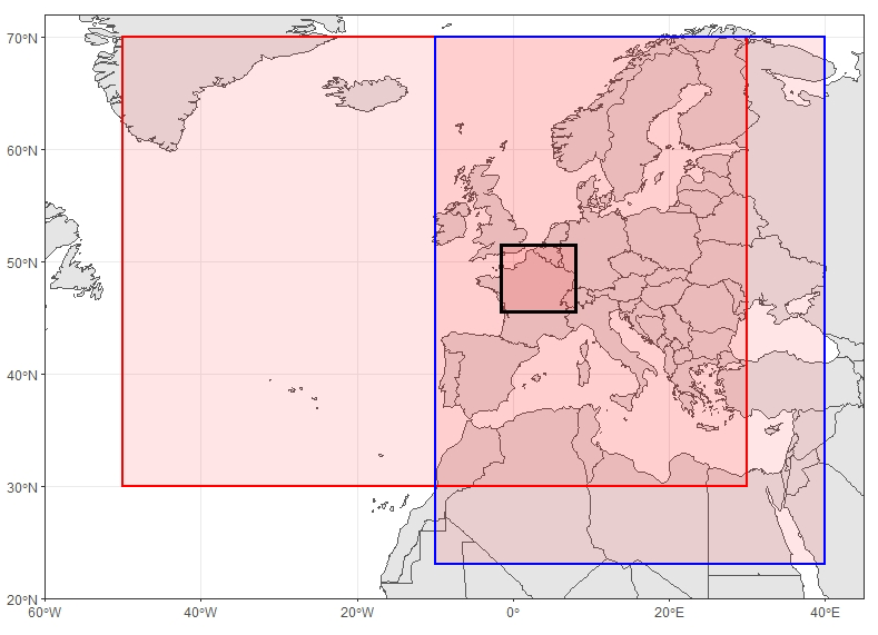
Figure 1Regions used to identify circulation analogues for December temperatures (blue) and spring precipitation (red). The black rectangle indicates the region over which temperatures and precipitation are averaged in northern France.
2.2 Stochastic weather generators and importance sampling
The idea behind importance sampling is to simulate trajectories of a physical system that optimize a criterion in a computationally efficient way. Ragone et al. (2017) used such an algorithm to simulate extreme heatwaves with an intermediate complexity climate model.
The procedure of importance sampling algorithms, say to simulate extreme heatwaves with a climate model, is to start from an ensemble of S initial conditions and compute trajectories of the climate model from those initial conditions.
An optimization “observable” is defined for the system. In this case, it can be the spatially averaged temperature or precipitation over France. The trajectories for which the observable (e.g. daily average temperature) is lowest during the first steps of simulation are deleted and replaced by small perturbations of remaining ones. In this way, each time increment of the simulations keeps the trajectories with the highest values of the observable. At the end of a simulation, one obtains S trajectories for which the observable (here average temperature over France) has been maximized. Since those trajectories are solutions of the equations of a climate model, they are necessarily physically consistent (given that the perturbations are small).
Ragone et al. (2017) argue that the probability of the simulated trajectories is controlled by a parameter that weighs the importance to the highest observable values: if one trajectory is deleted at each time step, the simulation of an ensemble of M-long trajectories has a probability of . Hence, one obtains a set of S trajectories with very low probability after M time increments at the cost of the computation of S trajectories.
For comparison purposes, if one wants to obtain S trajectories that have a low probability (p) observable, then the number of necessary “unconstrained” simulations is of the order of M∕p, so that most of those simulations are left out. Systems like weather@home (Massey et al., 2015b) that generate tens of thousands of climate simulations are just sufficient to obtain S=100 centennial heatwaves, and the number of “wasted” simulations is very high. Therefore, importance sampling algorithms are very efficient ways to circumvent this difficulty. The major caveat of this approach is that one needs to know the equations that drive the system and be able to simulate them. We use an alternative method that does not require such knowledge of the system.
We use two SWG-based circulation analogues (Yiou and Jézéquel, 2020) to simulate events of either warm temperature in December or high precipitation in spring. These SWGs resample daily weather observations in a plausible manner to simulate new weather events (Yiou, 2014).
Circulation analogues are computed on SLP (or detrended Z500) from NCEP between 1950 and 2018. For each day in 1950–2018, K=20 best analogues are determined by minimizing a spatial Euclidean distance between SLP (or Z500) maps.
As explained by Yiou and Jézéquel (2020), the SWG randomly samples analogues by weighting the analogue days with a criterion that favours high temperatures or high precipitation. Hence, the importance sampling is summarized by the procedure of giving more weight to analogues that yield temperature (or precipitation) properties. There are two types of importance sampling for the analogues, which are illustrated in Fig. 2.
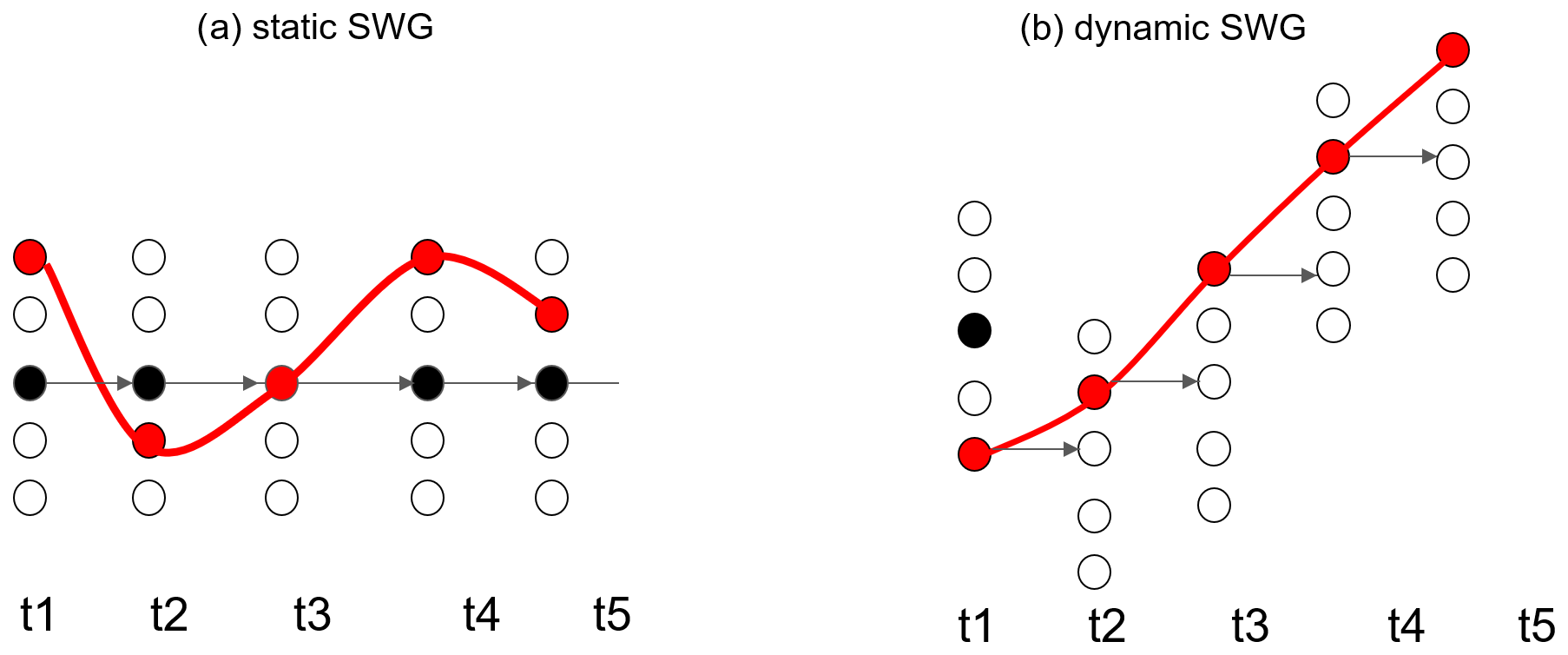
Figure 2Illustration of the analogue-based importance sampling. (a) The static SWG replaces each day in the observed trajectory (black dots) with one of its analogues (red dots). (b) The dynamic SWG replaces the first day in the observations (black dot) with one of its analogues, reads the following day of this analogue, and repeats the procedure until creating a new trajectory (red dots).
The two main types of analogue SWGs are described by Yiou (2014) and Yiou and Jézéquel (2020) are as follows:
-
A “static” weather generator replaces each day with one of its K circulation analogues or itself. With this type of SWG, simulated trajectories are perturbations (by analogues) of an observed trajectory.
-
A so-called “dynamic” weather generator has a similar random selection rule, but the “next” day to be simulated follows the selected analogue, rather than the observed actual calendar day. A probability weight ωcal that is inversely proportional to the distance to the calendar day is introduced:
where Acal is a normalizing constant, αcal≥0 is a weight, and Rcal(k) is the number of days that separate the date of kth analogue from the calendar day of time t. This rule is important to prevent time from going “backward”. This type of SWG generates new trajectories by resampling already observed ones. They are not just perturbations of observed trajectories.
Those random selections of analogues are sequentially repeated until a lead time T.
An importance sampling is applied while selecting an analogue at each time step by weighing probabilities with the variable to be optimized (temperature or precipitation). The K=20 best analogues and the day of interest are sorted by daily mean temperature or precipitation. The probability weights are determined by Yiou and Jézéquel (2020). If R(k) is the rank (in terms of temperature or precipitation) of day k in decreasing order and ωk the probability of day k to be selected, we set
where A is a normalizing constant so that the sum of weights over k is 1. The α parameter controls the strength of this importance sampling for temperature or precipitation.
The useful property of this formulation of weights is that the values of ωk do not depend on time t because the rank values R(k) are integers between 1 and K+1. The weight values do not depend on the unit of the variable either, and thus this procedure is the same for temperature or precipitation. If α=0, this is equivalent to a stochastic weather generator described by Yiou (2014).
Combining the weights of the calendar day and the intensity of the climate variable, the probability of day k to be selected becomes
The generators thus give more weight to the warmest or wettest days when computing trajectories of December temperature or spring precipitation. We thereby simulate extreme events, e.g. warm Decembers and wet springs (May to July).
2.3 Experimental set-up
The parameters of the SWG depend on the variables and the seasons to be simulated. We determine those parameters experimentally and detail them hereafter. Table 1 lists all parameters used for the simulation of December temperature and spring precipitation. These parameters were set after performing a number of sensitivity tests that are going to be discussed in Sect. 3. Table 2 lists all values tested for α and αcal. Most figures related to these tests can be found in the Appendix.
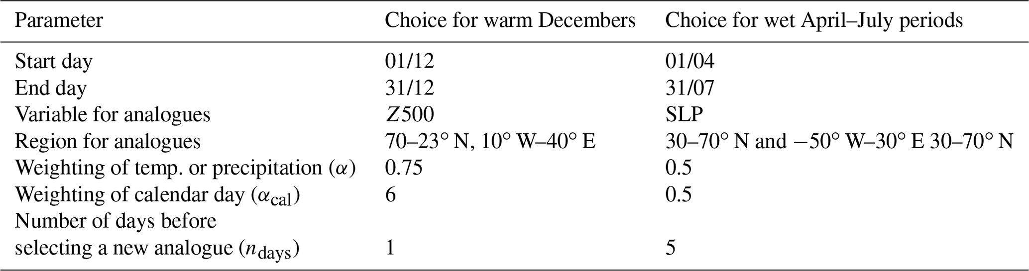
Table 1Parameters used for the static and dynamic SWG to simulate warm Decembers (second column) and wet April–July periods (last column).
The procedure we follow is as follows.
-
Start and end day of simulations. For each year from 1950 to 2018, 1000 simulations are started independently for temperature in December and precipitation in spring. The temperature simulations start on 1 December and end on 31 December. Precipitation simulations start on 1 April and end on 31 July. This results in 68 000 independent simulations of December temperatures and spring precipitation.
-
Identification of circulation analogues. Weather analogues are identified by evaluating the similarity of weather patterns of an atmospheric variable in a chosen region. For December temperature, analogues are based on detrended geopotential height at 500 hPa (Z500) over a region covering most of Europe (70–23∘ N, 10∘ W–40∘ E) (see Fig. 1). Jézéquel et al. (2018) showed that Z500 is better suited to simulate temperature anomalies than SLP and that rather small domains lead to better reconstitutions. This result is supported by sensitivity tests we performed on the choice of variable for the computation of the circulation analogues used to simulate December temperature. For spring precipitation, we use analogues of SLP over a zone covering 30–70∘ N and 50∘ W–30∘ E, as shown in Fig. 1. This region includes large parts of the North Atlantic where rain-bringing storms usually come from.
-
Number of days before selecting a new analogue. For the simulation of long-lasting precipitation events the consistency of day-to-day variability is important to ensure a plausible water vapour transport. We therefore adapt the stochastic weather generator (both static and dynamic). Instead of choosing a new analogue every day, we stay on an observed trajectory for a number of days (ndays) before choosing a new analogue (see Fig. 3). For the analogue selection we weight the analogues based on the accumulated precipitation of the analogue and the following ndays days, giving more weight to analogues that bring more precipitation in the following ndays days.
-
Selection of circulation analogues by the generators. The α-parameter controls the strength of the importance sampling on either temperature or precipitation, while αcal controls the influence of the calendar date when selecting an analogue. For temperature simulations, we use α=0.75 and αcal=6. Note that we thus strongly condition the calendar day to restrict the SWGs to winter and late autumn days. For precipitation, we set both α and αcal to 0.5.
Table 2Performed sensitivity tests for the parameters used to simulate warm Decembers (first three rows) and wet April–July periods (last three rows). The second column lists the parameters of which the sensitivity is assessed. The third column indicates at which levels all other parameters are fixed for the test. The fourth column lists all tested values and the last column indicates the figure where the results of the test are shown.

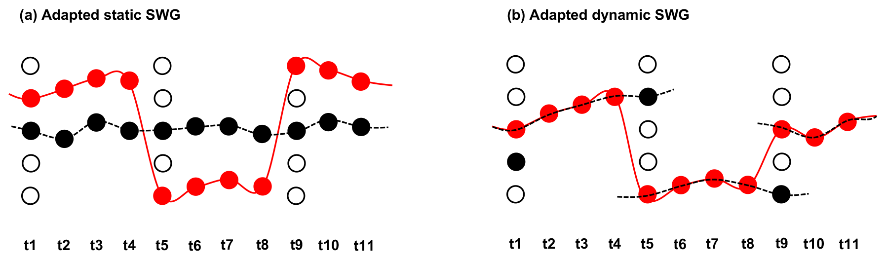
Figure 3Adapted dynamic weather generators. (a) The adapted static SWG selects a new analogue every nth day (4 d in this illustration) and follows the observed trajectory (dotted black line) of that day for 3 d. The resulting simulation combines observed 4 d chunks into an artificial trajectory (red line). (b) The adapted dynamic SWG replaces the first day of the observations with one of its analogues and follows the observed trajectory of that analogue for 3 d. Following this, a new analogue of the following day in the observed trajectory is chosen.
A lack of cold days in December 2015 and an exceptionally wet spring caused the 2016 crop loss in northern France. Although the interplay between these two meteorological events is crucial for the resulting crop loss, the two events (warm December and wet spring) seem to have happened independently from each other: the correlation between temperature in December and precipitation 4 months later is not significantly different from zero and we cannot reject the hypothesis that both variables are not correlated (p value of the Pearson correlation > 0.6). In addition, from an energy point of view, the characteristic timescale of the atmosphere does not exceed 35 d (Peixoto and Oort, 1992, Sect. 14.6.2). This implies that it is unlikely to find links between climate variables in December and the following May. We therefore consider that it is reasonable to simulate warm Decembers and wet springs independently.
3.1 December temperature simulations
The winter preceding the 2016 crop loss was abnormally warm, with only a few cold days. Here, cold days are defined as days with daily maximal temperatures between 0 and 10 ∘C. This December was the hottest in the observational record and also the December with the fewest cold days.
Figure 4a shows the observed averages of daily maximal temperatures and the results from static and dynamic SWG simulations. The observed December temperatures fluctuate around 6 ∘C, with a small warming trend of 0.2 ∘C per decade over the whole time series (p value =0.03). Simulations from the static SWG are consistently around 3.5 ∘C warmer and follow the year-to-year variability of the observations. With an average of 12 ∘C, the dynamic SWG simulations are significantly warmer than the static SWG simulations, and inter-annual variability is strongly reduced. This is to be expected as the dynamic SWG evolves freely from the starting day and is therefore less bound to each year's circulation.
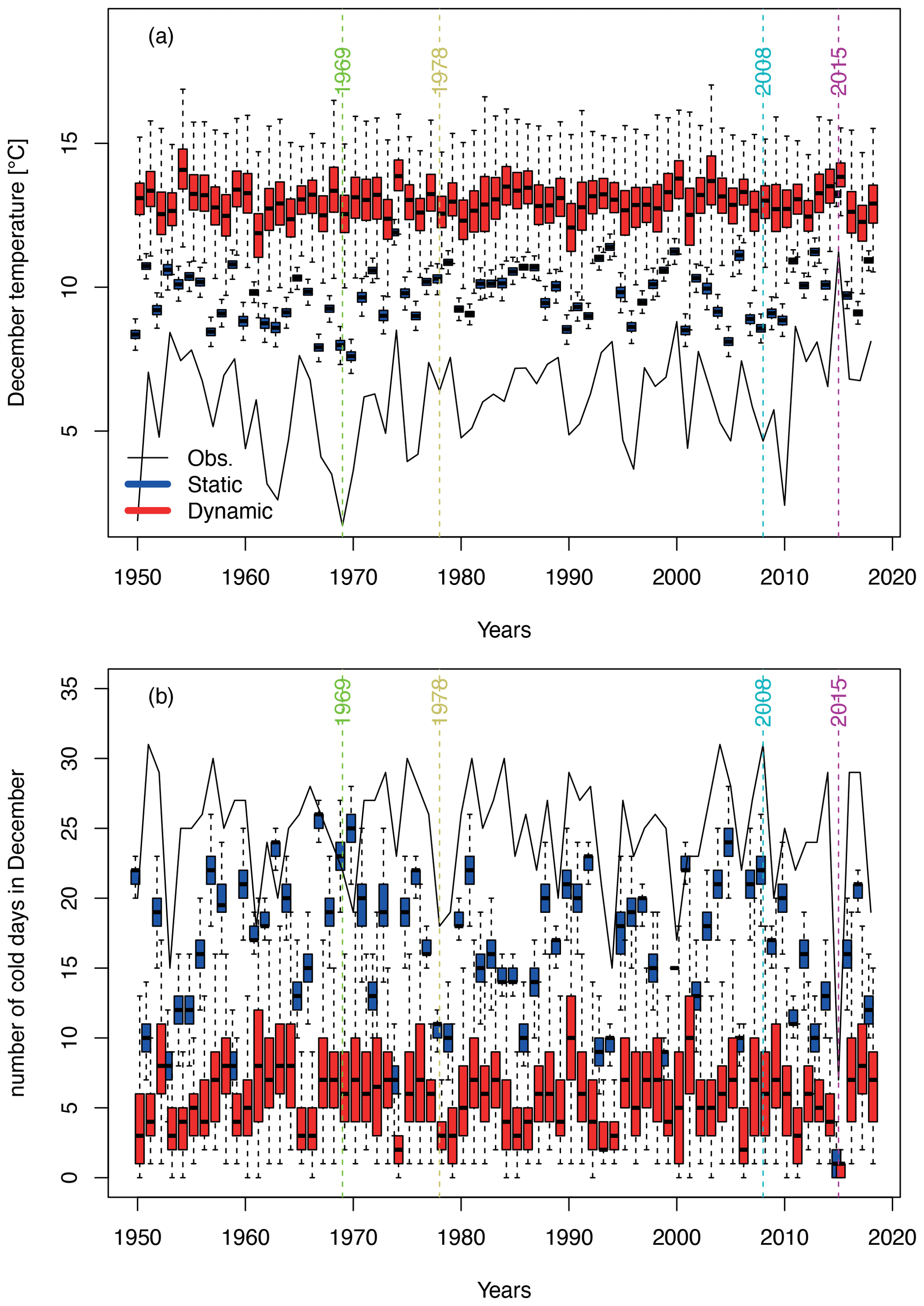
Figure 4(a) Daily maximal temperature in December from 1950 to 2018. The black line shows E-OBS observations. The boxplots represent the ensemble variability of the simulations of the static (blue) and the dynamic (red) SWG for each year. The boxes of the boxplots indicate the median (q50) and lower (q25) and upper (q75) quartiles. The upper whiskers indicate )]. The lower whisker has a symmetrical formulation. The points are the simulated values that are above or below the defined whiskers. Panel (b) is the same as (a) but for the number of cold days. The coloured vertical lines indicate the coldest December (green), a median December (yellow), a December with 31 cold days (cyan) and the warmest December (purple).
In years with higher December temperatures, the number of cold days with maximal temperatures between 0 and 10 ∘C is reduced (see Fig. 4b). Over the period 1950–2018 no trend in the number of cold days is observed and the number of cold days fluctuates around 25 d. As the SWG simulates warmer Decembers the number of cold days is on average 8 d lower in the static SWG and 16 d lower in the dynamic SWG. Nearly half of the simulations of the dynamic SWG thus have fewer cold days than what was observed in December 2015.
December 2015 was unprecedented in terms of missing cold days, and we simulate a number of warm Decembers with even fewer cold days. To estimate the probability of such an extreme December, we fit a beta-binomial distribution (Jézéquel et al., 2018) to the observations and find that 2015 was a 1-in-4000-year event and that 25 % of our dynamic SWG simulations are 1-in-1000-year events or even rarer (see Fig. A3).
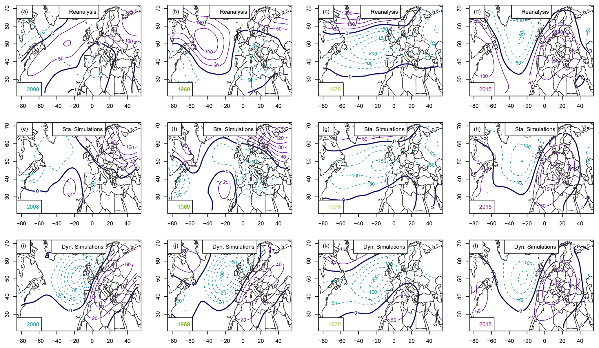
Figure 5Geopotential height anomaly at 500 hPa (Z500) composites for a year with 31 cold days (2008), the coldest December (1969), the median (1978), and the warmest December (2015): (a–c) mean Z500 from NCEP reanalyses, (d–f) static SWG simulations, (g–i) dynamic SWG simulations. Isolines are shown with 100 m increments. Positive Z500 anomalies are shown with continuous purple isolines, negative anomalies are shown with dashed cyan lines, and the 500 hPa isoline is shown with a continuous thick black line.
As shown in Fig. 5, December 2015 was characterized by a persistent anticyclonic circulation with its centre over the Alps. The circulation in the coldest December (1969) was the opposite of 2015, with negative Z500 anomalies over Europe and positive anomalies over the Atlantic. In 2008, the December with most cold days in the observations, the data resemble 1969 but have less pronounced anomalies.
For all example years, the circulation in the static SWG simulations exhibits the same features as the observed circulation. The dynamic SWG always simulates high-pressure anomalies over France irrespective of the starting conditions. These anomalies are, however, more pronounced in 2015 where the starting circulation favours the anticyclonic pattern over France.
The simulations of warm Decembers are most sensitive to the weighting of the calendar date. If this parameter is chosen too loosely, simulations would include days from other seasons, which are generally warmer. As shown in Fig. A2, for αcal≥6 over 70 % of all days in the simulations are sampled from the November–February period. Increasing the weighting of the calendar day further does not show a significant effect.
The simulations are also sensitive to the weighting of daily maximal temperatures α (Fig. A3). For α≥0.75 we simulate a large number of Decembers that are more extreme than 2015.
Finally, the choice of geopotential height or mean sea level pressure to classify circulation analogues does not influence the simulations (see Fig. A1).
3.2 Spring precipitation
An extremely wet period from April to July 2016 followed the warm December in 2015, with an average precipitation of 2.7 mm per day and 332 mm for the whole period. This is more than the long-term 75th percentile, but it is topped by some years including 1983, 1987, and 2012.
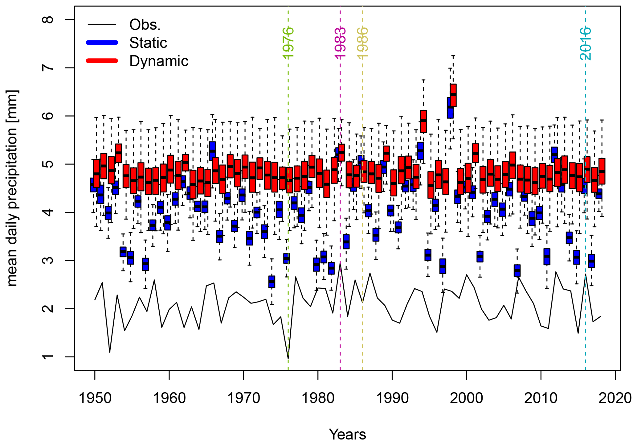
Figure 6Daily precipitation averages for April–July from 1950 to 2018. The black line shows E-OBS observations. The boxplots represent the ensemble variability of the simulations of the static (blue) and the dynamic (red) SWG for each year. The boxes of boxplots indicate the median (q50), lower (q25), and upper (q75) quartiles. The upper whiskers indicate )]. The lower whisker has a symmetrical formulation. The points are the simulated values that are above or below the defined whiskers. The coloured vertical lines indicate the driest April–July period (1976), the wettest period (1983), a median period (1986), and 2016.
Figure 6 shows the daily mean precipitation for April–July periods over 1950–2018. Accumulated April–July precipitation fluctuates around 256 mm with a strong year-to-year variability. Over the observed period no trend is detected.
Simulations from the static weather generator (blue boxplots in Fig. 6) also show a strong inter-annual variability but have significantly larger amounts of precipitation. The average seasonal precipitation for all simulations and all years is around 487 mm–190 % of the observed average. Single simulations even reach daily mean precipitation of 6 mm for April–July, which is 3 times as high as the observed precipitation in 1983.
April–July periods simulated by the dynamic SWG are even wetter than the simulations of the static SWG, with an average seasonal precipitation of 590 mm. As expected, the inter-annual variations are smaller in the dynamic SWG simulations than in the static SWG simulations because the dynamic SWG evolves freely, with the starting conditions their only link to the observed circulation.
We estimate the return periods of our simulated events by fitting a normal distribution to the observed April–July precipitation events. As we average over a quite large region and over 4 months, a normal distribution represents the observations well (even though the analysed variable is precipitation). We find that the 2016 April–July period was a 1-in-17-year event, while the majority of our SWGs simulations are 1-in-10 000-year events.
In April–July 2016, the atmospheric circulation was characterized by a moderate low-pressure anomaly north of France and north of the Azores (Fig. 7a). The North Atlantic Oscillation (NAO) index switched from slightly positive to negative in May and remained negative until the end of June (NOAA, 2020).
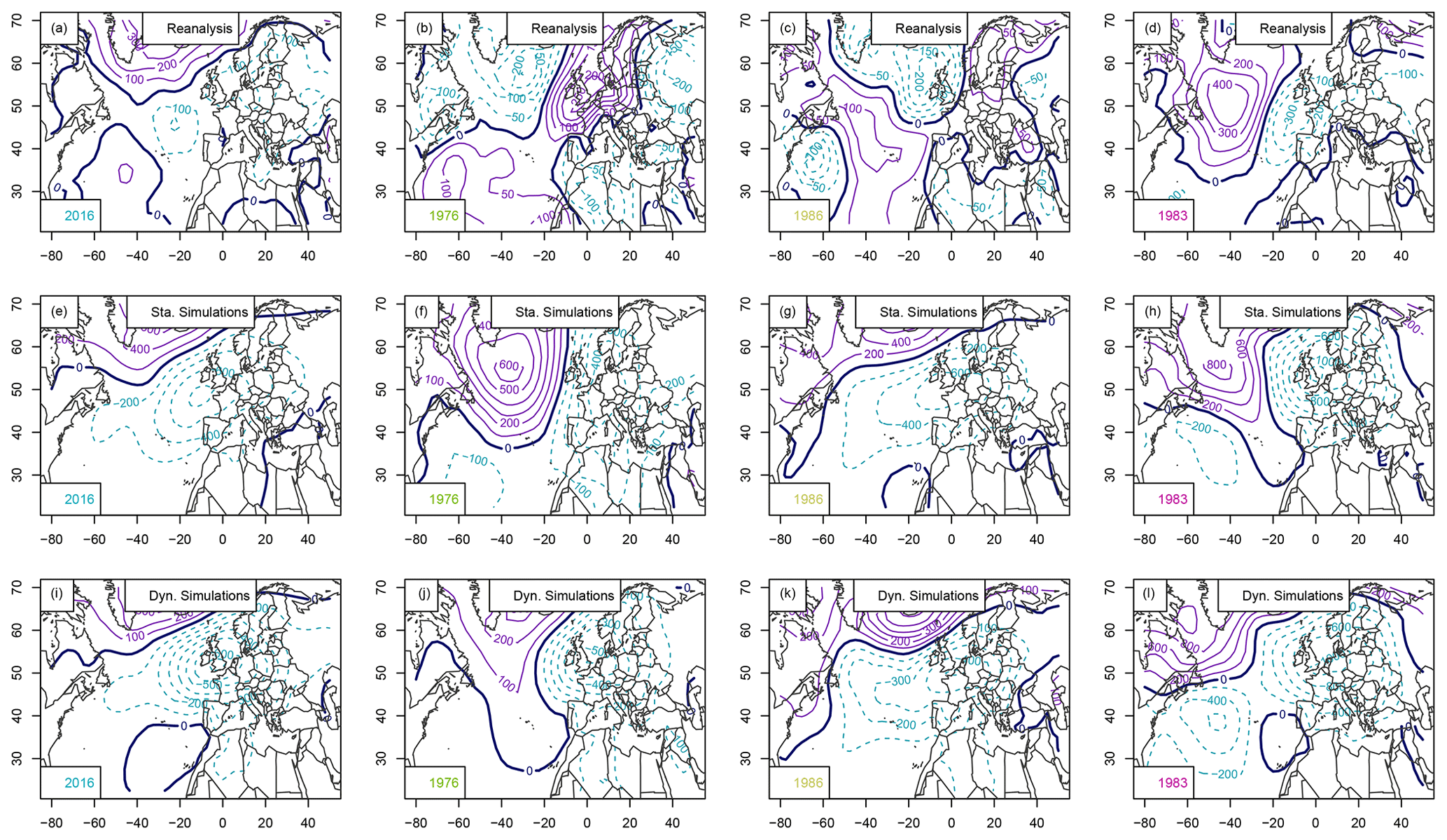
Figure 7SLP anomaly composites (Pa) for April–July 2016, the driest period, the median (1986), and the wettest period (1983): (a–d) mean SLP from NCEP reanalyses, (e–h) static SWG simulations, (i–l) dynamic SWG simulations. Isolines are shown with 100 Pa increments. Positive SLP anomalies are shown with continuous purple isolines, negative anomalies are shown with dashed cyan lines, and the mean SLP isoline is shown with a continuous thick black line.
We next analyse the large-scale atmospheric circulation patterns that characterize our SWG simulations by comparing them to a few examples of observed events. Figure 7a–d shows the mean sea level composites of 2016, the driest (1976), the median (1986), and the wettest (1983) April–July periods. The main feature in the median event (Fig. 7c) is a low pressure anomaly north-westward of the British Isles. The wettest event (Fig. 7d) is characterized by a strong dipole over the North Atlantic with low pressure in the east and high pressure in the west. In the driest event (Fig. 7b) this dipole is reversed and slightly shifted to the east.
For all four events, the static SWG tends to create events with stronger low pressure anomalies over northern France (Fig. 7e–h). Similarly, the simulations from the dynamic SWG all show a strong low-pressure anomaly over northern France (Fig. 7i–l). For the dynamic SWG simulations, even in 1976, which was the driest April–July period, a low-pressure anomaly is simulated for northern France where a high-pressure system had been observed. In the static SWG, the high-pressure anomaly is relocated to the west, also leading to a low-pressure anomaly over northern France.
Besides a general tendency towards low-pressure anomalies over northern France, the 2016 April–July period was characterized by an increased daily pressure variability west of France (compare Figs. B1a and c). This indicates an enhanced storm track activity downstream of our region of interest and could explain the increased precipitation observed in 2016. In contrast to the persistent anticyclonic anomaly that led to a continuously warm December in 2015, the wet April–July period was favoured by a number of storms passing over northern France.
Our simulations of April–July periods combine 5 d chunks of observed weather into one coherent time series. By using 5 d chunks instead of combining single-day observations, we constrain our simulations to observed day-to-day variations that appear to be crucially important for precipitation events. This ensures that in our simulations storms predominantly travel eastwards and that the moisture transport in the simulations is reasonable – at least during the 5 d in question (see the animated .gif files in the Supplement).
Sensitivity tests indeed show that simulations where a new analogue is chosen every day result in significantly higher precipitation, with 7 mm per day for the dynamic SWG simulations (see Fig. A4). The amount of precipitation steadily decreases with the length of the observed chunks that are assembled by the SWGs (ndays). This is to be expected, as with longer assembled chunks and fewer analogue choices the simulated weather events resemble the observations more and more. There is an especially strong decrease in simulated precipitation from 1 to 3 d, which suggests that when analogues are chosen more frequently than every third day potentially unreasonable weather events are created. Note that taking 5 d windows is a heuristic choice and that window sizes between 4 and 7 d give similar results.
The simulations are by definition sensitive to the weighting of the amount of precipitation α. As shown in Fig. A5, with a relatively small weight of 0.1 most dynamic simulations already bring more precipitation than what was observed in 2016. This could be due to the length of the simulations: it is rather unlikely that extreme weather endures over 4 months. However, with a weak weighting of wet weather simulations can already result in a long-lasting consistent wet periods. This increase in precipitation saturates after α≈0.5, and increasing α further has no effect on the final results.
As for the other free parameters of the SWG, this sensitivity test does not directly justify the choice of the parameter α. It instead gives guidance on the values that would be appropriate choices for our application. In the end the parameter is heuristically chosen considering the trade-off between creating high-precipitation events and keeping as much randomness as possible in our simulations.
As shown in Fig. A6, the weighting of the calendar day has limited influence on the amount of precipitation in northern France simulated by our SWGs.
For precipitation in northern France the weighting of the calendar day is less relevant as there is no pronounced seasonal cycle in precipitation (see Fig. A6).
Finally, one feature in the simulations of April–July deserves some more attention: for both static and dynamic SWG simulations precipitation is exceptionally high in 1994 and 1998. Although observed precipitation in these years was relatively high, this cannot explain the amount of precipitation in the simulations. One explanation for these outlier years could be a loop in the simulations leading to an excessive repetition of the same (wet) sequence of days. As shown in Fig. A7, in 1998 one date is indeed repeated 10 times in both the static and dynamic weather generator. In most other years, repetitions of single dates are rare. As our results do not rely on simulations of single years, this feature does not affect the overall findings of the study.
These simulations show that there are many possible April–July periods that would be significantly wetter than what was observed in 2016 and also wetter than the observed record precipitation (1983).
In 2016 northern France suffered an unprecedented crop loss that can be related to an abnormally warm December in 2015 and a following wet April–July period in 2016 (Ben-Ari et al., 2016). Here we investigated how extreme these meteorological precursors of the crop loss could be in the current climate. Using stochastic weather generators (SWG) we simulate warm Decembers and wet April–July periods independently.
The warm December in 2015 resulted in very few cold days with temperatures between 0 and 10 ∘C. Our simulations show that substantially warmer Decembers would be possible. However, in terms of cold days, which is a more relevant indicator for wheat phenology in that season (Ben-Ari et al., 2018), December 2015 was already extreme, and only a few simulations show lower numbers of cold days.
For April–July precipitation, we find that much wetter periods than what was observed in 2016 would be plausible. The simulated events bring more than twice as much precipitation than in 2016.
If crop yields responds to the number of cold days in winter and to the precipitation rate in spring, as shown in Ben-Ari et al. (2018), then we have shown here that in the current climate an even worse crop loss event would be possible. The April–July period in particular could be significantly wetter than what was observed in 2016.
We used stochastic weather generators to simulate extreme but plausible weather events. While the method is established for summer heat waves (Yiou and Jézéquel, 2020), the weather events we studied here brought new challenges: although the circulation pattern of the warm December 2015 was similar to a summer heat wave with an anticyclonic pattern over France, special care was required to assure that our simulated events are actually realizations of winter weather. Here we assured for this by strongly weighting the calendar date when selecting analogues.
The wet April–July 2016 period was characterized by a series of passing storms that brought considerable amounts of precipitation. The main feature of this wet spring season was therefore not persistence and simulating plausible day-to-day variations with SWGs was a major challenge. SWGs that select a new analogue every day tend to simulate persistent rainfall events over spring, with little day-to-day variation.
As a first attempt to simulate plausible long lasting wet periods, we propose to reassemble 5 d windows of observed weather instead of single days. This ensures that low- and high-pressure systems predominantly travel eastward at a speed that is tightly linked to observations. An alternative approach could be to switch trajectories on dry days instead of switching after a fixed number of days. This would additionally avoid changing trajectories during precipitation events.
Evaluating the plausibility of our simulations remains a challenge: although sensitivity tests and an analysis of the simulated circulation patterns reveal the robust and clearly interpretable behaviour of SWGs, further tests would be required to assess whether all simulated events could really happen in our climate. It could, for instance, be interesting to analyse the simulated wet April–July periods with respect to more climate variables (e.g. relative humidity) to evaluate whether the water transport is physically plausible throughout the simulated period.
To further evaluate the plausibility of our simulations one could also compare them to extreme events simulated by large ensemble climate modelling experiments. In a study using a near-term climate prediction model, Thompson et al. (2017) found that for England there is a considerable chance of unprecedented winter rainfall. Replicating a similar study for northern France spring precipitation would not only provide an alternative estimate of extreme spring precipitation but would also allow us to further evaluate the circulation features of our weather simulations.
Finally, our simulated extremes could be used as input for the regression-based yield model of Ben-Ari et al. (2018). These results should, however, be interpreted cautiously as our simulated weather extremes lie outside of the observed range and therefore also the range within which the yield model was trained. They could also be used in process-based crop models as a worst-case meteorological scenario.
This paper is a proof of concept for the importance sampling for a simulation of a compound event (warm autumn-winter and wet spring) that would have an impact on crop yield. It relies on a data-resampling approach to maximize temperature and precipitation over extended periods of time.
The simulations are based on the a priori knowledge (from expertise on crop failures in northern France) that warm autumns and winters followed by wet springs have detrimental effects on crops.
The first application of SWGs to warm winter periods and wet springs is an important advance in this research field. It also shows that with only a few adaptations SWGs can be applied to new weather phenomena, highlighting the merits of the method. Moreover, the SWG parameters can be adapted to other types of crops (with other phenological parameters and key dates).
This approach is rather flexible and could be adapted to simulate compound extremes using climate model outputs based on different scenarios of climate change. This could lead to the first evaluation of the impact of climate change on worst-case scenarios of crop yields. This type of analysis has some limitations related to the uncertainty of models and scenarios, and it fails to take into account non-climatic drivers of crop yields such as pests, supply chains, or economical concerns. However, we believe it could be useful to estimate what could be plausible in terms of purely meteorological events in a changing climate.
A1 December temperature
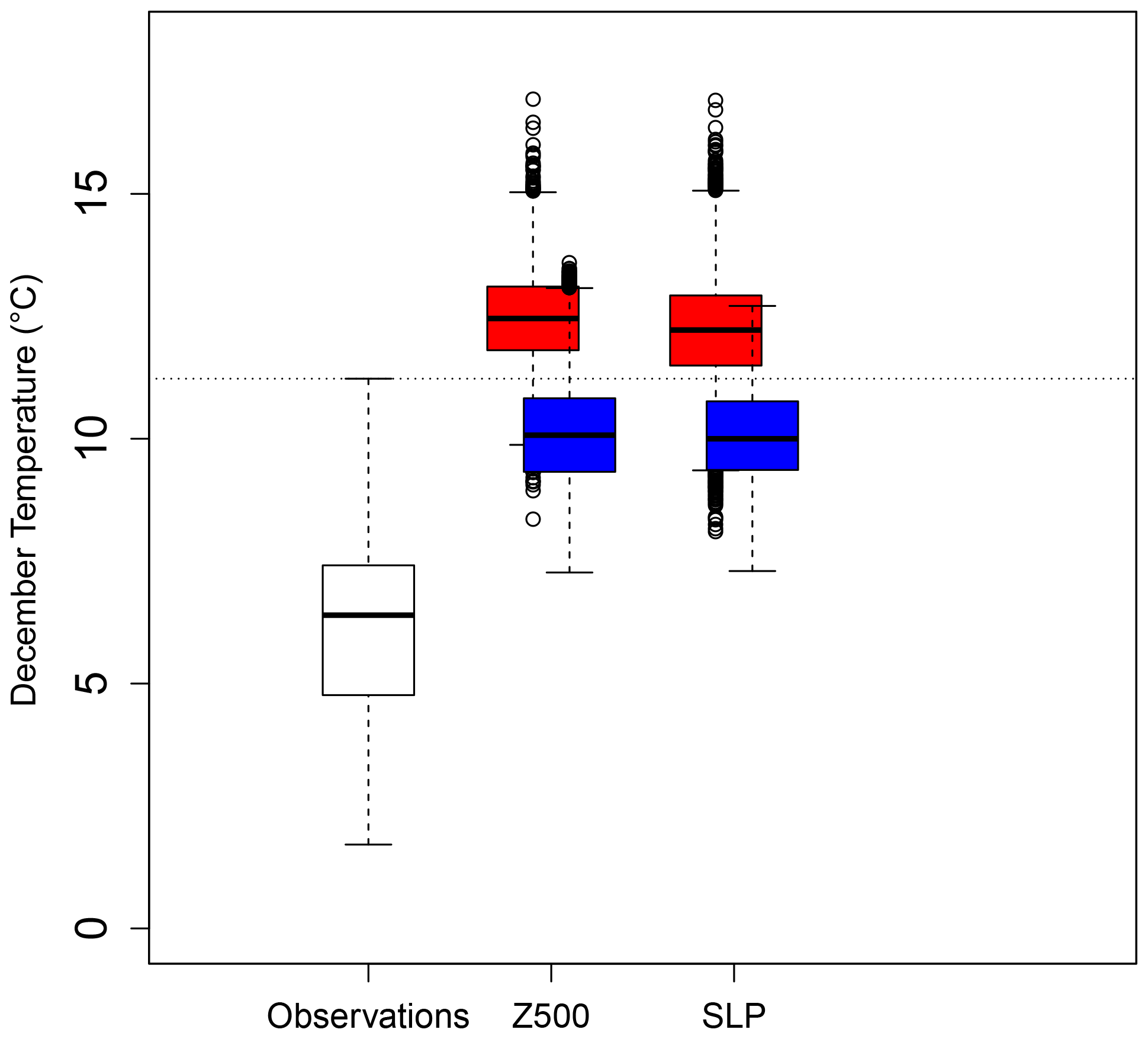
Figure A1Distribution of the daily maximum temperature in December averaged in observations (white) and in simulations computed by the static (blue) and dynamic (red) generators using circulation analogues computed using the SLP or Z500. The horizontal dotted line corresponds to the daily maximum temperature observed in December 2015. The boxes of boxplots indicate the median (q50), lower (q25), and upper (q75) quantiles. The upper whiskers indicate min[max(T),1.5×(q75−q25)]. The lower whisker has a symmetrical formulation. The points are the simulated values that are above or below the defined whiskers.
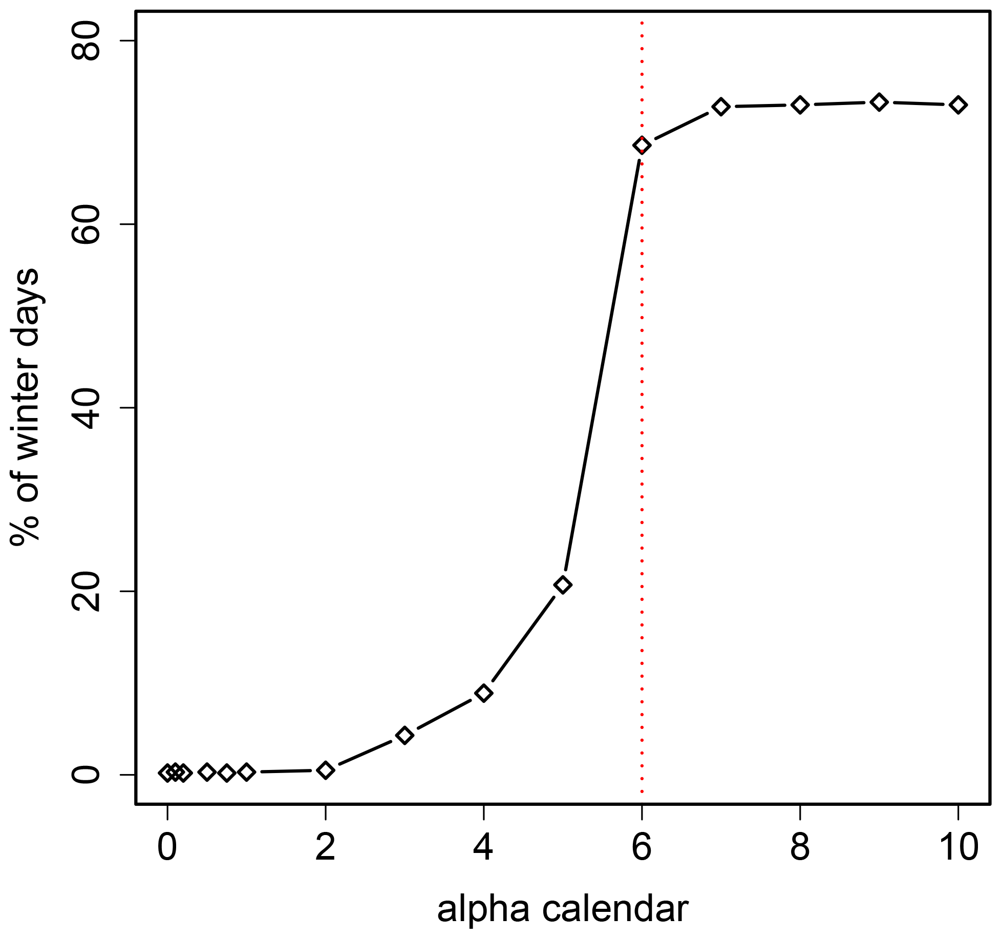
Figure A2Percentage of days sampled between November and February by the dynamic generator when running 100 simulations of December temperatures as a function of the parameter αcal. The dotted red line is for αcal=6 (which is the value used in the analysis).
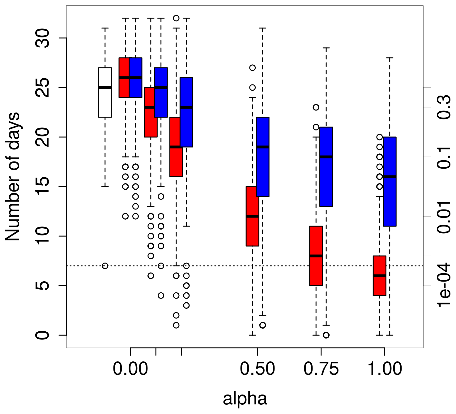
Figure A3Distribution of the number of December days with maximal temperatures between 0 and 10 ∘C in observations (white) and in simulations computed by the static (blue) and dynamic (red) generators as a function of α. The axis on the right indicates the probability of occurrence, assuming a beta-binomial distribution of the number of winter days with parameters estimated from white boxplot. The horizontal dotted line corresponds to the observed number of days in December 2015. The boxes of boxplots indicate the median (q50), lower (q25), and upper (q75) quartiles. The upper whiskers indicate min[max(T), )]. The lower whisker has a symmetrical formulation. The points are the simulated values that are above or below the defined whiskers.
A2 Spring precipitation
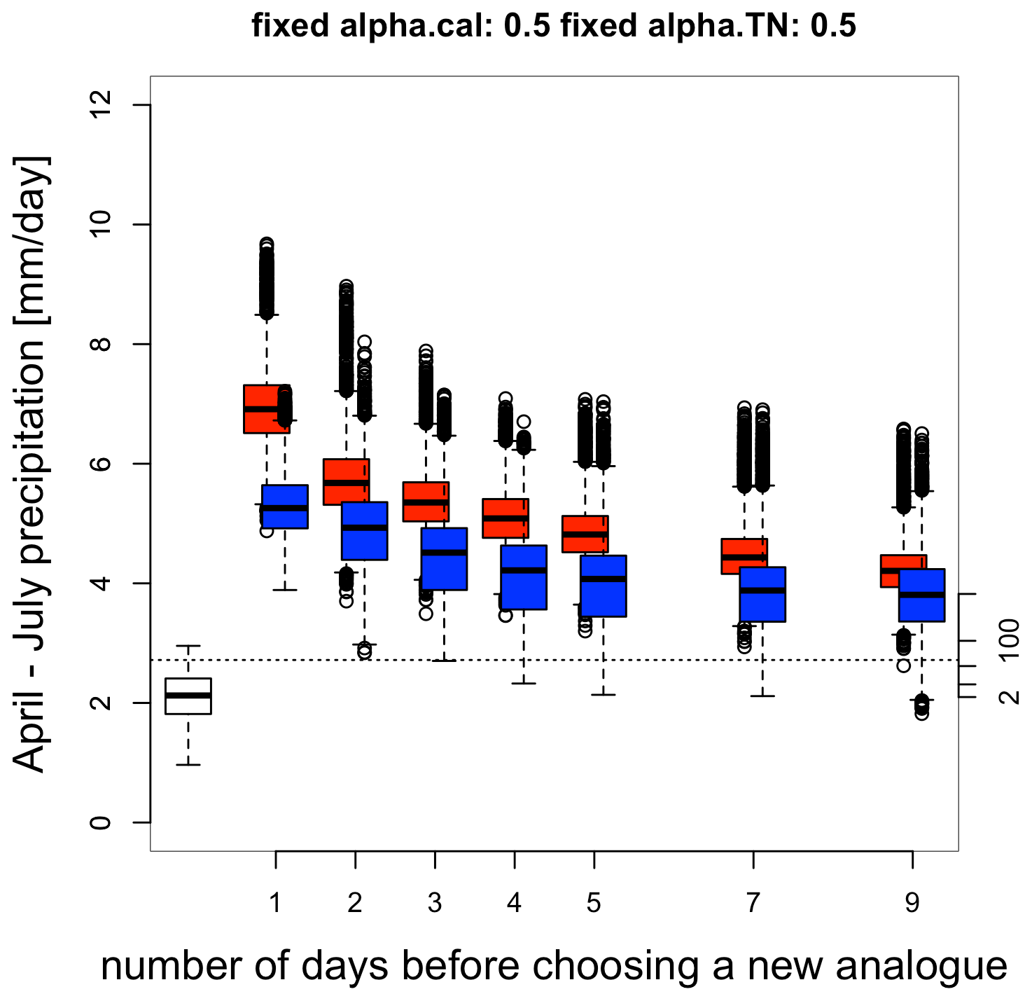
Figure A4Distribution of April–July daily precipitation in observations (white) and in simulations computed by the static (blue) and dynamic (red) generators as a function of the number of days before selecting a new analogue ndays. The axis on the right indicates the probability of occurrence, assuming a normal distribution of daily precipitation with parameters estimated from white boxplot. The horizontal dotted line corresponds to the observed daily precipitation in April–July 2016. The boxes of boxplots indicate the median (q50), lower (q25), and upper (q75) quartiles. The upper whiskers indicate min[max(T), )]. The lower whisker has a symmetrical formulation. The points are the simulated values that are above or below the defined whiskers.
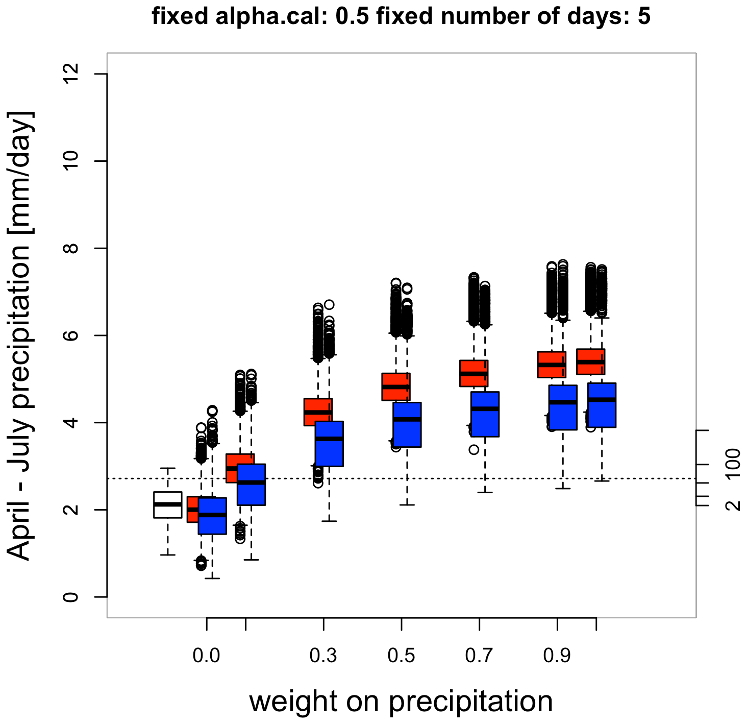
Figure A5Distribution of April–July daily precipitation in observations (white) and in simulations computed by the static (blue) and dynamic (red) generators as a function of α. The axis on the right indicates the probability of occurrence, assuming a normal distribution of daily precipitation with parameters estimated from white boxplot. The horizontal dotted line corresponds to the observed daily precipitation in April–July 2016. The boxes of boxplots indicate the median (q50), lower (q25), and upper (q75) quartiles. The upper whiskers indicate min[max(T), )]. The lower whisker has a symmetrical formulation. The points are the simulated values that are above or below the defined whiskers.
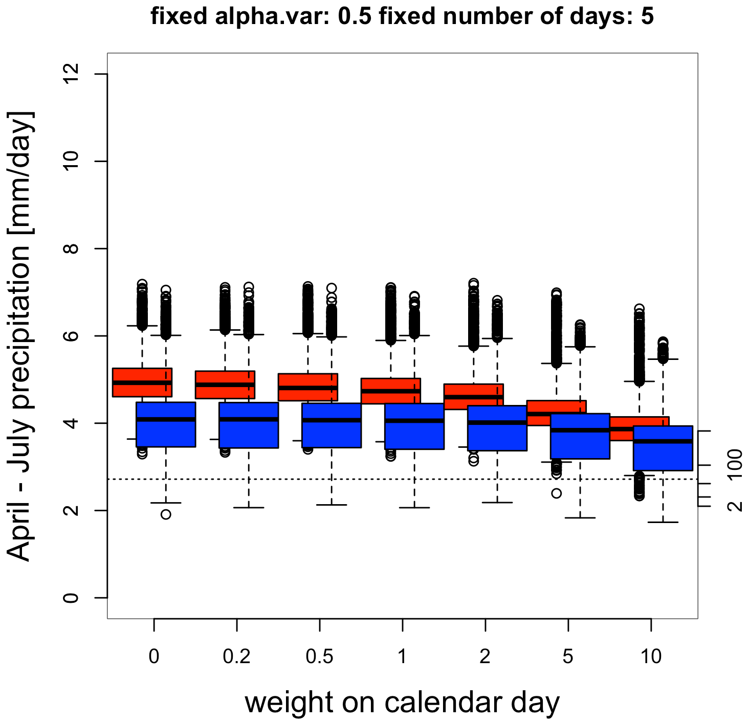
Figure A6Distribution of April–July daily precipitation in observations (white) and in simulations computed by the static (blue) and dynamic (red) generators as a function of αcal. The axis on the right indicates the probability of occurrence, assuming a normal distribution of daily precipitation with parameters estimated from the white boxplot. The horizontal dotted line corresponds to the observed daily precipitation in April–July 2016. The boxes of boxplots indicate the median (q50), lower (q25), and upper (q75) quartiles. The upper whiskers indicate min[max(T), )]. The lower whisker has a symmetrical formulation. The points are the simulated values that are above or below the defined whiskers.
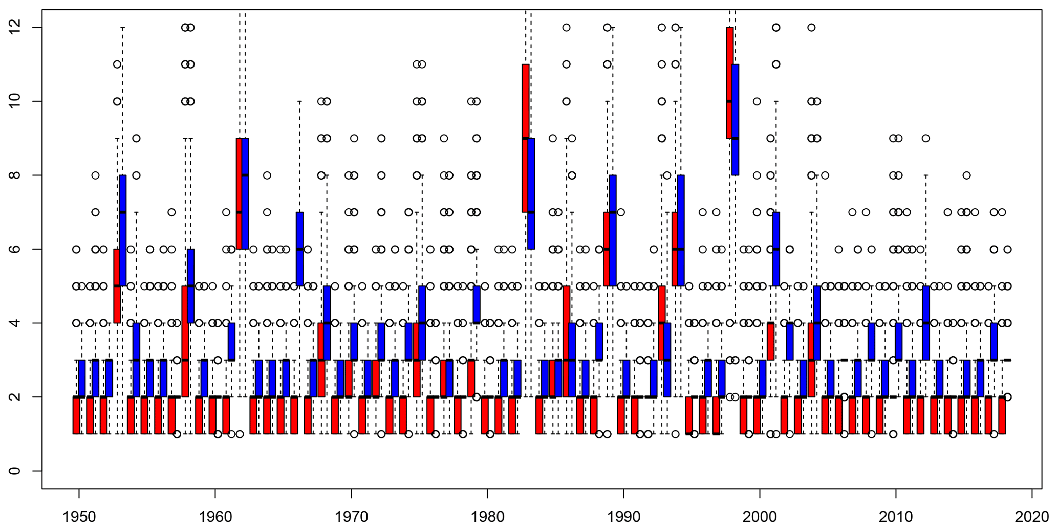
Figure A7Maximal number of times a single date is repeated for each simulated year. The boxplots indicate the range of this maximal repetition number for the 1000 simulations for simulations of the static (blue) and dynamic (red) stochastic weather generator. The boxes of boxplots indicate the median (q50), lower (q25), and upper (q75) quartiles. The upper whiskers indicate min[max(T), )]. The lower whisker has a symmetrical formulation. The points are the simulated values that are above or below the defined whiskers.
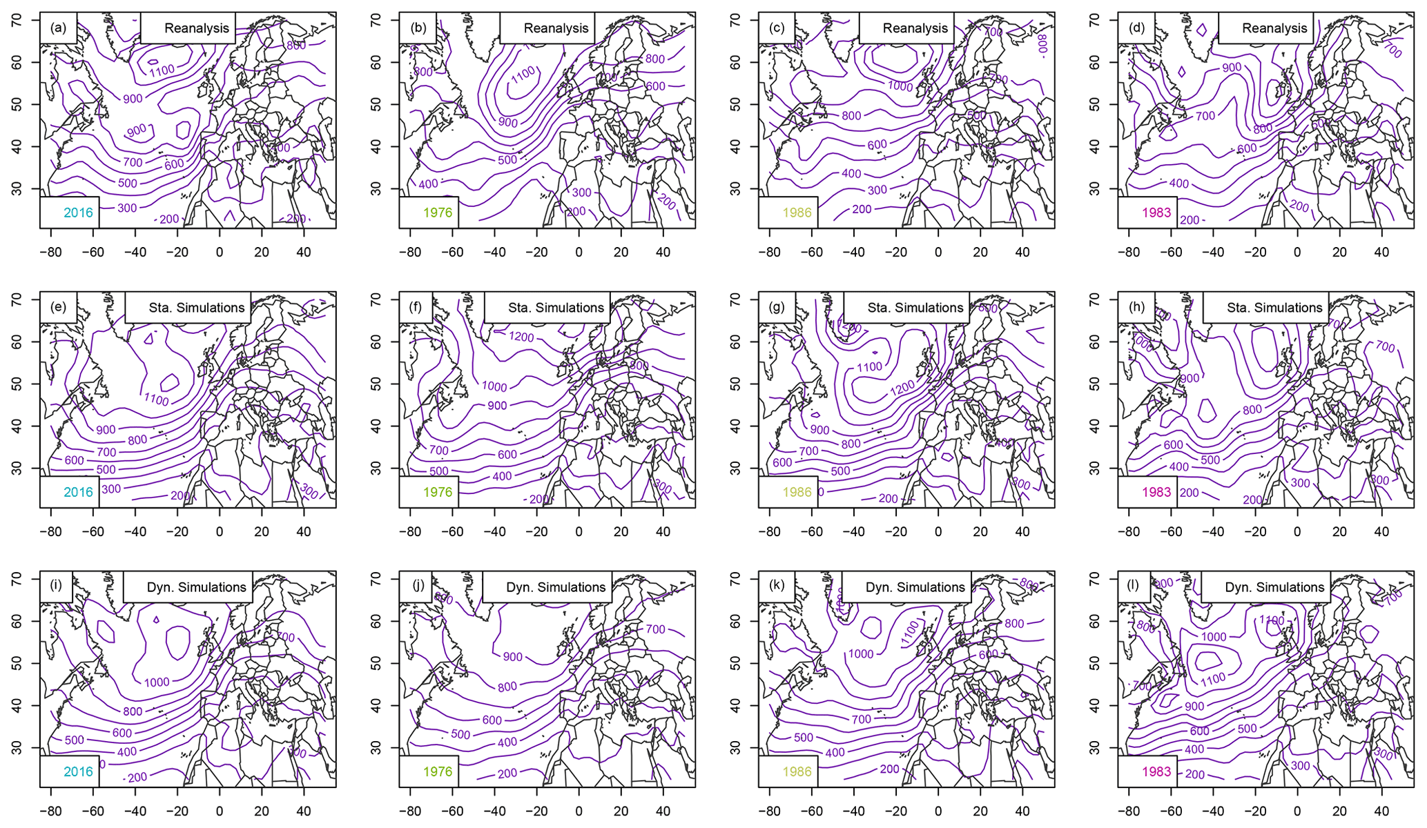
Figure B1Standard deviation of daily SLP anomalies (Pa) for April–July 2016, the driest period, the median (1986), and 2018: (a–d) SLP from NCEP reanalyses, (e–h) static SWG simulations, (i–l) dynamic SWG simulations. For the SWG simulations the average of all 1000 runs for the given year is presented.
All R scripts used for the analysis and the production of figures are openly available under https://doi.org/10.5281/zenodo.4327671 (Pfleiderer et al., 2020).
The supplement related to this article is available online at: https://doi.org/10.5194/esd-12-103-2021-supplement.
PY and AJ conceived the study. NL, JL, IM, EV, and PP did the analysis and created all figures. PP wrote the manuscript with contributions from all authors.
The authors declare that they have no conflict of interest.
This article is part of the special issue “Understanding compound weather and climate events and related impacts (BG/ESD/HESS/NHESS inter-journal SI)”. It is not associated with a conference.
We acknowledge the E-OBS dataset from the EU-FP6 project UERRA (http://www.uerra.eu, last access: 20 September 2019) and the Copernicus Climate Change Service and the data providers of the ECAD project (https://www.ecad.eu, last access: 20 September 2019). We also acknowledge the NCEP Reanalysis data provided by the NOAA/OAR/ESRL.
This research has been supported by the DAMOCLES COST (grant no. CA17109). Peter Pfleiderer was supported by the German Federal Ministry of Education and Research (grant no. 01LN1711A). Edoardo Vignotto was supported by the Swiss National Science Foundation (Doc.CE11 Mobility Grant no. 188229).
The publication of this article was funded by the
Open Access Fund of the Leibniz Association.
This paper was edited by Bart van den Hurk and reviewed by Daithi Stone and Henrique Moreno Dumont Goulart.
ARVALIS: Rendements catastrophiques du blé en 2016: la pluie, seule responsable?, available at: https://www.semencesdefrance.com/actualite-semences-de-france/rendements-catastrophiques-ble-2016-pluie-seule-responsable/ (last access: 23 October 2020), 2016 (in French). a
Ben-Ari, T., Adrian, J., Klein, T., Calanca, P., Van der Velde, M., and Makowski, D.: Identifying indicators for extreme wheat and maize yield losses, Agr. Forest Meteorol., 220, 130–140, 2016. a
Ben-Ari, T., Boé, J., Ciais, P., Lecerf, R., Van der Velde, M., and Makowski, D.: Causes and implications of the unforeseen 2016 extreme yield loss in the breadbasket of France, Nat. Commun., 9, 1627, https://doi.org/10.1038/s41467-018-04087-x, 2018. a, b, c, d, e, f, g, h, i
Cassou, C., Terray, L., and Phillips, A. S.: Tropical Atlantic influence on European heat waves, J. Climate, 18, 2805–2811, 2005. a
Cooley, D.: Extreme value analysis and the study of climate change, Climatic Change, 97, 77–83, 2009. a
de Bruijn, K. M., Lips, N., Gersonius, B., and Middelkoop, H.: The storyline approach: a new way to analyse and improve flood event management, Nat. Hazards, 81, 99–121, https://doi.org/10.1007/s11069-015-2074-2, 2016. a
FAO: Agricultural statistics database, Rome: World Agricultural, Information Center, available at: http://faostat.fao.org/site/567/DesktopDefault.aspx (last access: 22 May 2020), 2013. a
Haylock, M. R., Hofstra, N., Tank, A. M. G. K., Klok, E. J., Jones, P. D., and New, M.: A European daily high-resolution gridded data set of surface temperature and precipitation for 1950–2006, J. Geophys. Res.-Atmos., 113, D20119, https://doi.org/10.1029/2008JD010,201, 2008. a
Hazeleger, W., Van Den Hurk, B. J., Min, E., Van Oldenborgh, G. J., Petersen, A. C., Stainforth, D. A., Vasileiadou, E., and Smith, L. A.: Tales of future weather, Nat. Clim. Change, 5, 107–113, https://doi.org/10.1038/nclimate2450, 2015. a, b
Jaworski, P., Durante, F., Hardle, W. K., and Rychlik, T.: Copula theory and its applications, vol. 198, Springer, Berlin, Heidelberg, 2010. a
Jézéquel, A., Cattiaux, J., Naveau, P., Radanovics, S., Ribes, A., Vautard, R., Vrac, M., and Yiou, P.: Trends of atmospheric circulation during singular hot days in Europe, Environ. Res. Lett., 13, 054007, https://doi.org/10.1088/1748-9326/aab5da, 2018. a, b
Kistler, R., Kalnay, E., Collins, W., Saha, S., White, G., Woollen, J., Chelliah, M., Ebisuzaki, W., Kanamitsu, M., Kousky, V., van den Dool, H., Jenne, R., and Fiorino, M.: The NCEP-NCAR 50-year reanalysis: Monthly means CD-ROM and documentation, B. Am. Meteor. Soc., 82, 247–267, 2001. a
MacDonald, R. B. and Hall, F. G.: Global crop forecasting, Science, 208, 670–679, 1980. a
Massey, N., Jones, R., Otto, F., Aina, T., Wilson, S., Murphy, J., Hassell, D., Yamazaki, Y., and Allen, M.: weather@ home–development and validation of a very large ensemble modelling system for probabilistic event attribution, Q. J. Roy. Meteor. Soc., 141, 1528–1545, 2015a. a
Massey, N., Jones, R., Otto, F. E. L., Aina, T., Wilson, S., Murphy, J. M., Hassell, D., Yamazaki, Y. H., and Allen, M. R.: weather@home–development and validation of a very large ensemble modelling system for probabilistic event attribution, Q. J. Roy. Met. Soc., 141, 1528–1545, https://doi.org/10.1002/qj.2455, 2015b. a
Müller, C., Elliott, J., Kelly, D., Arneth, A., Balkovic, J., Ciais, P., Deryng, D., Folberth, C., Hoek, S., Izaurralde, R. C., Jones, C. D., Khabarov, N., Lawrence, P., Liu, W., Olin, S., Pugh, T. A. M., Reddy, A., Rosenzweig, C., Ruane, A. C., Sakurai, G., Schmid, E., Skalsky, R., Wang, X., de Wit, A., and Yang, H.: The Global Gridded Crop Model Intercomparison phase 1 simulation dataset, Scientific Data, 6, 1–22, 2019. a
NOAA: North Atlantic Oscillation, available at: https://www.cpc.ncep.noaa.gov/products/precip/CWlink/pna/nao.shtml, last access: 10 January 2020. a
OEC: The Observatory of Economic Complexity, available at: https://oec.world/en/, last access: 23 April 2020. a
Peixoto, J. P. and Oort, A. H.: Physics of Climate: New York, American Institute of Physics, New York, United States, 520 pp., 1992. a
Pfleiderer, P., Jézéquel, A., Legrand, J., Legrix, N., Markantonis, I., Vignotto, E., and Yiou, P.: analogues_of_2016_crop_failure_in_France, Zenodo, https://doi.org/10.5281/zenodo.4327671, 2020. a
Ragone, F., Wouters, J., and Bouchet, F.: Computation of extreme heat waves in climate models using a large deviation algorithm, P. Natl. Acad. Sci. USA, 115, 24–29, 2017. a, b, c
Shepherd, T. G.: Storyline approach to the construction of regional climate change information, P. Roy. Soc A-Math. Phy., 475, 20190013, https://doi.org/10.1098/rspa.2019.0013, 2019. a, b
Shepherd, T. G., Boyd, E., Calel, R. A., Chapman, S. C., Dessai, S., Dima-West, I. M., Fowler, H. J., James, R., Maraun, D., Martius, O., Senior, C. A., Sobel, A. H., Stainforth, D. A., Tett, S. F., Trenberth, K. E., van den Hurk, B. J., Watkins, N. W., Wilby, R. L., and Zenghelis, D. A.: Storylines: an alternative approach to representing uncertainty in physical aspects of climate change, Climatic Change, 151, 555–571, https://doi.org/10.1007/s10584-018-2317-9, 2018. a
Sturaro, G.: A closer look at the climatological discontinuities present in the NCEP/NCAR reanalysis temperature due to the introduction of satellite data, Clim. Dynam., 21, 309–316, https://doi.org/10.1007/s00382-003-0334-4, 2003. a
Thompson, V., Dunstone, N. J., Scaife, A. A., Smith, D. M., Slingo, J. M., Brown, S., and Belcher, S. E.: High risk of unprecedented UK rainfall in the current climate, Nat. Commun., 8, 1–6, https://doi.org/10.1038/s41467-017-00275-3, 2017. a
Yiou, P.: AnaWEGE: a weather generator based on analogues of atmospheric circulation, Geosci. Model Dev., 7, 531–543, https://doi.org/10.5194/gmd-7-531-2014, 2014. a, b, c, d
Yiou, P. and Jézéquel, A.: Simulation of extreme heat waves with empirical importance sampling, Geosci. Model Dev., 13, 763–781, https://doi.org/10.5194/gmd-13-763-2020, 2020. a, b, c, d, e, f, g, h, i
Yiou, P. and Nogaj, M.: Extreme climatic events and weather regimes over the North Atlantic: When and where?, Geophys. Res. Lett., 31, L07202, https://doi.org/10.1029/2003GL019119, 2004. a
Zscheischler, J., Martius, O., Westra, S., Bevacqua, E., Raymond, C., Horton, R. M., van den Hurk, B., AghaKouchak, A., Jézéquel, A., Mahecha, M. D., Maraun, D., Ramos, A. M., Ridder, N. N., Thiery, W., and Vignotto, E.: A typology of compound weather and climate events, Nat. Rev. Earth Environ., 1, 333–347, https://doi.org/10.1038/s43017-020-0060-z, 2020. a