2.1 Driving data

RCMs need climate information at their lateral boundaries. Here, outputs of a series of equilibrium climate simulations performed in a model chain of the Community Earth System Model (CESM 1.2 version, Hurrell et al., 2013) are used. CESM is a state-of-the-art Earth system model (ESM) consisting of different model components for the description of the atmosphere, land surface, ocean, and sea ice. In a first step, a fully coupled simulation at a horizontal resolution of 1.9° × 2.5° for the atmospheric and the land components and of nominal 1° × 1° for the ocean and the sea-ice components are executed (Buzan et al., 2023). Then, time-varying sea-ice mask and sea surface temperatures are derived from the simulation and are prescribed, in a successive step, to another experiment using only the atmosphere and land components of the CESM over an integration time of 24 years, at a horizontal resolution of 1.25° × 0.9°. Through these two steps, it is possible to reach a high spatial resolution, allowing for a realistic representation of the large-scale atmospheric circulation (Merz et al., 2015) while keeping the computational costs low.

For all of the CESM LGM simulations employed in this study, values of the orbital parameters (obliquity 22.949°, eccentricity 0.018994, and precession 294.425°), greenhouse gas concentrations (CO₂ 190 ppm, CH₄ 375 ppb, N₂O 200 ppb), and land use changes for the corresponding period at 21 ka are used following the directives of the Paleoclimate Model Intercomparison Project 4 (PMIP4, Kageyama et al., 2017).

The reference simulation is performed using the ICE-6G ice-sheet reconstruction of Peltier et al. (2015), the modification of which follows the setup for the LGM PIMP4 protocol (Zhu et al., 2017). Moreover, three additional sensitivity experiments are performed (Buzan et al., 2023), where only the ice-sheet height of the main Northern Hemisphere ice sheets (Laurentide, Greenland, Fennoscandia) is varied, respectively, to 33 %, 67 %, and 125 % of their height as derived from the dataset of Peltier et al. (2015). Additional details on the CESM model set up are presented in Buzan et al. (2023).

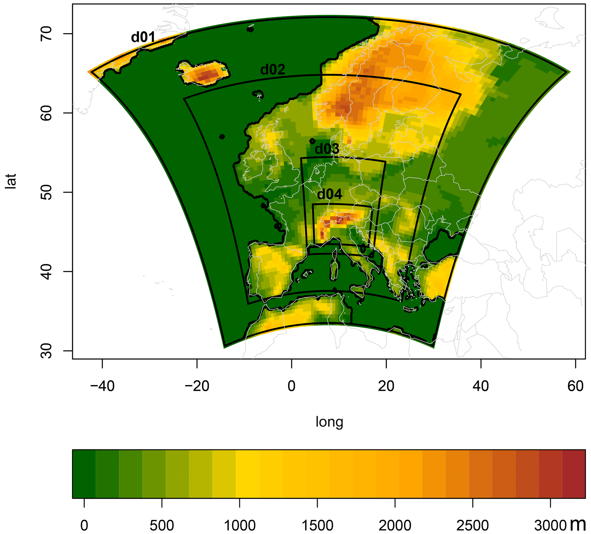
Figure 1Maps of the topography and the different nested simulation domains.

2.2 WRF general model setup

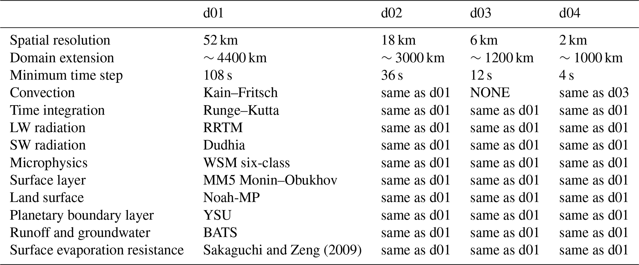
The setup of the performed WRF simulations is partly based on the same model setup of earlier studies using the same model version 3.8.1 (Velasquez et al., 2020, 2021, 2022). This setup considers four two-way nested domains, with horizontal resolutions of 54, 18, 6, and 2 km, respectively (Fig. 1). The domains cover the entire European region, with a focus on the Alps. For the time integration, an adaptive time step is used with a minimum time step of 108, 36, 12, and 4 s, respectively, for the domains going from coarser to higher resolutions. The simulations are conducted considering a total of 40 vertical eta levels in the atmosphere, and four layers in the soil, with varying vertical resolution. The Kain–Fritsch cumulus convection scheme (Kain and Fritsch, 1990, 1993; Kain, 2004) is used for the coarser domains d01 and d02 of Fig. 1. In the inner domains d03 and d04, the convection parameterization is switched off since higher resolutions permit obtaining an explicit representation of convective processes. For all four domains, the land surface model NOAH-MP (Yang et al., 2011a) is used. For long-wave and short-wave radiation, the Dudhia and the RRTM schemes are respectively employed. The different LGM GHG values cannot be set in the model namelist but are passed directly to the corresponding RRTM shortwave radiation module prior to the model compilation, consistently with the values of the CESM simulations, as specified in Table 1. A general overview of the model setup employed for the different domains is presented in Table 2.

Table 1Orbital parameters and greenhouse gas concentrations in PI and LGM periods.

Download Print Version | Download XLSX

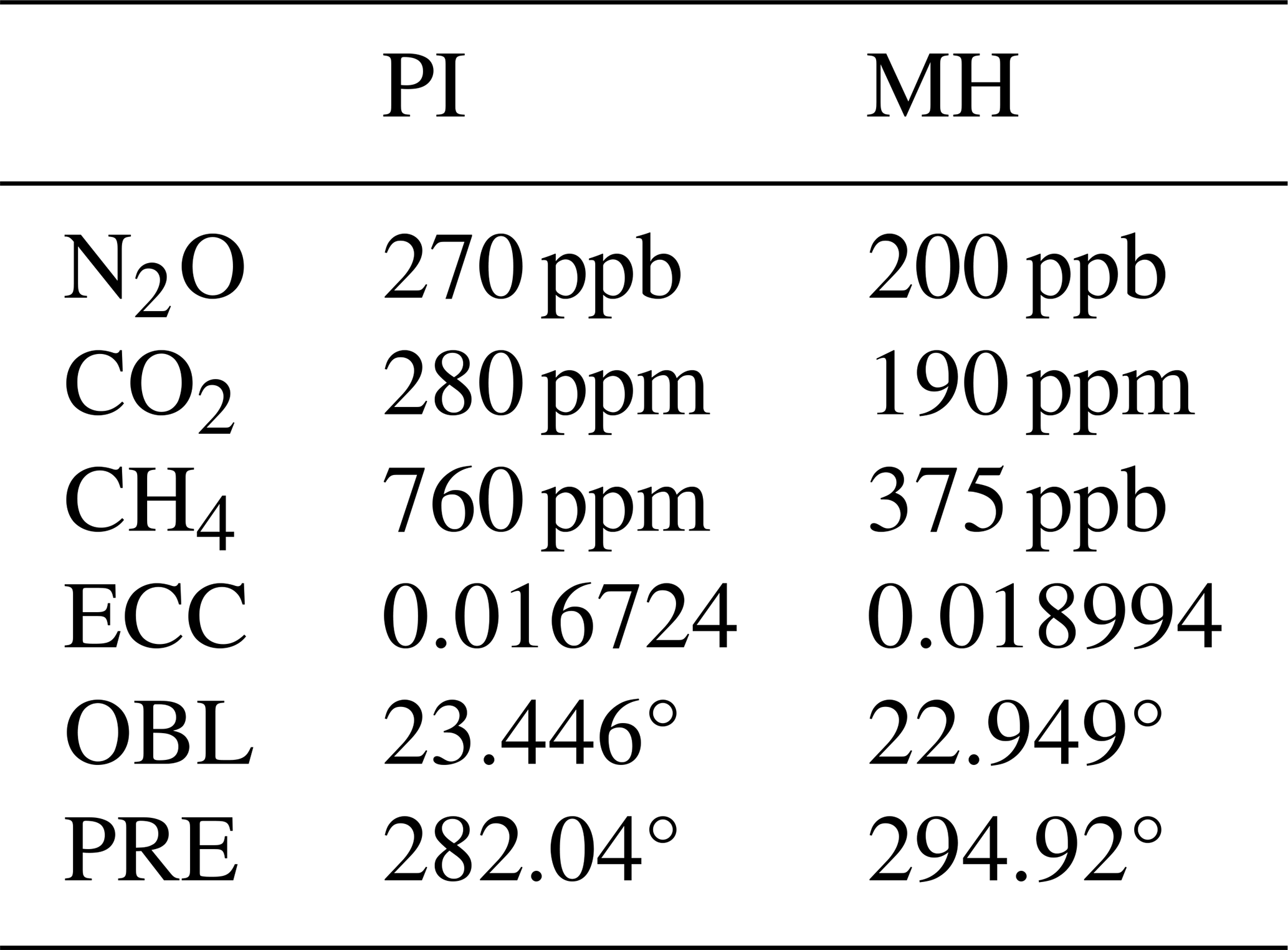
Table 2General description of the WRF model setup of conducted LGM simulations.

Download Print Version | Download XLSX

Having introduced the main features of the WRF simulations in common with Velasquez et al. (2021), we successively describe the main differences with respect to this former study. The initial setup of Velasquez et al. (2021) included a glacier scheme of NOAH-MP, which allowed ice-phase changes in the soil, that was found to be incorrect, producing unrealistic soil temperatures. The here presented simulations use a slab ice scheme of NOAH-MP that does not consider ice-phase changes in the soil, resulting in more realistic soil temperatures than the former option (not shown). Another major improvement with respect to the model version of Velasquez et al. (2021) considered in this study, particularly relevant for the application of WRF to paleoclimate studies, concerns the model representation of changes in the orbital parameters of the Earth on millennial timescales. In fact, while different values of the obliquity of the orbit can be passed directly into the code of the default model version 3.8.1, this is not possible for the different values of the parameters representing changes in the eccentricity of the Earth's orbit around the Sun and in the precession of the equinoxes. For this reason, a FORTRAN subroutine already employed in WRF version 4.1.2 in Ludwig and Hochman (2022) is implemented in the main radiation module of the model to include the full orbital forcing of the LGM experiments. The routine allows for scaling the value of the solar constant depending on the effective position of the Earth on its orbit, taking into account changes in the orbital parameters. It has been developed from a subroutine used in several other paleoclimate studies with the RCM COSMO-CLM (Fallah et al., 2016, 2018; Prömmel et al., 2013; Russo and Cubasch, 2016; Russo et al., 2022) and is based on an original subroutine used in the GCM ECHAM5 (Roeckner et al., 2003), considering basic Kepler laws only and using the long-term series expansions of Laskar et al. (1993). The effect of the implemented subroutine on the seasonal pattern of insolation is here assessed for the coarsest study domain d01. Figure S1 of the Supplement shows the differences in incoming radiation on top of the atmosphere calculated for each day of a year between the LGM and the PI periods, for the default (left) and the new (right) version of the model. The results with the new treatment of orbital parameters (Fig. S1, right) are now in line with the expected seasonal pattern of insolation at the LGM over the study domain (Kageyama et al., 2017), substantially different than the one obtained from the original model version (Fig. S1, left).

2.3 WRF sensitivity experiments

The different CESM simulations with a spatial resolution of 1.25° × 0.9° introduced in Sect. 2.1 are used as initial and boundary conditions to run WRF. A total of five simulations with convection-permitting resolutions are performed with the WRF model for the LGM, each one covering approximately 11 years. For each of these simulations, given the extremely high computational demands of very high-resolution, each period is divided into three sub-periods of different length, between 52 and 40 months and considering the first 4 months as spinup time. In the end, the results of these sub-periods are joined together to retrieve a mean climatology for each of the performed experiments, based on the mean calculated over a total of 10 years. The approach is similar to the one of previous studies such as the one of Velasquez et al. (2020, 2021, 2022). It might not allow for exhaustively assessing the interannual variability in a model over a given period of study, due to the short time frames considered for each experiment. Nevertheless, since the interest of this study is mainly climatological mean values, this represents a good compromise between high demand in computational resources and the length of a signal to be used for building up a climatology. In support of this choice, the results of a 31-year long simulation of Velasquez et al. (2021) are also considered.

Table 3Description of conducted LGM sensitivity experiments with WRF.

Download Print Version | Download XLSX

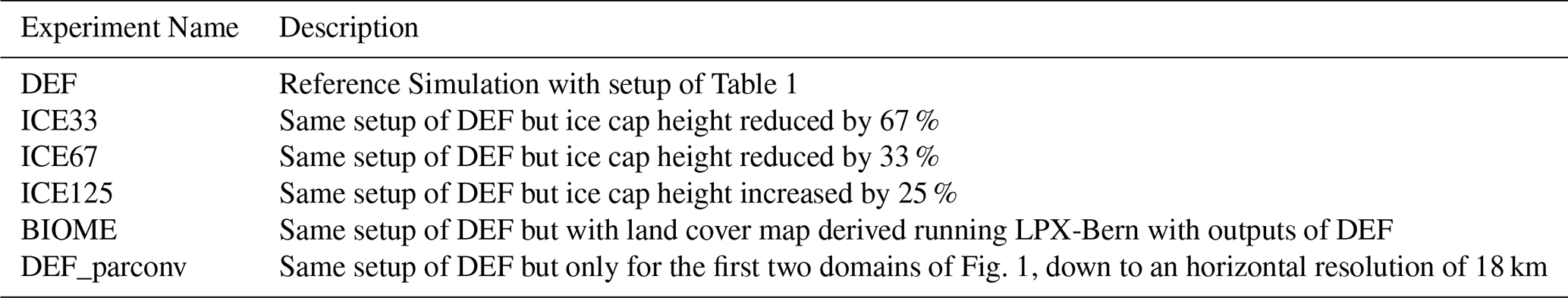
To perform experiments with WRF under LGM conditions, further modifications to the surface boundary conditions are necessary. Changes to land cover, soil composition, ice extent, ice height, and the land–sea mask are applied here to the original present-day WRF datasets. A reference simulation, here referred to as DEF (Table 3), is performed using the outputs from the reference CESM simulation of Buzan et al. (2023) as boundary conditions. For the DEF experiment, the LGM topography is prescribed directly from the dataset of Peltier et al. (2015). In particular, the maximum ice height in the period from 24 and 18 ka as derived from Peltier et al. (2015) is considered in this case. For the Alpine region, in the DEF experiment the ice-cap elevation is derived using the Parallel Ice Sheet Model (PISM, Khroulev and the PISM Authors, 2020) forced by the WRF LGM simulation of Velasquez et al. (2021), and tuned such that the glacial maximum area fits the reconstructed one by Ehlers et al. (2011). The land–sea mask of the DEF simulation is derived from Peltier et al. (2015), also considering the largest extension of ice in between 24 and 18 ka.

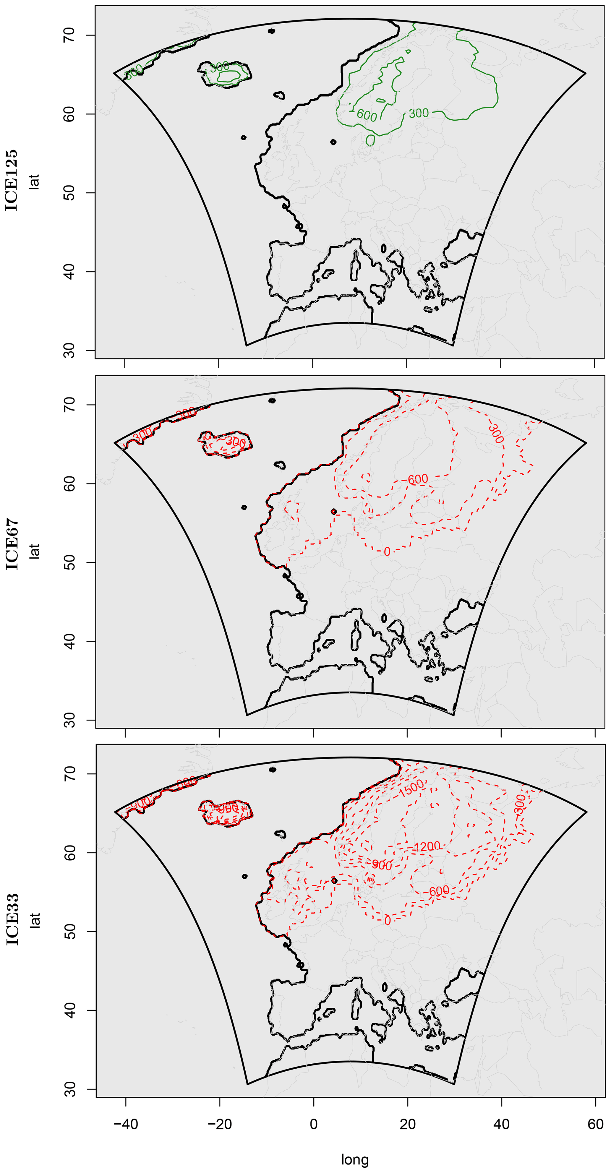
Figure 2Orographic differences in the simulations (from top to bottom) ICE125, ICE67, and ICE33, calculated for the coarser domain of study d01 with respect to the reference simulation DEF. The different contours are drawn at intervals of 300 m. Dotted red contours represent negative values, while continuous green contours represent positive values.

Three additional simulations are conducted using in each case the different boundary data derived from the CESM simulations with perturbed LGM ice height over the higher latitudes of the Northern Hemisphere (see Sect. 2.1). Consistently with the driving data, for these three simulations the height of the northern latitudes ice sheets of the DEF simulation over the considered domain of study is increased by 25 %, and reduced by 67 % and 33 %. These simulations will be referred to, in the following text, respectively, as 125ICE, 67ICE, and 33ICE (Table 3). The orographic differences in each of these simulations with modified ice sheet, calculated for domain d01 with respect to the DEF experiment, are presented in Fig. 2. The most pronounced differences in prescribed topography are evident over the inner part of Scandinavia, with values lower than −1800 m obtained from the comparison between experiments 33ICE and DEF. In all the different cases, the ice-sheet extent (represented as white shadings in Fig. 3) is kept constant.

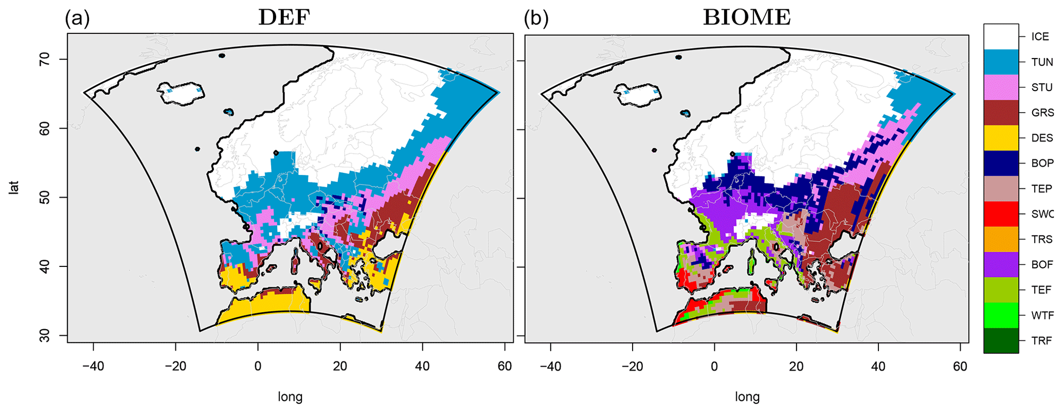
Figure 3LGM land cover and biome classes for the coarser domain of study d01, passed as input to the DEF (a) and BIOME (b) simulations. Besides land ice cover indicated as ICE, all the legend acronyms of the different biome species derived from LPX-Bern are specified in Table 4.

Table 4List of biomes from LPX-Bern (left) and the corresponding ones from MODIS they have been converted to (right).

Download Print Version | Download XLSX

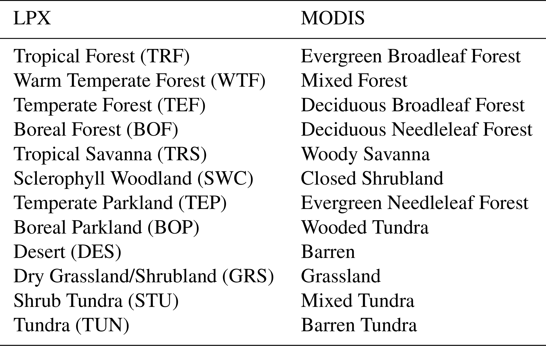
For the LGM land cover, the LGM simulation by Velasquez et al. (2021) is used offline to drive the dynamic vegetation Land surface Processes and eXchanges model of the University of Bern (LPX-Bern v1.4) (Lienert and Joos, 2018; Spahni et al., 2013; Stocker et al., 2013). LPX-Bern features dynamic carbon, water, and nitrogen cycles and vegetation is internally represented by 10 plant functional types (PFTs; eight tree and two herbaceous) competing for resources and adhering to bioclimatic limits. Input variables for LPX-Bern are the fraction of land in a grid cell and monthly values of total precipitation, near-surface temperature, and net downward shortwave radiation at surface. Furthermore, for nitrogen deposition preindustrial values of the forcing product (Tian et al., 2018) closest to the model grid cell are used. LPX-Bern horizontal resolution is adapted to match the horizontal resolution of the respective WRF domains. For using the LGM maps of vegetation derived from LPX-Bern into WRF, the 12 biomes of LPX-Bern need to be translated into one of the 16 classes of WRF (based on the data from the US Geological Survey (USGS)). The selected BIOME correspondence between the two different datasets is presented in Table 3.

All the four simulations introduced above (namely DEF, ICE33, ICE67, and ICE125) use the same vegetation map derived with LPX-Bern from the simulation of Velasquez et al. (2021). Additionally, in order to acknowledge the possible effect of uncertainties in the prescribed land cover, a simulation is performed by driving offline LPX-Bern with the climatological outputs of the DEF simulation. This simulation will be referred to as the BIOME simulation. The DEF and the BIOME experiments are run using the same CESM boundary conditions at 1° × 1° resolution. A map of the two different land cover datasets used for the conducted experiments is presented in Fig. 3. For a large part of the domain there are noticeable differences in vegetation, both on a continental and local scale. The two datasets seem to correspond only over a remote part of northeastern Europe. For this reason, the designed experiments are likely to provide important information on the role of uncertainty related to the use of a different land cover in RCM simulations of European climate at the LGM. Present-day soil categories are used for all the LGM simulations, with some modifications: all the soil layers corresponding to a point covered by glaciers are set to ice. Consistently, for a given grid box, the same soil category of the upper soil layer is used for all soil levels at different depths.

In order to conduct a more quantitative evaluation of WRF against the pollen-based reconstructions taking into account different model uncertainties, the five experiments introduced above (i.e., DEF, ICE33, ICE67, ICE125, and BIOME) are considered together as an ensemble of simulations. Here, as model uncertainty, we consider the range of outputs that is obtained using the same model but applying changes to the model chain setup inherent to land cover and ice height.

Finally, in addition to the already described simulations, an experiment with the same setup of the DEF simulation but using only two nested domains, D01 and D02, down to a spatial resolution of 18 km and with the convection parameterization switched on (i.e., convection is not explicitly solved), is performed. This experiment is indicated as DEF_parconv in Table 3 and is conducted with the goal of better assessing the role of convection-permitting simulations for the representation of the European LGM climate.

2.4 Proxy reconstructions dataset

The model simulations are evaluated against a new pollen-based reconstruction of LGM seasonal and annual temperature and precipitation by Davis et al. (2022). This reconstruction is based on pollen data from 63 pollen records that were selected for the quality of their dating control over the LGM period (21 ka cal ±2 kyr). Records were excluded if they fell within category 7 (“poor”) of the 1–7 COHMAP scale of chronological quality based on the proximity of dates to the LGM time slice. Only absolute dating methods (e.g., radiometric dating such as radiocarbon) were considered, and relative dates based on pollen correlation were excluded. The record selection process, therefore, excluded many of the pollen records used in previous studies, reflecting the generally poor quality of the dating control in LGM pollen records, including 10 of the 18 records used in the PMIP benchmarking dataset (Bartlein et al., 2011). The reconstruction itself uses a standard modern analogue technique (MAT) that finds the best six analogues amongst a dataset of over 8000 modern pollen samples from the Eurasian Modern Pollen Database (Davis et al., 2020). The MAT method has been used for previous LGM pollen–climate reconstructions (Peyron et al., 1998) but it has not been known how much the method may be influenced during the LGM by problems such as having no modern analogue vegetation (and climate), as well as changing plant physiological responses to climate associated with lower atmospheric CO₂. For this reason, the method was evaluated against a previous pollen–climate reconstruction based on inverse modeling (Wu et al., 2007), which is designed to account for many of these problems, as well as a chironomid-based reconstruction (Samartin et al., 2016). The result of this evaluation showed little difference between the MAT reconstruction and these other methods, indicating that the MAT method is reliable for this time period and location. This can be attributed in part to advances in the size and spatial coverage of the modern pollen training set, which is an order of magnitude larger than those used in previous MAT reconstructions, permitting good vegetation analogues (chord distance <0.3, Huntley, 1990) to be found for all fossil pollen samples. Importantly, the uncertainty estimates of the considered pollen-based reconstructions are considered in their comparison against the results of the presented model simulations.

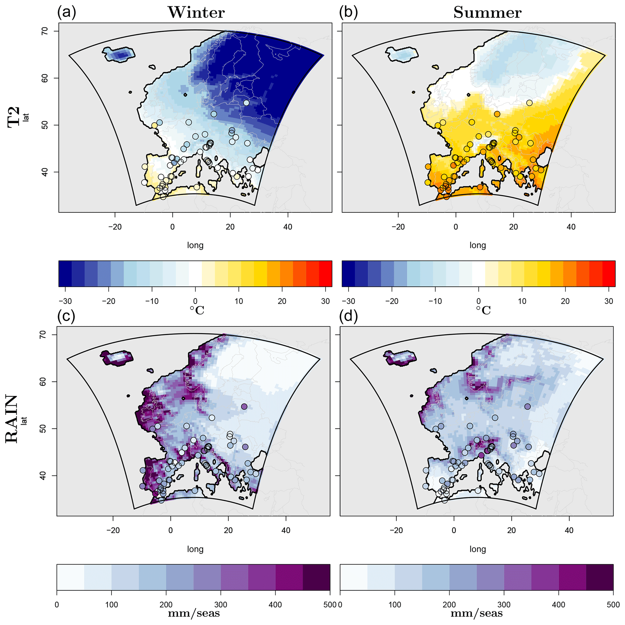
Figure 4LGM winter (a, c) and summer (b, d) climatological values of mean near-surface temperature (a, b) and precipitation (c, d) as derived from the reference WRF LGM simulation, for the domain d01 of Fig. 1, at coarser resolution. The circles represent the values as derived from pollen-based reconstructions.

3.1 Comparison of the reference simulation against pollen-based reconstructions

In Fig. 4 we present the mean climatologies of winter and summer temperatures and precipitation of the DEF LGM simulation over the coarsest domain of the study, together with the corresponding values derived from the pollen-based reconstructions. Winter temperatures below 0 °C characterize almost the entire domain for the DEF experiment, except for a few points over southern Spain and northwestern Africa. Particularly cold simulated temperatures are evident in winter over the northeastern part of Europe, with values generally below −25 °C. Temperatures remain lower than 0 °C in the model in summer over north and northeastern Europe, over areas largely covered by glaciers. Simulated temperatures rarely exceed a mean value of 20 °C in summer, only over specific areas of southern Europe and northern Africa. The values of the pollen-based reconstructions, displayed in Fig. 4 as filled circles, show a similar behavior, even though their coverage is mainly limited to central and southern Europe. In winter, the pollen data are also characterized by a northeast-to-southwest gradient in temperatures, with values consistent with the ones of the WRF DEF experiment. In summer, reconstructed temperatures are similar to the ones simulated by WRF for the entire domain, presenting in particular a similar north-to-south gradient. The simulated precipitation pattern in winter is characterized by high values in the western areas of the domain (Fig. 4, lower row), for which moisture advection from the Atlantic Ocean plays a major role (Beghin et al., 2016; Ulbrich et al., 1999), up to seasonal values of 500 mm/season in some cases. In summer, drier conditions are evident over almost the entire domain, except for few areas with complex topography such as part of the Alps and western Scandinavia, where precipitation exceeds 300 mm/season. The pollen-based reconstructions show a slightly different picture compared to the DEF simulation for precipitation in winter. While the western coastal areas are wetter than eastern Europe according to the pollen, pronounced dry conditions are evident over the central part of the domain, particularly at the northern edges of the Alps. Additionally, the range of values of winter precipitation derived from the pollen-based reconstructions is generally narrower than in the case of the DEF simulation, with maximum values rarely exceeding 250 mm/season. For summer precipitation, on the other hand, there is a better agreement between the simulated data and proxy reconstructions than in winter, except for specific areas, such as again around the Alps. In summer, the simulated values of precipitation are in the same range as the climate reconstructions.

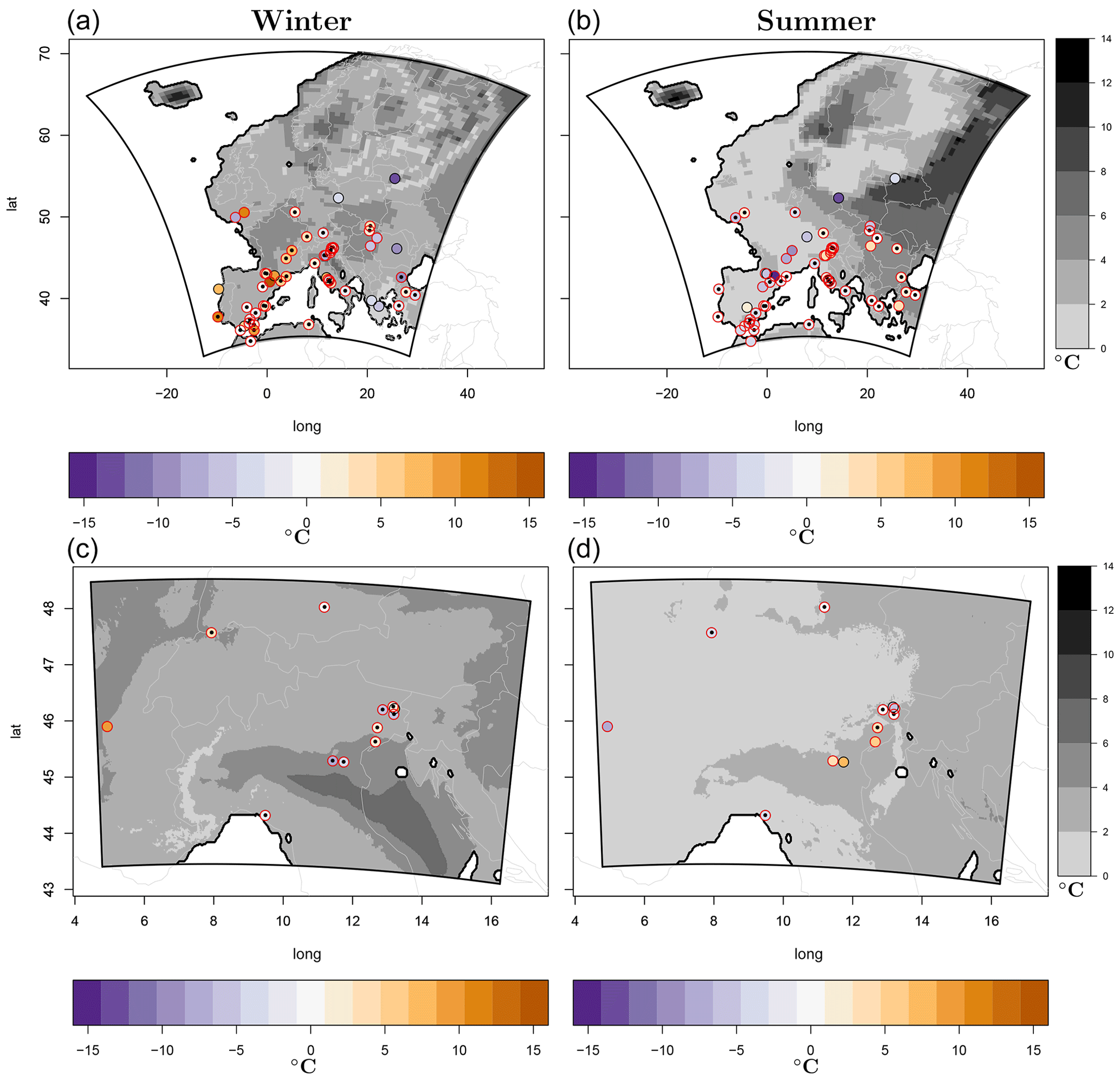
Figure 5Maps for the bias of winter (a, c) and summer (b, d) temperatures calculated between the WRF reference simulation and the pollen-based reconstructions. Upper row (a, b) shows the results for the coarser-resolution domain d01, while the bottom row (c, d) presents the same analysis for the higher-resolution domain d04. The colored circles show the biases calculated between the two datasets. In the case of the bias being smaller than 1 standard deviation of the reconstructions, a black dot is added at the center of the circle. Considering then the five-member ensemble, in the case of the bias of at least one of these members against the reconstructions being smaller than 1 standard deviation of the latter, then the circle is highlighted in red. Finally, the gray scale represents the maximum differences for each point of the domains, between the different members of the ensemble.

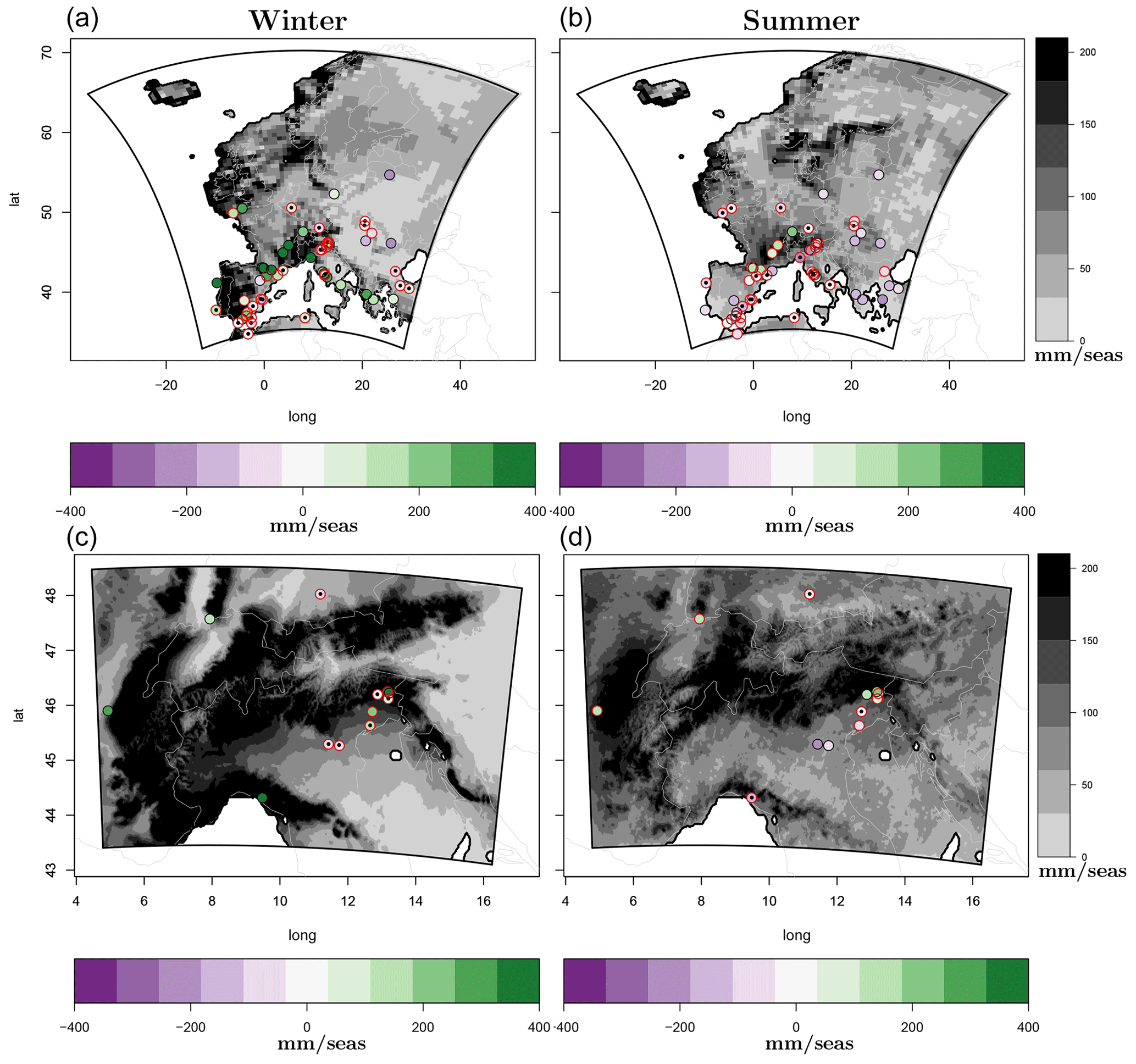
Figure 6Maps for the bias of winter (a, c) and summer (b, d) seasonal precipitation calculated between the WRF reference simulation and the pollen-based reconstructions. Upper row (a, b) shows the results for the coarser-resolution domain d01, while the bottom row (c, d) presents the same analysis for the higher-resolution domain d04. The colored circles show the biases calculated between the two datasets. In the case of the bias being smaller than 1 standard deviation of the reconstructions, a black dot is added at the center of the circle. Considering then the five-member ensemble, in the case of the bias of at least one of these members against the reconstructions being smaller than 1 standard deviation of the latter, then the circle is highlighted in red. Finally, the gray scale represents the maximum differences for each point of the domains, between the different members of the ensemble.

3.2 Consideration of different model uncertainties

A more quantitative assessment of the differences in seasonal values of temperature and precipitation between the DEF WRF simulation and the pollen-based reconstructions is provided in Figs. 5 and 6, respectively. In these figures, the temperature and precipitation derived from the additional WRF simulations BIOME, 33ICE, 67ICE, and 125ICE of Table 3 (forming, together with the DEF simulation, a five-member ensemble) are also considered. The comparison between the pollen-based reconstructions and the model outputs is additionally conducted on both the coarse-resolution domain, and the inner domain d04 of Fig. 1 in this case. A circle with the values of the differences between the reference simulation DEF and the pollen-based reconstructions is drawn for the proxy locations. If the bias of the reference simulation DEF lies within 1 standard deviation of the uncertainty values of the pollen-based reconstructions, then a black dot is added at the center of a given circle. Successively, if at least one of the five-member ensemble lies within 1 standard deviation of the pollen values, then the circle is highlighted in red. Finally, the maximum absolute differences in the considered variables calculated between the different ensemble members are plotted for each point of the domain on a gray scale in order to provide an assessment of the ensemble spread and model uncertainty.

Figure 5 confirms that, for both winter and summer, there is a very good agreement in temperatures between the performed simulations and the values derived from the proxies. The consideration of the different simulations with the applied changes in the model configuration allow for obtaining results that are very close to the evidence of the proxies for almost the entire points of the domain, in both seasons and for both considered variables. For winter temperature, the bias of the reference (DEF) exceeds in very few cases an absolute value of 5 °C. Interestingly, despite the large changes in the configuration of the different ensemble members, their results in terms of winter temperature are relatively close for almost the entire domain of study (see also Fig. S2). Differences between the different ensemble members larger than 4 °C are evident for winter temperature mainly over the northeastern part of the domain and Iceland, with values of the different ensemble members spreading here over a range of more than 10 °C. For summer, again, the mean model temperatures are very close to the values of the pollen-based reconstructions over the entire domain (Fig. 5, right column). The DEF simulation, in particular, shows a small bias against the proxies over the entire domain, with values rarely exceeding 4 °C and well within the range of the pollen uncertainty. The main exceptions are some points over the area of present-day France, for which a closer agreement is reached only when considering other members of the ensemble. In summer, more notable and spatially heterogeneous differences in temperatures are evident between the different ensemble members than in winter. In particular, large differences, of up to 14 °C, are found between the different experiments for areas at the border of glaciers over Scandinavia and Iceland, mainly due to a reduction in the height of glaciers over these regions (Fig. S3).

Analyses for the inner Alpine domain (Fig. 5, bottom row) confirm an overall good match between temperatures derived from the performed simulations and the pollen-based reconstructions, for both summer and winter. In this case, the main differences between the different ensemble members are evident in winter over the Po valley, exceeding in some cases 6 °C. Just two points of the pollen reconstructions, in summer, have temperature values outside the range of the ensemble members for the inner domain of study. This gives high confidence on the use of the presented results for the study of the LGM climate of the area.

For precipitation (Fig. 6), the agreement between model simulations and proxy reconstructions is not as good as in the case of temperature. In winter, the model seems to be generally too wet, in particular over the northern Iberian Peninsula, present-day France, the Alps, and continental areas of present-day Greece and Turkey, with seasonal values of precipitation exceeding the ones derived from pollen-based reconstructions by more than 300 mm/season. For these areas, none of the performed simulations gets significantly closer to the range of values of the proxies, also when taking into account pollen uncertainties. It is important to note here that most of the locations for which the model presents the largest positive biases in winter precipitation are at the boarder of mountainous areas covered with glaciers, such as the Alps and part of the Pyrenees. This positive bias could partly be related to uncertainties in the extent or height of the prescribed glaciers, not properly resolved at the scales characteristic of the considered pollen data. This is confirmed by the fact that the bias for the two points northwest of the Alps is reduced when considering the model results over the Alpine region at an horizontal resolution of 2 km (Fig. 6, bottom row). In winter, the areas for which the DEF simulation presents higher values of precipitation, i.e., western Europe (Fig. 4, lower row), are the same as those for which higher differences in the ensemble members are evident, exceeding in most of these areas 150 mm/season. These pronounced differences between the different ensemble members are mainly dictated by the experiments with changes in the height of glaciers (Fig. S4). A similar overlapping of the largest differences in the ensemble members over regions presenting the highest values of precipitation in the DEF simulation is also evident in summer. In this case though, there is a better agreement between the results of the performed simulations and the pollen-based reconstructions, although the model seems to be generally drier, in particular over the Balkans, where the differences against the pollen-based reconstructions are in some cases below −200 mm/season. Notable in this case is that changes in land cover seem to be very important for the representation of summer precipitation over the Mediterranean region, in particular over the Balkans (Fig. S5), where the BIOME simulation produces significant changes with respect to the DEF experiment.

For the inner domain of study there is also a relatively good agreement between the proposed simulations and the pollen-based reconstructions in terms of precipitation, for both seasons, but this is again worse than in the case of temperature (Fig. 5, lower row), at least when considering the number of points for which the simulations lie within the pollen uncertainty. Three important points need to be mentioned in the case of precipitation for the inner domain of study. Firstly, the differences between the different ensemble members are considerable over all of the Alpine range, in both winter and summer, with values extensively exceeding 200 mm/season. This confirms again the relevance of the considered sources of uncertainty in the model for the investigation of the LGM climate of the region. Secondly, even though the simulations are out of the range of the considered pollen-based reconstructions over some points in one season, they get closer in the other. This indicates that some of the results, even if not perfectly matching the values of the proxies, are not completely off. Thirdly, a point also valid for the rest of the domain is that the pollen reconstructions are trained with present-day observations, and studies show that even observations nowadays tend to underestimate precipitation in particular areas characterized by complex terrain (Fu, 1996; Frei and Schär, 1998; Frei et al., 2003).

Finally, to confirm that the differences between the different ensemble members are robust and not simply an effect of the selection of a relatively short simulation period of 10 years, from which the climatological values are obtained, we have also calculated the maximum differences in the climatological values of 20 different periods of 10 years derived from the 31-year long simulation of Velasquez et al. (2021), for summer temperatures. The results, as illustrated in Fig. S6, indicate that the spread of this set of experiments is negligible compared to the one obtained when comparing the different realizations of our five-member ensemble.

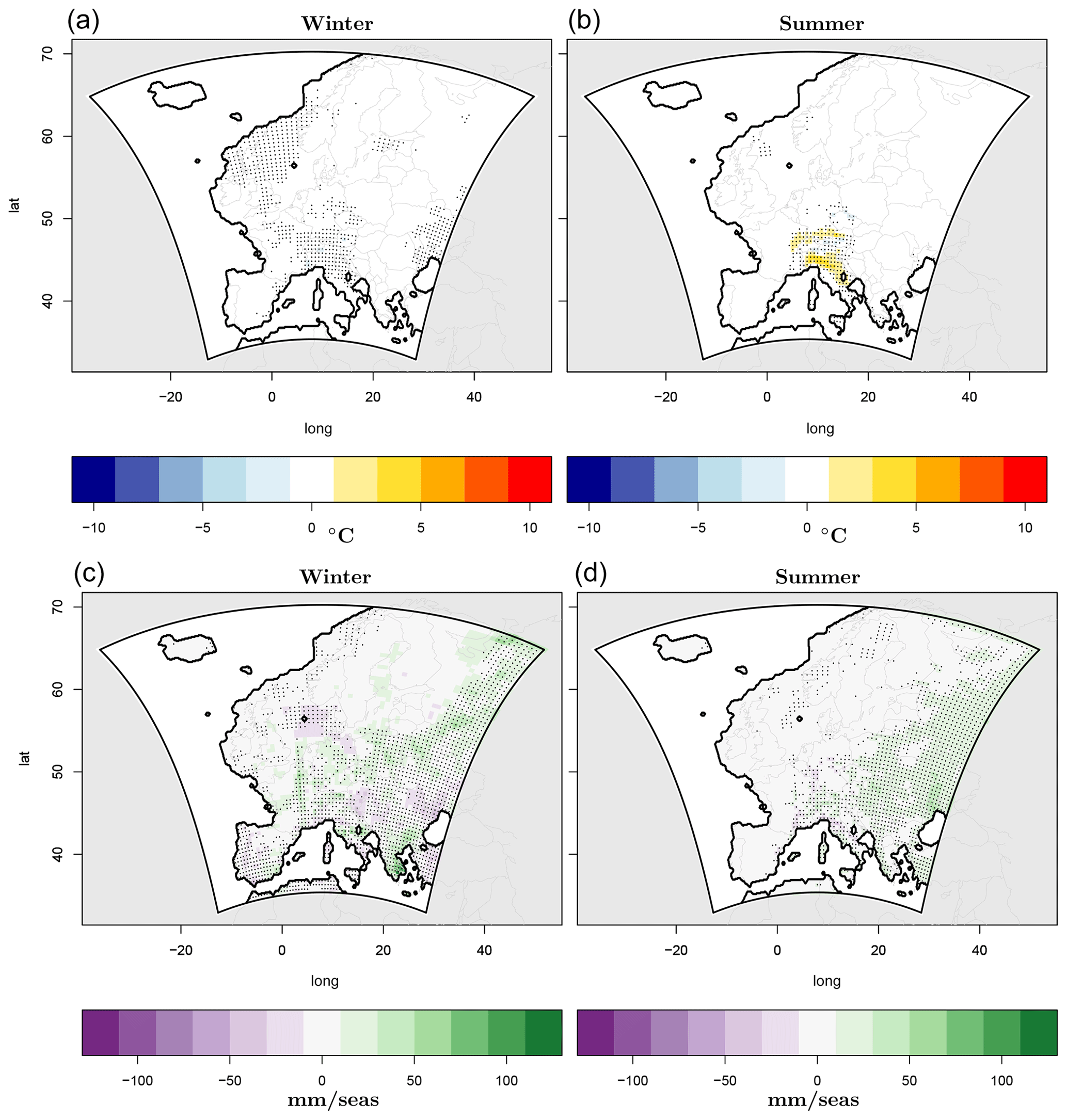
Figure 7Bias in winter (a, c) and summer (b, d) values of temperatures (a, b) and precipitation (c, d) calculated for the coarser-resolution domain d01, between the reference simulation and the one with only two nested domains, down to 18 km. The dots in each of the panels represent the points for which the values differ significantly, at a significance level of 0.05, according to the results of a KS significance test.

3.3 Considerations on the role of convection-resolving resolutions

In Fig. 7 the differences in the mean seasonal values of temperature and precipitation between the reference DEF simulation and the DEF_parconv experiment are calculated for each grid box of the outer domain d01. The main goal of such an analysis is to assess whether the explicit representation of convection over the inner part of the domain has a relevant impact on the simulated variables at both the local and continental scale, with respect to a simulation exclusively using a parameterized representation of convection over all the domain. In Fig. 7, for each grid-box where the daily mean anomalies of the considered variable and season can be considered significantly different according to the results of a Kolmogorov–Smirnov (KS) significance test at a significance level of 0.05, a dot is plotted.

Results show that for the Alpine region, the effects of higher resolution and the explicit representation of convection are significant, for both variables and seasons. For precipitation, in particular, the effects of the convection-permitting simulation are seen not only over the inner domains but also over the entire domain of study, presenting significant differences between the two simulations. These differences are in some cases of the same order of magnitude as the differences between the different sensitivity tests conducted by perturbing the glaciers ice height and extension (see Supplement, Fig. S2) and considering considerably different boundaries discussed in Sect. 3.2. Therefore, the consideration of convection-permitting resolutions for the simulation of European LGM climate has a significant impact on the results, comparable to the effect of other relevant sources of uncertainty, not only at a local scale but over the entire European domain.