2.1 ECHAM6-wiso

ECHAM6 (Stevens et al., 2013) is the sixth generation of the atmospheric general circulation model ECHAM, developed at the Max Planck Institute for Meteorology. It consists of a dry spectral-transform dynamical core, a transport model for scalar quantities other than temperature and surface pressure, a suite of physical parameterizations for the representation of diabatic processes, and boundary datasets for externalized parameters (trace gas and aerosol distributions, land surface properties, etc.). ECHAM6 forms the atmospheric component of the fully coupled Earth system model MPI–ESM (Giorgetta et al., 2013; Mauritsen et al., 2019). The implementation of the water isotopes in ECHAM6 as part of MPI–ESM has been described and evaluated in detail by Cauquoin et al. (2019b), and this model version has been labeled ECHAM6-wiso. At a later stage, Cauquoin and Werner (2021) updated the water isotope module of ECHAM6-wiso in several respects. The supersaturation has been slightly retuned, the kinetic fractionation factors for the evaporation over the ocean are now assumed to be independent of wind speed, and the isotopic content of snow on sea ice is taken into account for sublimation processes in sea-ice-covered regions. The latter leads to a stronger depletion of surface water vapor over such sea-ice-covered areas (while the surface temperature remains the same). As a consequence, this change is expected to contribute to a steeper temporal isotope–temperature slope over sea-ice-covered areas.

2.2 Sea surface temperature and sea ice extent boundary conditions for LGM conditions

2.2.1 SST

The Tierney et al. (2020a) SST reconstruction has a larger and more homogeneous cooling than GLOMAP, except for the high southern latitudes at which the Pacific sector cools more than the Atlantic sector (Fig. 1). On the other hand, the LGM cooling in the northern North Atlantic Ocean is stronger in GLOMAP than in the Tierney et al. (2020a) reconstruction (−5.4 and −4.8 ^∘C, respectively, see Table 4 in Paul et al., 2021). These differences between the two SST reconstructions are due to the use of different proxy datasets for the reconstructions (geochemical proxies only for Tierney et al., 2020a, MARGO dataset for GLOMAP) and the methods applied to produce SST gridded maps from scattered observations (see Sect. 1). For their offline data assimilation technique, Tierney et al. (2020a) used results from the coupled climate model iCESM1.2, which shows one of the largest coolings among the PMIP4 models (Fig. 1b of Kageyama et al., 2021). In addition to these two reconstructions, we used SST and sea ice extent outputs from a MIROC 4m LGM simulation (Obase and Abe-Ouchi, 2019) with oscillating AMOC strength. The global LGM cooling is between −2.3 and −2.7 ^∘C according to the considered simulations (Fig. 1), i.e., higher than GLOMAP and lower than the Tierney et al. (2020a) reconstruction. The main specificity of MIROC 4m LGM SST is a very strong cooling in the North Atlantic (more than 10 ^∘C, Fig. 1) and more uniform temperature anomalies between −2 and −4 ^∘C in the other areas, including off the coast of Greenland. We extracted the MIROC 4m SST outputs, averaged over a 100-year period, at two different times of the LGM simulation depending on the AMOC strength: during a weak AMOC phase (average AMOC index was equal to 8.44 Sv) and a strong AMOC phase (19.95 Sv). A weaker AMOC during LGM implies larger cooling in the North Atlantic (Fig. 1) and more extended sea ice (Fig. 2), with less cooling in the Southern Ocean. The strong AMOC phase period in the MIROC 4m simulation was selected in the middle of the AMOC peak (Fig. S1 in the Supplement). Therefore, the values of MIROC 4m average near-surface air temperature in Antarctica are very similar regardless of the selected AMOC phase. For example, MIROC 4m simulates LGM temperature of −41.87 and −41.75 ^∘C at the WAIS Divide Ice Core (WDC) station for a strong and weak AMOC phase, respectively. A similar pattern is found for the eastern part of the continent (−56.80 and −56.50 ^∘C at Dome Fuji for a strong and weak AMOC phase, respectively).

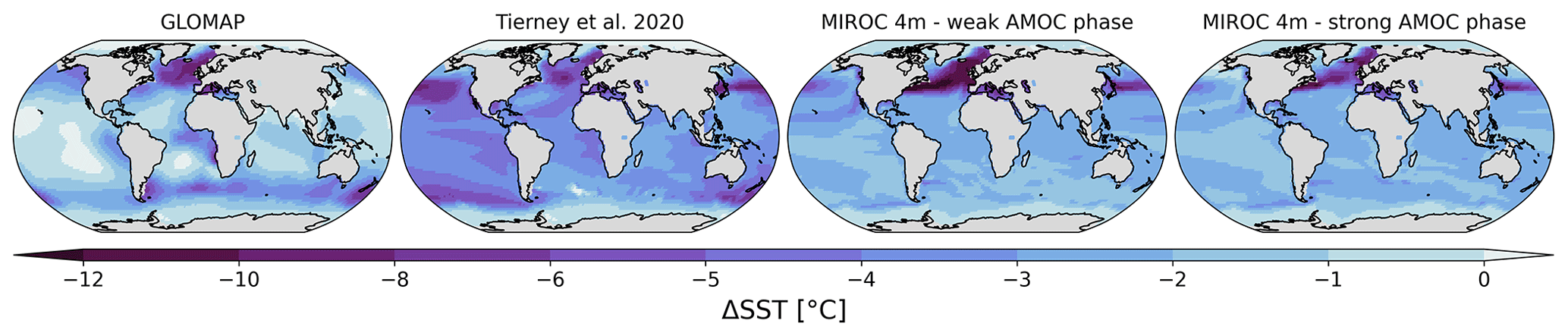
Figure 1LGM–PI sea surface temperature changes used as boundary conditions for ECHAM6-wiso simulations. From left to right: GLOMAP (Paul et al., 2021), Tierney et al. (2020a), MIROC 4m with weak LGM AMOC phase, and MIROC 4m with strong LGM AMOC phase. Anomalies are expressed relative to Atmospheric Model Intercomparison Project mean SST over the period 1870 to 1899.

2.2.2 Sea ice extent

Maps of the averaged sea ice area fraction used as boundary forcings for ECHAM6-wiso are shown in Fig. 2. The PI AMIP and LGM GLOMAP sea ice cover is higher around Antarctica compared to MIROC 4m ones, with a further extent in the Southern Ocean, especially in the Atlantic sector. On the other hand, sea ice is more extensive in the Northern Hemisphere for MIROC 4m in the weak AMOC phase. For the stronger AMOC case, a decline of the sea ice in the Northern Hemisphere is seen, accompanied by weaker cooling (see Sect. 2.2.1). In its parameterization, MIROC 4m uses a threshold of 95 % for the sea ice fraction to allow sub-grid “sea ice leads”. This threshold is not rigid, but it is difficult to exceed sea ice concentrations of 95 % unless there is significant convergence of sea ice. Consequently, while the sea ice is, on average, more extensive in the north in MIROC 4m for the weak AMOC phase compared to the GLOMAP reconstruction, the sea ice area fraction in grid cells near coastal areas like Greenland is lower in MIROC 4m than in GLOMAP (95 %–98 % against 100 %, respectively).

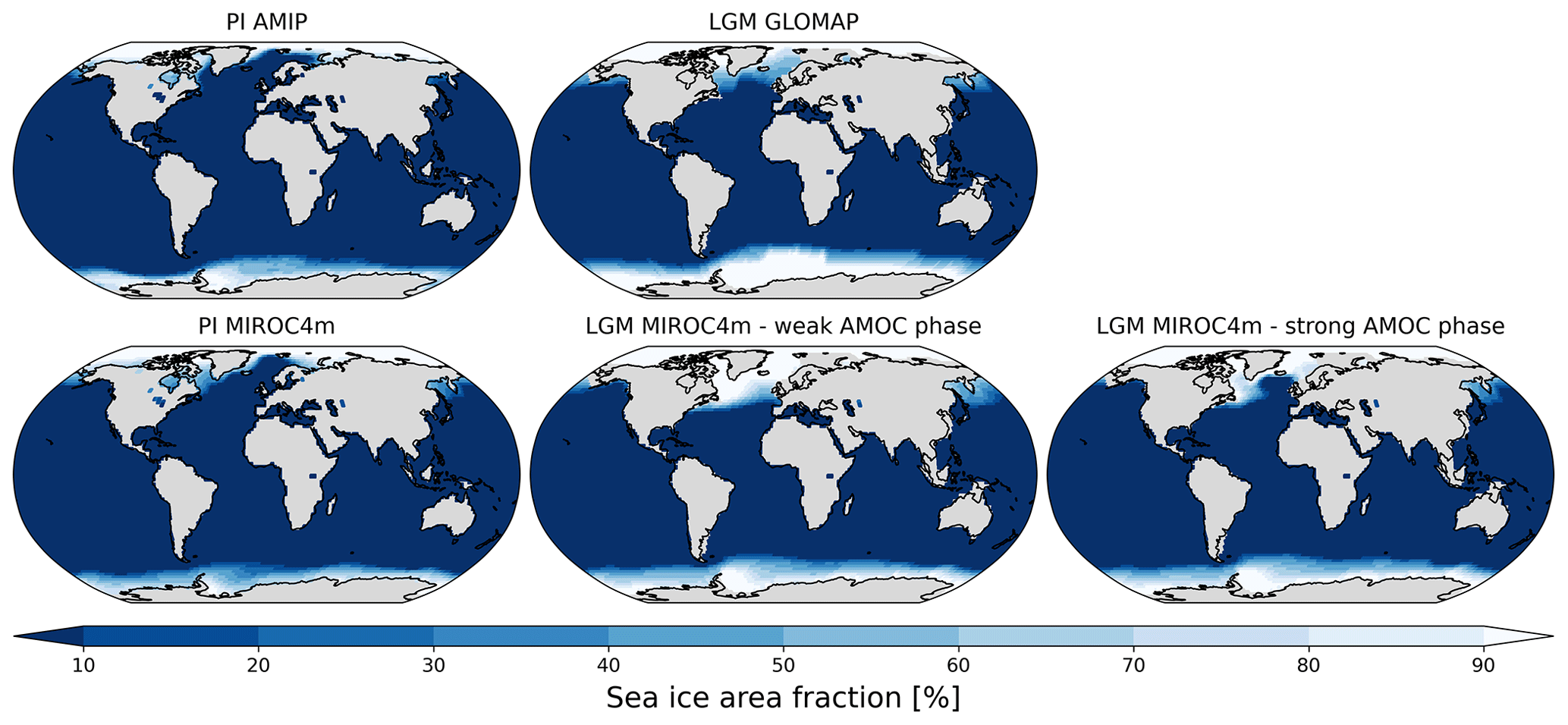
Figure 2LGM and PI sea ice area fractions used as boundary conditions for ECHAM6-wiso simulations.

2.3 Model setup and experiments

We performed an ensemble of LGM simulations with ECHAM6-wiso, forced with different combinations of SST and sea ice boundary forcings presented in Sect. 2.2. All our PI and LGM simulations are designed with respect to the PMIP4 protocol (e.g., greenhouse gas and orbital conditions). The LGM SST boundary fields are expressed relative to the Atmospheric Model Intercomparison Project (AMIP, Eyring et al., 2016) mean SST (averaged over the period 1870 to 1899) used for the preindustrial simulations (Table 1). The GLOMAP reconstruction has the advantage of providing a monthly climatology of LGM SST and sea ice extent, while only annual mean SST is available from the reconstruction by Tierney et al. (2020a), without a sea ice map distribution. So, the Tierney et al. (2020a) LGM SST for ECHAM6-wiso was produced by taking the annual mean SST anomaly from Tierney et al. (2020a) and adopting the monthly climatology temperature variability from GLOMAP. Since we also used GLOMAP sea ice extent data in this case, the SST was adjusted slightly to maintain consistency (e.g., SST set to freezing temperature where there is sea ice). In order to investigate the impact of sea ice extent on our isotope results and the related isotope–temperature slopes for LGM-to-PI climate change, we used LGM SST outputs from MIROC 4m simulations combined with sea ice extent data from the same MIROC 4m simulations or from the GLOMAP dataset. To evaluate the LGM–PI anomalies, we performed several PI simulations with different sea ice boundary conditions depending on the setup of LGM experiments using climatological monthly mean sea ice area fractions from AMIP or MIROC 4m coupled simulations (Table 1). The prescribed LGM ice sheet is GLAC-1D (Tarasov and Peltier, 2002; Tarasov et al., 2012, 2014; Abe-Ouchi et al., 2013; Briggs et al., 2014) for all LGM simulations. As with SST and sea ice distribution, mean δ¹⁸O of surface seawater needs to be prescribed. For the PI simulations, we used the δ¹⁸O reconstruction from the global gridded dataset of LeGrande and Schmidt (2006). As no equivalent dataset of the δ²H composition of seawater exists, the deuterium isotopic composition of the seawater in any grid cell has been set equal to the related δ¹⁸O composition, multiplied by a factor of 8, in accordance with the observed relation for meteoric water on a global scale (Craig, 1961). As in Werner et al. (2018), a prescribed glacial seawater enrichment of +1 ‰ and +8 ‰ is assumed for δ¹⁸O and δ²H in the LGM simulations, respectively. The PI and LGM simulations were run for 60 and 120 model years, respectively, and we used the last 30 model years for our analyses. The simulation characteristics are summarized in Table 1. Two additional sensitivity simulations have been performed to evaluate the impacts of lower MIROC 4m sea ice area fraction in coastal grid cells (Sect. 2.2.2) and the consideration of the isotopic composition of snow on sea ice in ECHAM6-wiso (Sect. 2.1) on the modeled δ¹⁸O_p–temperature temporal slopes between LGM and PI (see Supplement Sect. S1). Also, an LGM simulation using the PMIP3 ice sheet reconstruction instead of GLAC-1D (see Fig. 3b and d of Werner et al., 2018, respectively) has been performed to evaluate the impact of ice sheet topography on the isotopically enriched bias in Antarctica (Sect. S1).

Table 1Characteristics of the ECHAM6-wiso simulations in the present study.

Download Print Version | Download XLSX

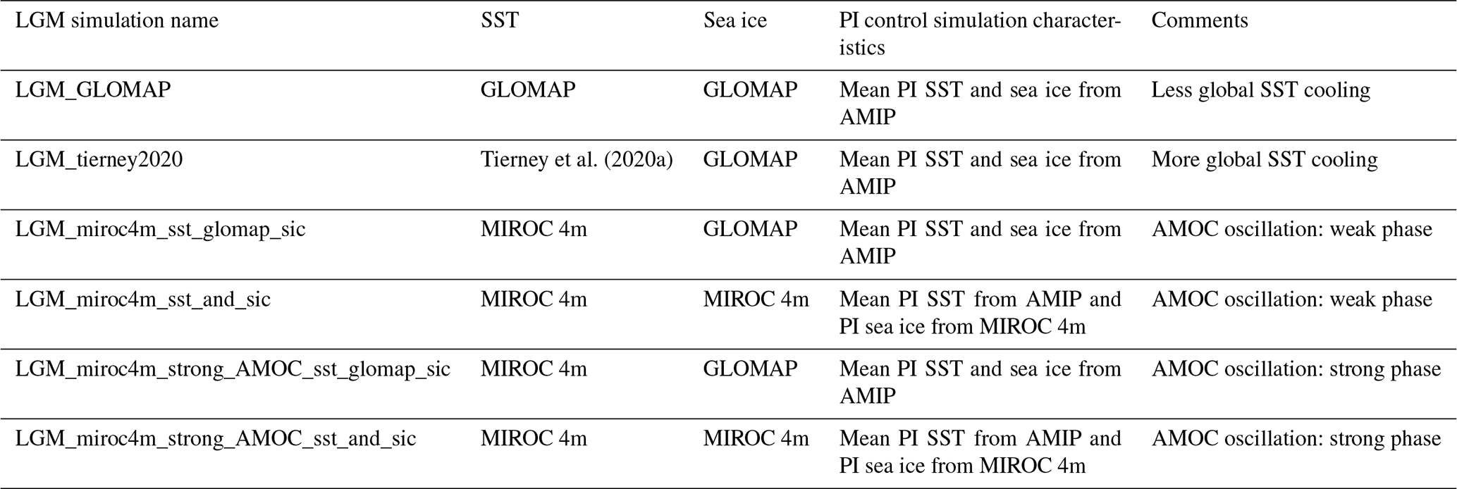
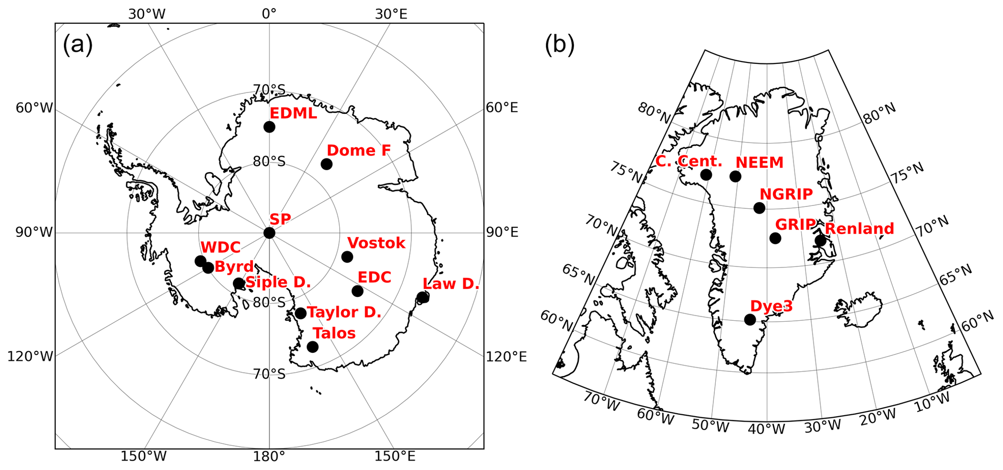
Figure 3Location of polar ice core sites in Antarctica (a) and Greenland (b).

2.4 Observational data

To evaluate the modeled δ¹⁸O of precipitation and snow values at ice core stations, we use a selection of 6 Greenland and 11 Antarctic ice cores for the preindustrial and LGM climates (Fig. 3). The observed δ¹⁸O values were defined as averages over the last 200 years for the preindustrial period and in the 21±1 ka period for the LGM. We also use LGM–PI δ¹⁸O anomalies from five (sub)tropical ice cores that are reported in Table 2 of Risi et al. (2010). The ice core data used in this study are summarized in Table 2. Similarly, we use temperature reconstructions based on borehole reconstructions or δ¹⁵N for seven Antarctic cores and one Greenland ice core (Buizert et al., 2021; Dahl-Jensen et al., 1998) to evaluate the air surface temperatures near the surface, as modeled by ECHAM6-wiso. In order to mitigate the seasonal bias when comparing observed δ¹⁸O from snow in ice cores with modeled δ¹⁸O of precipitation or deposited snow, the modeled δ values are calculated as a precipitation-weighted (or snow-weighted) mean with respect to the V-SMOW scale. For the evaluation of modeled δ¹⁸O of precipitation at a global spatial scale, we extracted 14 entities from the SISALv2 speleothem dataset (Comas-Bru et al., 2020) for which both PI and LGM δ¹⁸O values of calcite or aragonite are available (see Sect. S2 for the details).

Table 2Selected ice core records and their geographical coordinates, reported PI values of δ¹⁸O, changes in δ¹⁸O between LGM and PI, and modeled range of Δδ¹⁸O among our simulations reported in Table 1.

References: ^a Steig et al. (2021). ^b Risi et al. (2010). ^c WAIS Divide project members (2013). ^d Kawamura et al. (2007). ^e Stenni et al. (2010). ^f Landais et al. (2015). ^g Steig et al. (2000). ^h Stenni et al. (2011). ⁱ Blunier and Brook (2001). ^j Vinther et al. (2009). ^k Vinther et al. (2006). ^l North Greenland Ice Core project members (2004). ^m Guillevic et al. (2013). ⁿ Schüpbach et al. (2018).

Download Print Version | Download XLSX

3.1 Evaluation of ECHAM6-wiso under LGM conditions

We evaluate the global distribution of δ¹⁸O of precipitation (δ¹⁸O_p) changes between LGM and PI (Δδ¹⁸O_p) from our different ECHAM6-wiso simulations. Figure 4 shows the comparison of modeled δ¹⁸O_p anomalies with isotope measurements from ice cores and speleothems for the simulation LGM_miroc4m_sst_and_sic (i.e., SST and sea ice boundary conditions from the MIROC 4m simulation in a weak AMOC phase). Well-known patterns of global Δδ¹⁸O_p distribution are found in ECHAM6-wiso, like the negative anomalies across Canada, Greenland, and northern Europe due to the presence of glaciers in these areas during LGM period (Fig. 4c). Generally, negative δ¹⁸O_p anomalies are also simulated over Antarctica and the Southern Ocean, where the LGM cooling is stronger compared to lower southern latitudes (Fig. 4a). In the middle to low latitudes, Δδ¹⁸O_p is mainly controlled by precipitation anomalies (Fig. 4b). For example, lower modeled precipitation in the Amazonian area, over parts of Southeast Asia, and in the western Pacific Ocean during the LGM leads to positive modeled δ¹⁸O_p anomalies. Despite some biases in modeled Δδ¹⁸O_p, like in southern Amazonia (Fig. 4c and d) where negative anomalies are measured in ice cores (between −2 ‰ and −6 ‰, see green dots in Fig. 4d) while positive anomalies are simulated (between 0 ‰ and 4 ‰), modeled δ¹⁸O_p anomalies are in rather good agreement with observations from ice cores and speleothems (Fig. 4d).

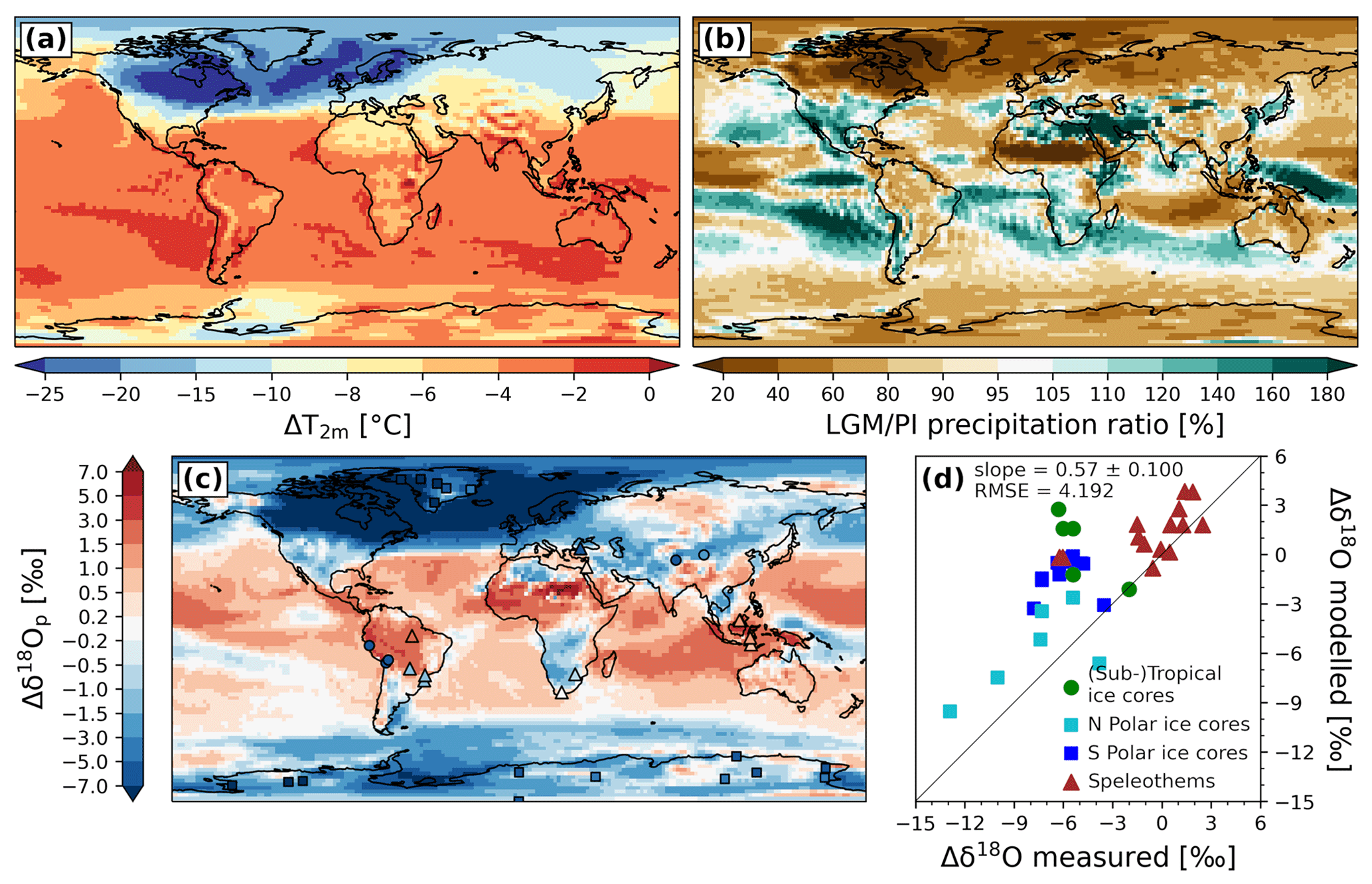
Figure 4(a) LGM–PI 2 m air temperature changes, (b) LGM–PI precipitation ratio, and (c) LGM–PI δ¹⁸O_p anomalies from the LGM_miroc4m_sst_and_sic simulation (background colors). In (c), the squares, dots, and triangles represent δ¹⁸O changes measured in polar ice cores, (sub)tropical ice cores, and speleothems, respectively. Measured δ¹⁸O values in calcite or aragonite from speleothems have been converted into δ¹⁸O of drip water before comparison with modeled δ¹⁸O_p (see Sect. 2.4). (d) Scatter plot showing a comparison of observed δ¹⁸O changes with modeled δ¹⁸O_p anomalies at the nearest grid cell of the archive locations. Northern and southern polar ice core locations are distinguished by cyan and blue, respectively.

The isotope fractionation is mainly controlled by changes in temperature and in the water cycle. Even though all the ECHAM6-wiso simulations show a similar global distribution of 2 m air temperature (T_2 m) and precipitation responses to the various SST and sea ice boundary fields, we find some differences too (Figs. S2 and S3). As expected, the modeled global cooling using SST from GLOMAP is lower, while it is stronger when using SST from Tierney et al. (2020a) (cooling of −4 and −6.3 ^∘C, respectively). Average T_2 m anomalies in the middle range are obtained when using the MIROC 4m SST fields (between −4.4 and −5.3 ^∘C depending on the MIROC 4m data used). The temperatures over sea-ice-covered areas are largely impacted by the sea ice forcings used (i.e., GLOMAP or MIROC 4m). The modeled T_2 m anomalies over the Southern Ocean vary between −10 and −15 ^∘C with an extensive LGM sea ice (GLOMAP), while the cooling is only between −4 and −10 ^∘C when ECHAM6-wiso is forced by a less extensive one (MIROC 4m sea ice). For the Arctic region, a strong cooling is simulated with the very extensive sea ice from MIROC 4m with a weak AMOC phase (a cooling of more than 20 ^∘C), more than with the sea ice from GLOMAP (between −20 and −10 ^∘C). The different SST boundary conditions have a strong influence on the precipitation anomalies, especially at middle to low latitudes including the western Pacific area and the East Asian monsoon region (Fig. S3). All these differences in T_2 m and precipitation responses have profound impacts on modeled δ¹⁸O_p anomalies (Fig. S4) and their agreements with observations (Fig. 4c and d).

Table 3Values of Δδ¹⁸O model–data slope (1 is better), coefficient of determination r², and root mean square error (RMSE) for our ECHAM6-wiso simulations using different SST and sea ice boundary fields. For each column, worst to best model–data agreements are shown with a yellow-to-green color map.

Download Print Version

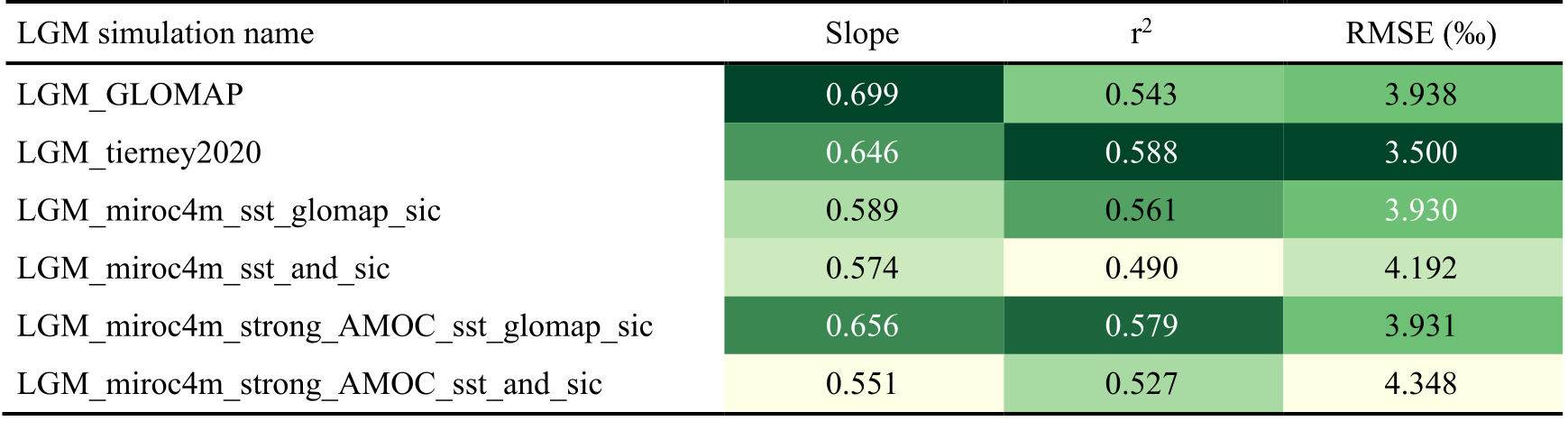
The statistics of Δδ¹⁸O_p model–data agreements are shown for our different ECHAM6-wiso simulations in Table 3. The best model–data agreement in terms of model–data slope (1 is a perfect match) is found when using SST and sea ice from GLOMAP (slope = 0.70) as boundary conditions for ECHAM6-wiso, but a better coefficient of determination (r²) and root mean square error (RMSE) are obtained with LGM SST from Tierney et al. (2020a) (r²= 0.58 and RMSE = 3.5 ‰). We notice worse model–data agreements in δ¹⁸O_p changes when both SST and sea ice changes from MIROC 4m simulations are provided as sea surface boundary conditions (slopes lower than 0.582 and RMSE higher than 4.1 ‰). This is in agreement with Werner et al. (2018), who showed worse model–data agreement when using SST and sea ice boundary conditions from a coupled model instead of reconstructed ones. The substitution of MIROC 4m sea ice changes by GLOMAP ones, which are more extensive in the south and less extensive in the north, improves the Δδ¹⁸O_p model–data agreement for all cases (i.e., weak or strong AMOC phase). For example, the model–data slope when using SST changes from the MIROC 4m simulation during a strong AMOC phase is similar to the one for the simulation with the Tierney et al. (2020a) SST reconstruction (0.66 and 0.65, respectively).

3.2 Impacts of SST boundary conditions on the Δδ¹⁸O model–data agreement at polar ice core stations

The modeled values of Δδ¹⁸O of snow (δ¹⁸O_sn) and ΔT_2 m at polar ice cores stations for different boundary conditions in LGM–PI SST changes are compared to isotopic observations and temperature reconstructions in Fig. 5a. Only simulations using sea ice from GLOMAP are selected here. Except for Renland station in the north and Taylor Dome in the south (both coastal sites), ECHAM6-wiso generally underestimates δ¹⁸O_sn changes. We find generally good agreement with the reconstructed temperature data, except for GRIP station where the cooling is 6–10 ^∘C too weak (dots and crosses in Fig. 5a). The substitution of GLAC-1D reconstruction by the PMIP3 one strongly improves the model–data agreement of δ¹⁸O in Antarctica (Fig. S5), leading to better model–data agreement at the global scale (slope = 0.87, r²= 0.62 and RMSE = 3.2 ‰) compared to the LGM_GLOMAP experiment. This agrees with the findings of Werner et al. (2018), who showed that the isotopic model–data correlation for Antarctic ice core stations is weaker when using GLAC-1D instead of thePMIP3 ice sheet reconstruction (RMSE = 2.1 ‰ and 1.1 ‰ for 11 Antarctic stations, respectively). However, this better Δδ¹⁸O model–data agreement is more likely due to a bias compensation than a more realistic ice sheet because the simulation of Antarctic temperatures by ECHAM6-wiso is degraded at the same time (markers in Fig. S5). Except for the Taylor Dome station, all modeled Δδ¹⁸O_sn values at polar ice core stations are in better agreement with measurements (blue bars in Fig. 5a) when reconstructed SST fields (i.e., GLOMAP or Tierney et al., 2020a) are used (orange and green bars in Fig. 5a, respectively), confirming the results of Werner et al. (2018) about the worse model–data agreement when using sea surface boundary conditions from a coupled model instead of reconstructed ones. The change from one MIROC 4m SST field to another one (i.e., weak or strong AMOC phase) as input for ECHAM6-wiso does not modify the modeled Δδ¹⁸O_sn values much (red and purple bars in Fig. 5a).

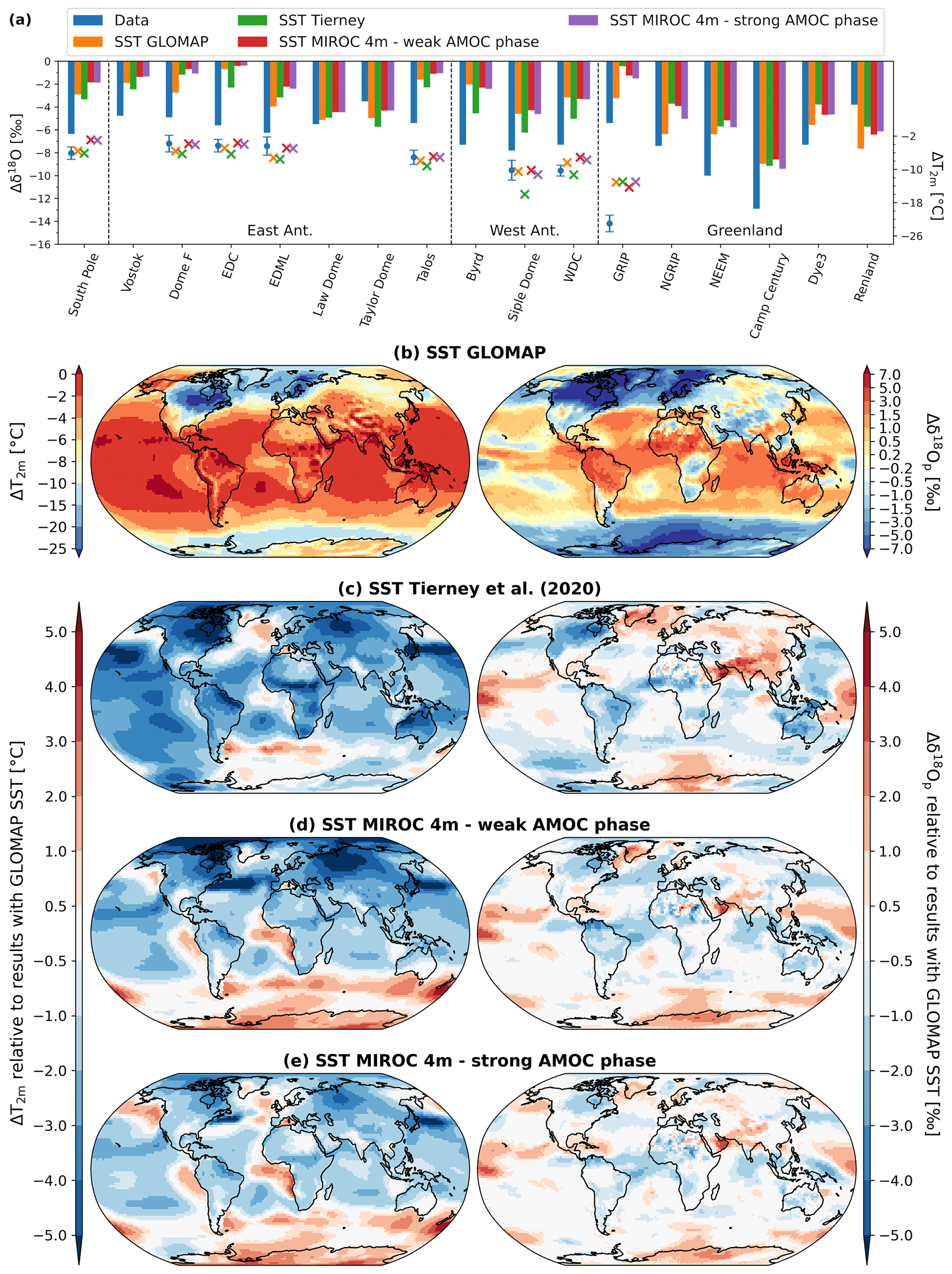
Figure 5(a) Comparison of modeled anomalies in T_2 m (crosses, right vertical axis) and δ¹⁸O_sn (bars, left vertical axis) between LGM and PI with temperature and δ¹⁸O anomalies from polar ice cores (blue dots and bars, respectively). All modeled results are from simulations with the same sea ice boundary conditions from GLOMAP but with different SST forcings: GLOMAP (orange), Tierney et al. (2020a) (green), MIROC 4m with weak LGM AMOC phase (red), and MIROC 4m with strong LGM AMOC phase (purple). (b) Modeled T_2 m and δ¹⁸O_p changes between LGM and PI using GLOMAP SST (left and right maps, respectively). Maps in plots (c) to (e) show the impacts on T_2 m and δ¹⁸O_p anomalies using the other SST boundary conditions. The values are expressed relative to the modeled results from (b).

For a stronger SST cooling in the Southern Ocean (GLOMAP and Tierney et al., 2020a), ECHAM6-wiso simulates higher δ¹⁸O_p changes (right maps of Fig. 5) that are in better agreement with the observations. A stronger cooling in the Atlantic sector of the Southern Ocean (GLOMAP SST compared to the Tierney et al., 2020a, one) has the consequence of enhancing the δ¹⁸O_p depletion in the Atlantic–Indian Ocean sector of Antarctica (right map of Fig. 5c) despite similar temperatures (left map of Fig. 5c). This area includes the ice core stations Dome Fuji and EDML, where better δ¹⁸O and similar temperature model–data agreements are found (orange markers and bars in Fig. 5a). This is also true for other stations further to the east and west, like WDC and EDC (green bars and markers in Fig. 5a). When using an SST field with stronger cooling in the northern North Atlantic Ocean (i.e., GLOMAP), a stronger cooling is simulated there to the south of Greenland. A stronger cooling is simulated in the southern and central parts of inner Greenland too (left maps of Fig. 5) with consequently higher δ¹⁸O changes between LGM and PI in Greenland (right maps of Fig. 5) except in the northern part like at Camp Century station (Fig. 5a). Better agreement is obtained with the Greenland δ¹⁸O observations under this configuration (orange bars in Fig. 5a), without improving the overly weak cooling in the model (colored markers for GRIP station in Fig. 5a).

3.3 Impacts of sea ice change boundary conditions on the Δδ¹⁸O model–data agreement at polar ice core stations

To analyze the effects of sea ice boundary conditions on the modeled δ¹⁸O changes in polar regions between LGM and PI, we compare the results from the simulations using the same SST (here from the MIROC 4m simulation with the weak AMOC phase) but different sea ice area fraction fields: GLOMAP and MIROC 4m (i.e., LGM_miroc4m_sst_ glomap_ sic and LGM_miroc4m_sst_and_sic simulations, respectively). For all Antarctic ice core stations, a stronger depletion in δ¹⁸O_sn between LGM and PI is simulated when the LGM sea ice in the Southern Ocean is more extensive (GLOMAP, orange bars in Fig. 6a). Except for Taylor Dome, better agreement with isotopic observations is then found as is better agreement with temperature reconstructions in West Antarctica. It has a huge impact on modeled T_2 m anomalies over the Southern Ocean (between 2 and 10 ^∘C), and the simulated cooling is higher by 1 to 4 ^∘C in western Antarctica and in coastal regions of the continent (left map of Fig. 6c). As a consequence, higher LGM–PI anomalies in δ¹⁸O of precipitation and snow are simulated: more than 5 ‰ over the Southern Ocean and around 1 ‰–2 ‰ on the continent, especially in the western part (right map of Fig. 6c). More extensive northern sea ice (i.e., MIROC 4m) increases the cooling by 5 to 10 ^∘C in the Arctic Ocean and from 0.5 to 5 ^∘C in Greenland (left map of Fig. 6c), giving higher δ¹⁸O_p anomalies of up to 2 ‰ (right map of Fig. 6c) generally in better agreement with the temperature and δ¹⁸O observations (green bars and markers in Fig. 6a). The opposite is true with the less extensive sea ice distribution from MIROC 4m under a strong AMOC phase, weakening the model–data agreement for Greenland (Fig. S6). A smaller sea ice area fraction in grid cells near coastal areas in MIROC 4m compared to GLOMAP (95 %–98 % against 100 %, respectively. See Sect. 2.2.2), resulting in less important LGM–PI sea ice change, makes the cooling near the Greenland coast slightly lower. This lower sea ice change in MIROC 4m combined with the isotopic content of snow on sea ice taken into account for sublimation processes in sea-ice-covered regions leads to a reduction of the LGM–PI δ¹⁸O_p changes in Baffin Bay (right map of Fig. 6c). This aspect is investigated in detail in Sect. 4.2.

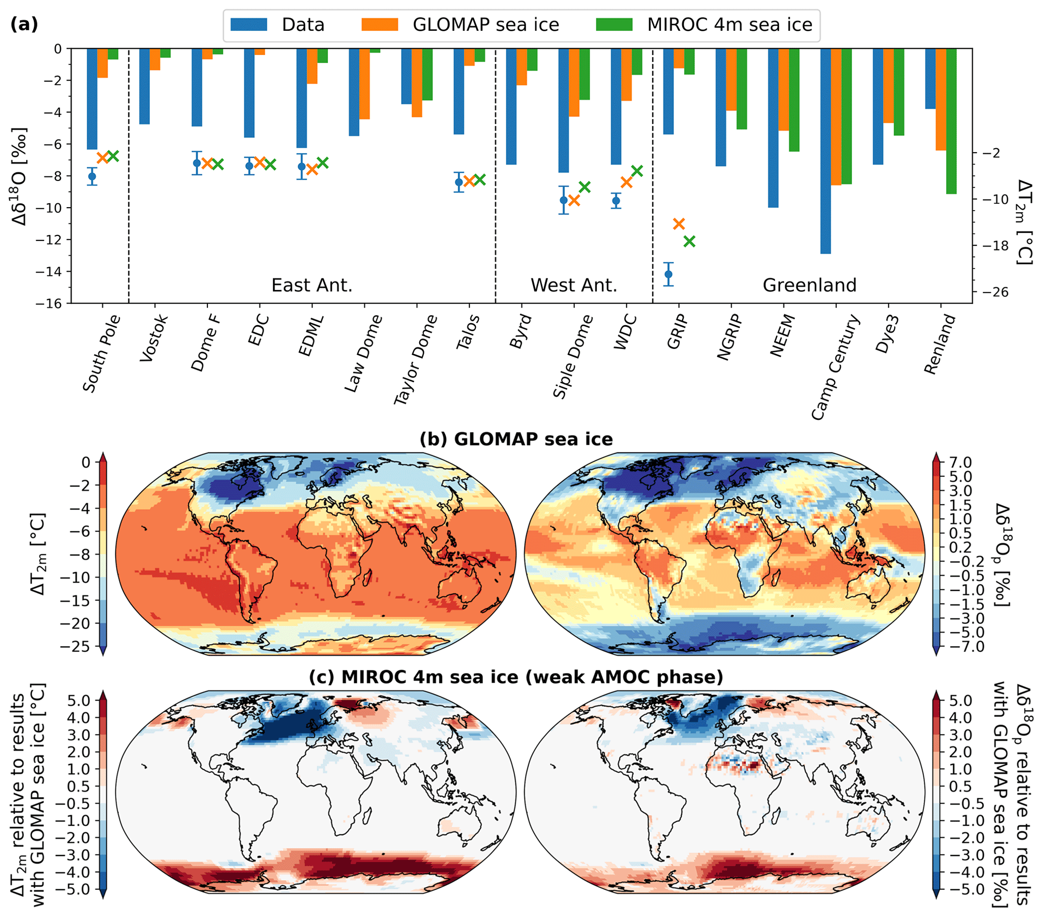
Figure 6(a) Comparison of modeled anomalies in T_2 m (crosses, right vertical axis) and δ¹⁸O_sn (bars, left vertical axis) between LGM and PI with temperature and δ¹⁸O anomalies from polar ice cores (blue dots and bars, respectively). Modeled results are from the simulations using the SST changes of MIROC 4m with weak LGM AMOC but different sea ice boundary conditions (GLOMAP and MIROC 4m with weak LGM AMOC phase in orange and green, respectively). (b) Modeled T_2 m and δ¹⁸O_p changes between LGM and PI using GLOMAP sea ice (left and right maps, respectively). Maps in (c) show the impacts on T_2 m and δ¹⁸O_p anomalies using sea ice from MIROC 4m instead. Values are expressed relative to the modeled results from (b).

3.4 Impacts of LGM AMOC strength on the Δδ¹⁸O model–data agreement at polar ice core stations

Here, we investigate the impacts of AMOC strength on the modeled Δδ¹⁸O in polar regions. For that, sea surface outputs (i.e., both SST and sea ice spatial distribution) from the MIROC 4m simulation with different LGM AMOC strengths are used as boundary conditions for ECHAM6-wiso. We focus first on the North Pole region because the AMOC strength mainly influences the climate of the Northern Hemisphere, as shown in SST and sea ice distributions used in this study (Figs. 1 and 2). A weaker AMOC during the LGM involves less heat transported in the north and thus lower LGM temperatures (i.e., larger cooling relative to PI), as shown in the left map of Fig. 7c. A difference in T_2 m of up to 10 ^∘C in the North Atlantic and Arctic oceans is seen in the LGM_miroc4m_strong_AMOC_sst_glomap_sic and LGM_miroc4m_ strong_AMOC_sst_and_sic simulations. Cooling in Greenland is reduced by 2 to 6 ^∘C when the AMOC is increased, increasing the warm bias in GRIP (markers in Fig. 7a). LGM-to-PI changes in δ¹⁸O in Greenland are mainly controlled by this change in mean temperature with an increase in LGM δ¹⁸O_sn of between 1.2 and 2.5 ‰ at Greenland ice core stations for a stronger LGM AMOC (orange and green bar in Fig. 7a). As ECHAM6-wiso generally underestimates the LGM–PI δ¹⁸O changes at the poles, a weaker AMOC generally improves the model–data agreement (blue and orange bars in Fig. 7a). In the Southern Ocean and Antarctic regions, only small T_2 m changes are simulated by ECHAM6-wiso due to a change in AMOC strength during LGM (left map of Fig. 7c), as shown by the absence of any effect on model–data temperature agreement (markers in Fig. 7a). As a consequence, modeled Δδ¹⁸O_sn values are very similar between the two simulations (orange and green bars in Fig. 7a). These small differences are due to the selection of the strong AMOC phase period in the middle of the peak in the MIROC 4m simulation (see Sect. 2.2.1). The impact of the period selection for the strong AMOC phase (e.g., the start or the end of the interstadial) on surface temperature and δ¹⁸O in Antarctica will be investigated in more detail in a future study. Finally, the SST values alone due to AMOC strength variations change by only less than 1 ‰ of the modeled Δδ¹⁸O_sn (red and purple bars in Fig. 5a). This shows that the LGM-to-PI changes in sea ice distribution, related to the AMOC strength variations, have a large impact on modeled T_2 m anomalies and consequently on the isotopic signals in the North Pole region.

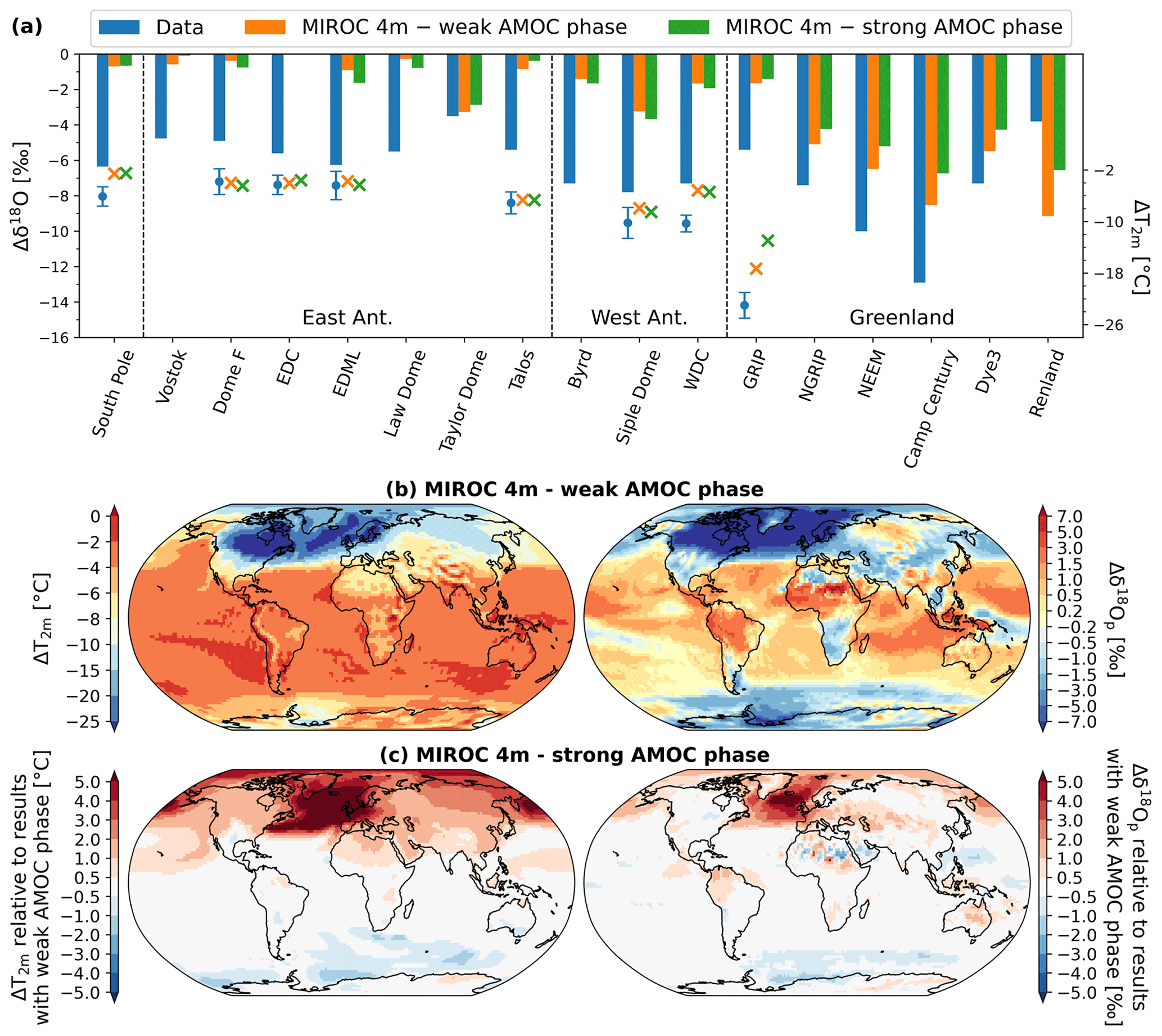
Figure 7(a) Comparison of modeled anomalies in T_2 m (crosses, right vertical axis) and δ¹⁸O_sn (bars, left vertical axis) between LGM and PI with temperature and δ¹⁸O anomalies from polar ice cores (blue dots and bars, respectively). Modeled results are from simulations using the sea surface boundary conditions from the MIROC 4m coupled simulations: LGM_miroc4m_sst_and_sic and LGM_miroc4m_strong_AMOC_sst_and_sic in orange and green, respectively. (b) Modeled T_2 m and δ¹⁸O_p changes between LGM and PI using MIROC 4m (weak AMOC phase) sea surface boundary conditions (left and right maps, respectively). Maps in (c) show the impacts on T_2 m and δ¹⁸O_p anomalies using sea surface boundary conditions from MIROC 4m in a strong LGM AMOC phase. Values are expressed relative to the modeled results from (b).

4.1 Antarctica

Water vapor δ¹⁸O at coastal and western low-elevation sites is controlled by nearby local sources, while the evaporative moisture source of high-elevation East Antarctic ice cores is typically further north at around 40–45^∘ S (Sodemann and Stohl, 2009). So, the values of the δ¹⁸O_p–T_2 m slope in Antarctica are expected to be influenced by sea surface boundary conditions in different ways depending on the ice core site location and elevation.

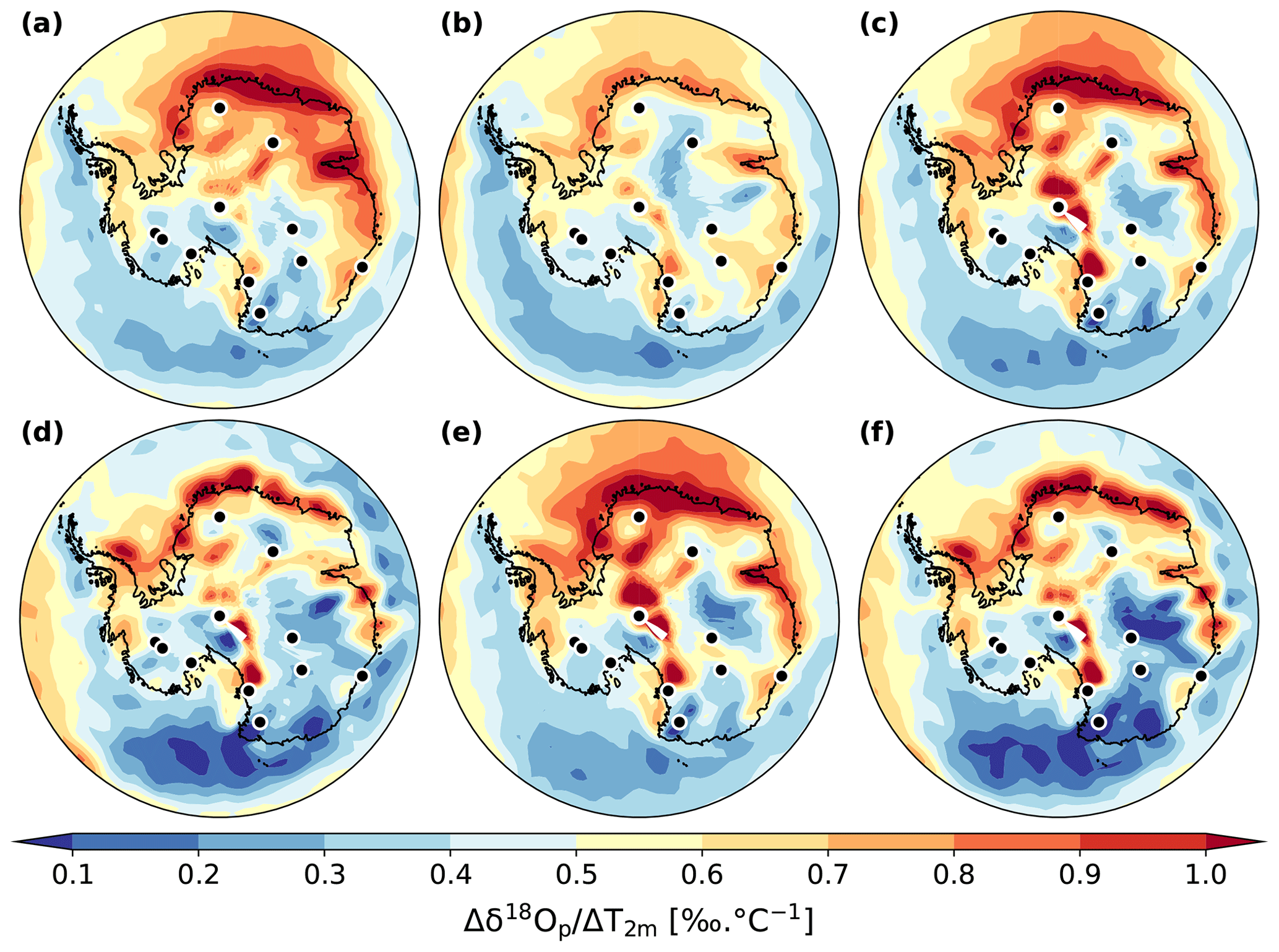
Figure 8Spatial distribution of the δ¹⁸O_p–T_2 m temporal slope in Antarctica for LGM–PI changes according to our different ECHAM6-wiso simulations: (a) LGM_GLOMAP, (b) LGM_tierney2020, (c) LGM_miroc4m_sst_glomap_sic, (d) LGM_miroc4m_sst_and_sic, (e) LGM_miroc4m_strong_ AMOC_ sst_glomap_sic, and (f) LGM_miroc4m_strong_ AMOC_ sst_and_sic. The dots indicate the location of the ice core stations.

Greater SST cooling in the Southern Ocean influences both the LGM T_2 m and δ¹⁸O_p in the same direction (i.e., toward lower values) but with different magnitudes. Stronger cooling in the eastern part of the ocean (Tierney et al., 2020a, LGM SST is colder than the GLOMAP one) increases the temporal slopes at EDC and Talos Dome by 0.23 ‰ ^∘C⁻¹ and 0.07 ‰ ^∘C⁻¹, respectively. A higher cooling in the Atlantic sector of the Southern Ocean (GLOMAP SST in Fig. 8a) makes the Antarctic temporal slope values higher between 0 and 90^∘ E longitude compared to the other simulations (meaning that δ¹⁸O_p is more impacted than temperature). It especially impacts the Dome Fuji and EDML ice core sites, where values of temporal δ¹⁸O_p–T_2 m slopes reach 0.66 ‰ ^∘C⁻¹ and 0.69 ‰ ^∘C⁻¹, representing an increase of at least 25 % compared to simulations using SST with less cooling. This can be explained by a change in moisture transport. With a stronger SST cooling in the Southern Ocean (GLOMAP against MIROC 4m), the westerlies around Antarctica are enhanced and the atmosphere is wetter in the midlatitudes, while a drier belt appears around the continent (Fig. 9b). More water vapor from the Atlantic sector at 30–40^∘ S, where the cooling is less strong (compared to MIROC 4m SST) and the water vapor more depleted in δ¹⁸O (Fig. S4a) because of enhanced evaporation, is transported to eastern Antarctica. As a consequence, the larger cooling in GLOMAP Southern Ocean SST increases the temporal slope at Dome Fuji and EDML stations. A larger SST cooling near the Amundsen Sea (i.e., Tierney et al., 2020a, SST compared to GLOMAP, Fig. 5c) impacts the temperature from this region to western Antarctic sites (2 to 4 ^∘C, left map of Fig. 5c). On the other hand, the δ¹⁸O of water vapor and precipitation in the Amundsen Sea area is not so impacted by imposed stronger SST cooling (by 2 ‰ at maximum, right map of Fig. 5c). The decrease in the transport of this not-so-depleted water vapor to western Antarctic sites (Fig. S7) increases the temporal slopes by ∼ 0.1 % ^∘C⁻¹ at WDC and Byrd stations (orange marker in Fig. 12). At the same time, this water vapor influences the δ¹⁸O_p of nearby coastal regions like the Antarctic peninsula, decreasing their temporal slopes (Fig. 8b and orange marker in Fig. S9).

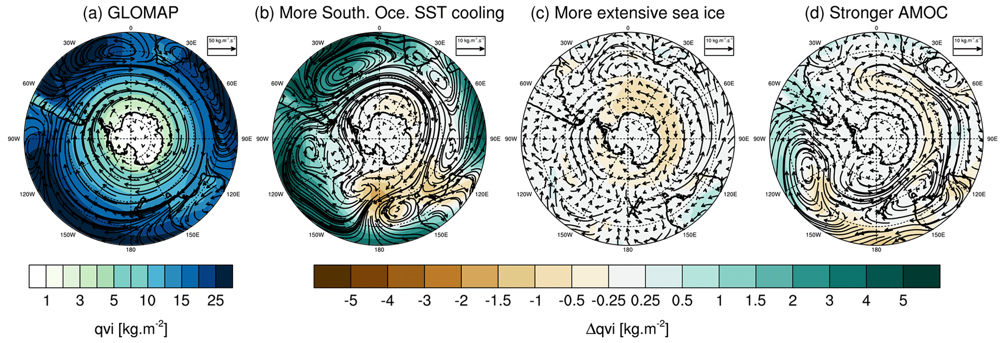
Figure 9(a) Vertically integrated water vapor transport (arrows) and total column water vapor (qvi, colored background) in the LGM_GLOMAP simulation over the Antarctic region. Anomalies in transport and concentration of moisture are shown for (b) a stronger SST cooling in the Southern Ocean (LGM_GLOMAP − LGM_miroc4m_sst_glomap_sic), (c) more extensive sea ice (LGM_miroc4m_sst_glomap_sic − LGM_miroc4m_sst_ and_ sic), and (d) a stronger LGM AMOC (LGM_miroc4m_strong_AMOC_sst_and_sic − LGM_miroc4m_sst_and_sic).

LGM-to-PI changes in sea ice area fractions have a strong impact on the slopes in coastal regions, as shown by the comparison between plots (c)–(d) and (e)–(f) in Fig. 8. Law Dome ice core is representative of this impact in coastal areas, with a slope of 0.35 ‰ ^∘C⁻¹ and 0.64 ‰ ^∘C⁻¹ depending on whether less extensive sea ice (LGM_miroc4m_sst_and_sic, Fig. 8d) or more extensive sea ice (LGM_miroc4m_sst_glomap_sic, Fig. 8c) is used, respectively. More extensive sea ice in the Atlantic and Indian sectors of the Southern Ocean changes the transport of vapor only slightly (Fig. 9c). On the other hand, the presence of more sea-ice-covered area close to the continent increases the amount of local water vapor depleted in δ¹⁸O (compared to the δ¹⁸O of open seawater) that influences the isotopic composition of snow in coastal sites, increasing their temporal slopes. The more extensive sea ice in the Indian sector of the Southern Ocean increases the slope in a geographical band from Law Dome to Vostok and EDC stations (Fig. 8c and d). This can be explained by a decrease in transport of enriched water vapor from the Indian Ocean and marine region south of Australia, especially in austral winter (Fig. S9). On average, the modeled temporal δ¹⁸O_p–T_2 m slopes of East Antarctic ice core stations are increased by more than 25 % when more extensive sea ice is used (Fig. 12, dark and light purple markers against the red and grey ones, respectively). This conclusion remains the same when using the average slope across the entire East Antarctic area but with an enhanced difference because the entire coastal area is under consideration (Fig. S9). No clear influence of sea ice extent on temporal slopes at West Antarctica ice core stations is found (Fig. 12). On the other hand, effects on the Antarctic peninsula, Ronne Ice Shelf, and the coast of the Amundsen Sea (Fig. 8), influencing the average slope values in the entire western part of the continent (Fig. S9), are simulated. These are due to changes in the nature of the water source nearby (i.e., open water or sea ice) depending on whether the sea ice used is less extensive or not.

4.2 Greenland

Using an SST field with more LGM cooling off the coast of Greenland and in the northern North Atlantic Ocean (GLOMAP) as forcing for ECHAM6-wiso, we model higher δ¹⁸O_p–T_2 m temporal slope values at all Greenland ice core stations (Fig. 10a) compared to all other simulations. The average of the temporal slope values at ice core stations is 0.50 ‰ ^∘C⁻¹ with GLOMAP sea surface boundary forcing (blue marker in Fig. 12) and less than 0.42 ‰ ^∘C⁻¹ in the other ECHAM6-wiso simulations. This difference is enhanced by considering the entire Greenland area (blue marker in Fig. S9). For Greenland, most of the moisture comes from northern North Atlantic Ocean at latitudes 30–40^∘ N (Drumond et al., 2016), south of the ice sheet (Fig. 11a). A stronger SST cooling in the Arctic–North Atlantic enhances the transport of isotopically depleted water vapor from North America (Fig. 11b) and strengthens the water vapor transport belt around Iceland. Also, ECHAM6-wiso simulates a slight decrease in local water vapor content in the Greenland Sea (with lower LGM δ¹⁸O because the cooling is stronger there) and its transport to land. It increases the isotope–temperature temporal slope from the sea to the inland area, passing through the eastern Greenland coast where Renland station is located (Fig. 10b and c compared to a).

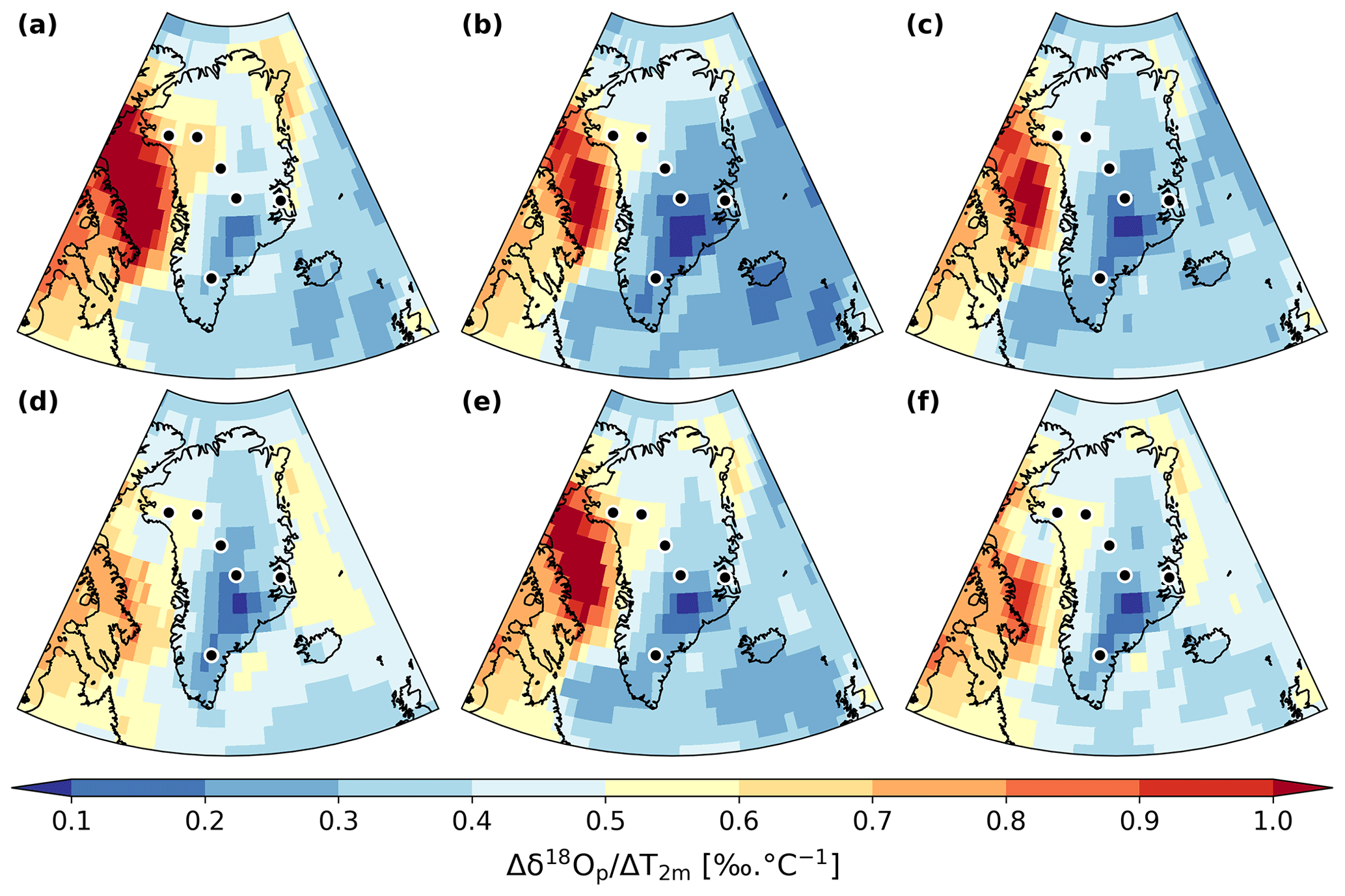
Figure 10Same as Fig. 8 but for the Greenland region.

More extensive sea ice (i.e., MIROC 4m compared to GLOMAP) makes the Arctic Ocean area drier, especially at 50^∘ N, and it slightly slows down the transport of water vapor from the North Atlantic to Greenland area (Fig. 11c). On the other hand, all this area is covered by sea ice in the “more extensive sea ice” simulation (i.e., MIROC 4m sea ice). It decreases the δ¹⁸O of water vapor above this surface, increasing the isotope–temperature temporal slope on the eastern Greenland coast and in the Greenland Sea (Fig. 10d and f compared to c and e, respectively). In the latter, more extensive sea ice, especially in summer, decreases the LGM δ¹⁸O too, while the effect on temperature is small, again increasing the local temporal slope. It has a slight effect on modeled temporal slopes (∼ 0.1 ‰ ^∘C⁻¹) over the eastern coastal regions of Greenland, including Renland station. In ECHAM6-wiso, the isotopic composition of sea ice surfaces also reflects the isotopic composition of snow deposited on this surface. Then the formation of new sea ice from PI to LGM acts as a positive feedback effect in the decrease in surrounding δ¹⁸O_p, leading to steeper modeled δ¹⁸O_p–T_2 m temporal slopes (see Sect. S1 and Fig. S10). Finally, ECHAM6-wiso forced with MIROC 4m sea ice, whose fractional areas are artificially lower (i.e., not 100 % sea-ice-covered) in coastal grid cells, simulates lower δ¹⁸O_p–T_2 m temporal slope values over Baffin Bay (between 0.3 ‰ ^∘C⁻¹ and 0.9 ‰ ^∘C⁻¹, Fig. 9d and f) compared to when the model is forced with GLOMAP sea ice (between 0.6 and 1.25 ‰ ^∘C⁻¹, Fig. 10c and e). If the MIROC 4m sea ice is corrected by setting the sea ice fraction as 100 ‰ as in GLOMAP (see Sect. S1 and Fig. S11), we obtain temporal slope values similar to those in the simulations forced by GLOMAP sea ice (Fig. S12).

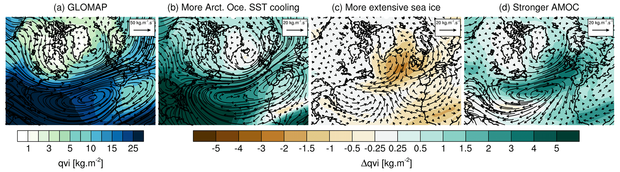
Figure 11(a) Vertically integrated water vapor transport (arrows) and total column water vapor (qvi, colored background) in the LGM_GLOMAP simulation over the Arctic region. Anomalies in transport and concentration of moisture are shown for (b) a stronger SST cooling in Arctic Ocean (LGM_GLOMAP − LGM_tierney2020), (c) more extensive sea ice (LGM_miroc4m_sst_and_sic − LGM_miroc4m_sst_glomap_sic), and (d) a stronger LGM AMOC (LGM_miroc4m_strong_AMOC_ sst_and_sic − LGM_miroc4m_sst_and_sic).

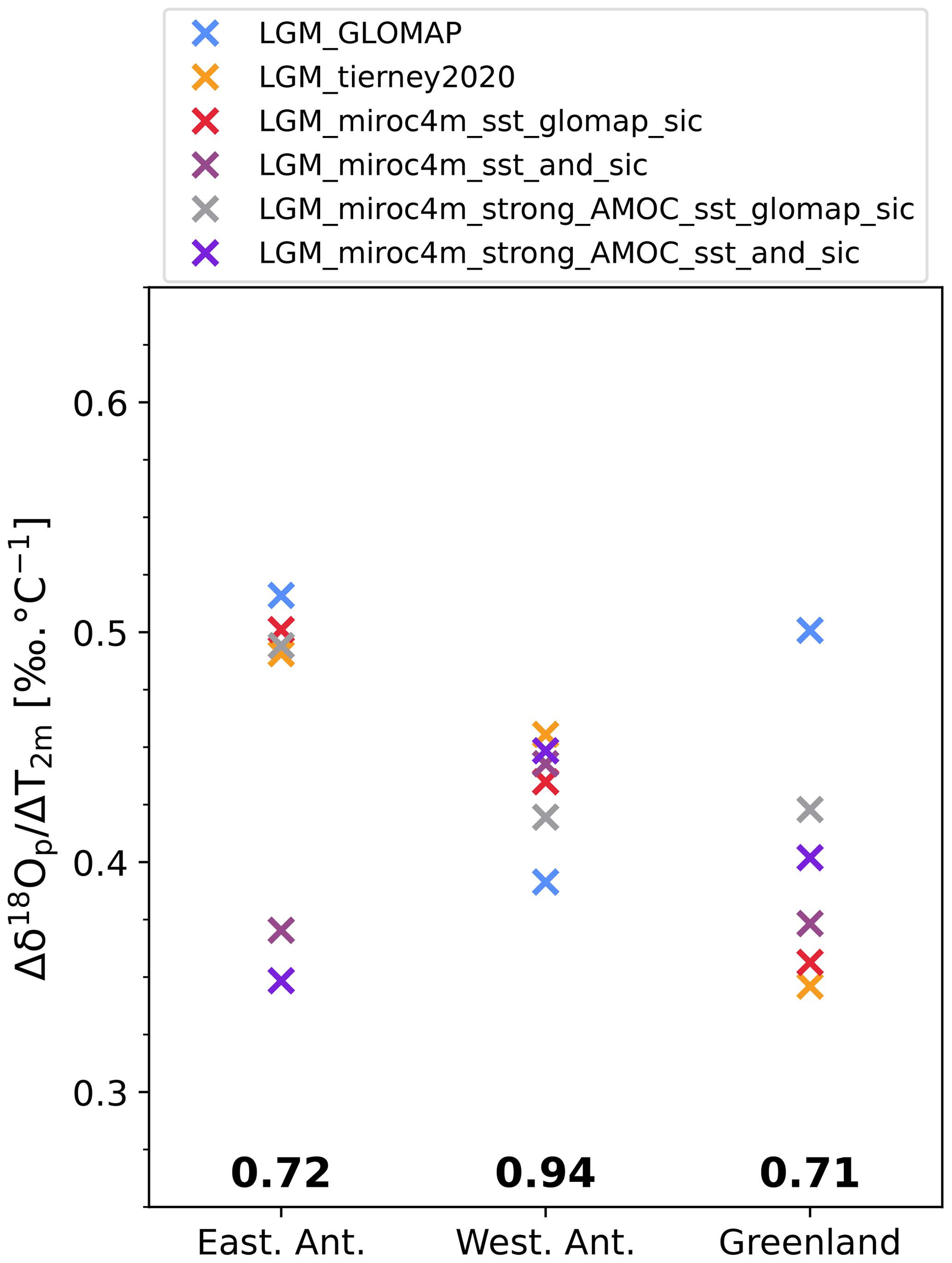
Figure 12Average modeled values of the δ¹⁸O_p–T_2 m temporal slope for East Antarctic, West Antarctic, and Greenland ice core stations according to our different simulations. Numbers in bold are the values of the corresponding modeled mean PI spatial slopes.

Download

A stronger AMOC increases the amount of water vapor and enhances its transport from the North Atlantic to European coastal areas because of the less extensive sea ice (Fig. 11d). More water vapor with higher δ¹⁸O is present southeast of Greenland because sea ice is replaced by open water. However, there is only a slight increase in the transport of this water vapor toward north in the Greenland interior (Fig. 11d), while the cooling inland is largely reduced (Fig. 7c). So, isotope–temperature temporal slopes are slightly increased over the interior of Greenland for stronger AMOC (dark and light purple markers in Figs. 12 and S9). On the other hand, temporal slopes are decreased over the Greenland Sea (Fig. 10f) because of the presence of open water instead of sea ice, enhancing the LGM δ¹⁸O_p locally. Note that stronger AMOC worsens the model–data agreement for both ΔT_2 m and Δδ¹⁸O (Fig. 7a).

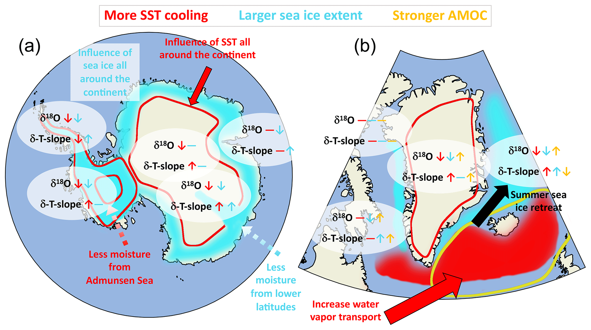
Figure 13Summary figure illustrating the influence of higher sea surface cooling, larger sea ice extent, and stronger LGM AMOC (in red, cyan, and yellow, respectively) on the modeled LGM δ¹⁸O and temporal δ¹⁸O_p–T_2 m slopes in the Antarctic and Greenland regions (a and b, respectively). The up and down arrows indicate higher and lower values, respectively. The horizontal lines indicate no significant change.