the Creative Commons Attribution 4.0 License.
the Creative Commons Attribution 4.0 License.
 | 16 Nov 2020
Revisiting the trend in the occurrences of the “warm Arctic–cold Eurasian continent” temperature pattern
Lejiang Yu
Shiyuan Zhong
Cuijuan Sui
Bo Sun
The recent increasing trend of “warm Arctic, cold continents” has attracted much attention, but it remains debatable as to what forces are behind this phenomenon. Here, we revisited surface temperature variability over the Arctic and the Eurasian continent by applying the self-organizing-map (SOM) technique to gridded daily surface temperature data. Nearly 40 % of the surface temperature trends are explained by the nine SOM patterns that depict the switch to the current warm Arctic–cold Eurasia pattern at the beginning of this century from the reversed pattern that dominated the 1980s and 1990s. Further, no cause–effect relationship is found between the Arctic sea ice loss and the cold spells in the high-latitude to midlatitude Eurasian continent suggested by earlier studies. Instead, the increasing trend in warm Arctic–cold Eurasia pattern appears to be related to the anomalous atmospheric circulations associated with two Rossby wave trains triggered by rising sea surface temperature (SST) over the central North Pacific and the North Atlantic oceans. On interdecadal timescale, the recent increase in the occurrences of the warm Arctic–cold Eurasia pattern is a fragment of the interdecadal variability of SST over the Atlantic Ocean as represented by the Atlantic Multidecadal Oscillation (AMO) and over the central Pacific Ocean.


In recent decades, winter season temperature in the Arctic has been rising at a rate faster than the warming experienced in any other regions of the world (Stroeve et al., 2007; Screen and Simmonds, 2010; Stroeve, 2012). In contrast, there has been an increasing trend in colder-than-normal winters over the northern midlatitude continents (Mori et al., 2014; Cohen et al., 2014, 2018). This pattern of opposite winter temperature trend between the Arctic and high-latitude to midlatitude continents, referred to as the “warm Arctic–cold continents” pattern (Overland et al., 2011; Cohen et al., 2014; Walsh, 2014), has received considerable interest in the scientific community especially with regard to dynamical and physical mechanisms for the development of the phenomenon (Mori et al., 2014; Vihma, 2014; Barnes and Screen, 2015; Kug et al., 2015; Overland et al., 2015; Chen et al., 2018).
Using observational analyses or coupled ocean–atmosphere modeling, a number of studies have attributed the recent warm Arctic–cold continents pattern to the Arctic sea ice loss in boreal winter (Inoue et al., 2012; Tang et al., 2013; Mori et al., 2014; Kug et al., 2015; Cohen et al., 2018; Mori et al., 2019). Sea ice variability in different parts of the Arctic Ocean has been linked to climate variability in different parts of the world. Specifically, sea ice loss in the Barents and Kara seas has been linked to cold winters over East Asia (Kim et al., 2014; Mori et al., 2014; Kug et al., 2015; Overland et al., 2015) and in central Eurasia (Mori et al., 2014), while a similar connection has been found between cold winters in North America and sea ice retreat in the East Siberian and Chukchi seas (Kug et al., 2015). A more recent study (Matsumura and Kosaka, 2019) attributed the warm Arctic–cold continents pattern to the combined effect of Arctic sea ice loss and the atmospheric teleconnection induced by tropical Atlantic sea surface temperature (SST) anomalies.
Other studies, however, found no cause-and-effect relationship between Arctic sea ice loss and midlatitude climate anomalies (Blackport et al., 2019; Fyfe, 2019). Numerical modeling studies using coupled ocean and atmospheric models simulated no cold midlatitude winters when the models were forced with reduced Arctic sea ice cover (McCusker et al., 2016; Sun et al., 2016; Blackport et al., 2019; Fyfe, 2019). Instead, these studies pointed to internal atmospheric variability as the likely cause for cold winters in midlatitudes. Some studies have also suggested that on the interannual timescale midlatitude atmospheric circulation anomalies triggered by the Pacific and Atlantic SST oscillations may explain both the Arctic sea ice loss and the cooling of the high latitudes to midlatitudes (Lee et al., 2011; Luo et al., 2016; Peings et al., 2019; Matsumura and Kosaka, 2019; Clark and Lee, 2019). The sea surface temperature anomalies over the Gulf Stream have also been linked to the Barents Sea ice loss and Eurasian cooling (Sato et al., 2014).
Despite the recent attention given to the warm Arctic–cold continents pattern, the roles various dynamical and physical processes play in the formation of this phenomenon remain debatable. In this study, we revisit surface temperature variability over the Arctic and the Eurasian continent (40–90∘ N, 20–130∘ E), where the warm Arctic–cold continents pattern is a prominent feature (Cohen et al., 2014; Mori et al., 2014), by applying the self-organizing-map (SOM) technique to daily surface temperature over the recent four decades. We will show that while the warm Arctic–cold Eurasian continent pattern has dominated the recent two decades, its opposite pattern, cold Arctic–warm Eurasian continent, appeared frequently in the 1980s and 1990s. Using century-long data, we will further show that the warm Arctic–cold Eurasian continent pattern is an intrinsic climate mode and the recent increasing trend in its occurrence is a reflection of an interdecadal variability of the pattern. Using linear regression, we explain the reason for the recent increasing occurrences of the warm Arctic–cold continents pattern. We also assess the role of the SST anomalies over the North Pacific and Atlantic oceans in the variability of the warm Arctic–cold Eurasia pattern on the interdecadal timescale.
2.1 Datasets
Daily surface air temperature and other climate variables used in the current analyses, including 500 hPa geopotential height, 800 hPa wind, and mean sea level pressure, all come from the European Centre for Medium-Range Weather Forecasts (ECMWF) interim reanalysis (ERA-Interim; Dee et al., 2011) with a horizontal resolution of approximately 79 km (T255) and 60 vertical levels in the atmosphere. Compared to the earlier versions of ERA (e.g., ERA-40; Uppala et al., 2005) and other global reanalysis products (e.g., the NCEP reanalysis; Kalnay et al., 1996), ERA-Interim has been found to be more accurate in portraying the Arctic warming trend (Dee et al., 2011; Screen and Simmonds, 2011) despite its known warm and moist bias in the surface layer (Jakobson et al., 2012). Daily sea ice data are obtained from the US National Snow and Ice Data Center (NSIDC; ftp://sidads.colorado.edu/DATASETS/nsidc0051_gsfc_nasateam_seaice/final-gsfc/north/daily, last access: 31 August 2020). Gridded monthly SST data used in the current analysis are obtained from the US National Oceanic and Atmospheric Administration (NOAA) data archives (ftp://ftp.cdc.noaa.gov/Datasets/noaa.oisst.v2.highres/, last access: 3 July 2020) (Reynolds et al. 2007). In our analyses, we retain the trends in the data over the 1979–2019 period.
The results obtained from the data within the recent four decades are put into the context of the variability over longer timescales using data from the 20th Century Reanalysis project version 2C (20CR), which spans more than a century (from 1851 to 2015) (Compo et al., 2011). The 20CR reanalysis data, which have a horizontal resolution of 2∘ latitude by 2∘ longitude and temporal resolution of 6 h, were produced by a model driven at the lower boundary by observed monthly SST and sea ice conditions and with data assimilation of surface pressure observations. Several indices used to describe known modes of climate variability, including the Arctic Oscillation (AO), Northern Atlantic Oscillation (NAO), Atlantic Multidecadal Oscillation (AMO) (Enfield et al., 2001), and Pacific Decadal Oscillation (PDO) (Mantua et al., 1997), are obtained from NOAA's Climate Prediction Center (CPC) (https://www.esrl.noaa.gov/psd/data/climateindices/list/, last access: 21 March 2020).
Table 1Spatial correlation (Corr) between the daily winter (December, January, and February; DJF) surface air temperature and the corresponding SOM pattern for each day from 1979 to 2018.
2.2 Methods
From the perspective of nonlinear dynamic, a region's climate has its intrinsic modes of variability, but the frequency of occurrence of these internal modes can be modulated by remote forces external to the region (Palmer, 1999; Hoskins and Woollings, 2015; Shepherd, 2016). In this study, we will first obtain the main modes of variability of wintertime surface temperature in a region (40–90∘ N, 20–130∘ E) by applying the SOM method (Kohonen, 2001) to daily surface temperature data for the 40 winters (December, January, February) from December 1979 to February 2019. The use of daily data over four decades allows for capturing the variability across two timescales (synoptic and decadal). SOM is a clustering method based on a neural network that can transform multi-dimensional data into a two-dimensional array without supervised learning. The array includes a series of nodes arranged by a Sammon map (Sammon, 1969). Each node in the array has a vector that can represent a spatial pattern of the input data. The distance of any two nodes in the Sammon map represents the level of similarity between the spatial patterns of the two nodes. Because SOM has fewer limitations than most other commonly used clustering methods (e.g., orthogonality required by the empirical orthogonal function or EOF method), the SOM method can better describe the main variability patterns of the input data (Reusch et al., 2005).
The SOM method has been used in atmospheric research at midlatitudes and high latitudes of the Northern Hemisphere (Skific et al., 2009; Johnson and Feldstein, 2010; Horton et al., 2015; Loikith and Broccoli, 2015; Vihma et al., 2019). For example, Johnson and Feldstein (2010) used SOM to identify spatial patterns of daily wintertime North Pacific sea level pressure and relate the variability of the occurrences of those patterns to some large-scale circulation indices. Loikith and Broccoli (2015) compared observed and model-simulated circulation patterns across the North American domain using an approaching involving SOM. The SOM method was also used to detect circulation pattern trends in a subset of North America during two different periods (Horton et al., 2015).
In this study, the SOM method is applied to ERA-Interim wintertime daily temperature anomalies from December 1979 to February 2019. The anomalies are calculated by subtracting 40-year-averaged daily temperature from the original daily temperature at each grid point. Prior to SOM analysis, it is necessary to determine how many SOM nodes are needed to best capture the variability in the data. According to previous studies (Lee and Feldstein, 2013; Gibson et al., 2017; Schudeboom et al., 2018), the rule for determining the number of SOM nodes is that the number should be sufficiently large to capture the variability of the data analyzed but not too large to introduce unimportant details. Table 1 shows the averaged spatial correlation between all daily surface air temperature anomalies and their matching nodes. The spatial correlation coefficients increase from 0.26 for a 3×1 grid to 0.51 for a 4×4 grid, but the gain from a 3×3 grid to a 4×4 grid is relatively small. Hence, a 3×3 grid seems to meet the abovementioned rule and will be utilized in this study.
The contribution of each SOM node to the trend in wintertime surface temperature anomalies is calculated by the product of each node pattern and its frequency trend normalized by the total number (90) of wintertime days (Lee and Feldstein, 2013). The sum of the contributions from all nodes denotes the SOM-explained trends. Residual trends are equal to the subtraction of SOM-explained trends from the total trends. The anomalous atmospheric circulation pattern corresponding to each of the SOM pattern is obtained by composite analysis that computes a composite mean of an atmospheric circulation field (e.g., 500 hPa height) over all occurrences of that SOM node. Regression analysis is also performed where atmospheric circulation variables are regressed onto the time series of the occurrence of a SOM node to further elucidate the relationship between the variability of atmospheric circulations and surface temperatures. The statistical significance of composite and regression analyses in this study is tested by using the Student's t test.

Figure 1Spatial patterns of SOM nodes for daily wintertime (DJF) surface air temperature anomalies (∘C) from ERA-Interim reanalysis over the 1979–2019 period. The number in brackets denotes the frequency of the occurrence for each node.
3.1 Surface temperature variability
The majority of the nine SOM nodes depict a dipole pattern characterized by opposite changes in surface temperatures between the Arctic Ocean and the Eurasian continent, although the sign switch does not always occur at the continent–ocean boundary (Fig. 1). The differences in the position of the boundary between the warm and cold anomalies reflects the transition between the cold Arctic–warm Eurasia pattern (denoted, in descending order of the occurrence frequency, by nodes 3, 9, and 6) and the warm Arctic–cold Eurasia pattern (depicted, in descending order of the occurrence frequency, by nodes 1, 7, and 4). The spatial patterns represented by the first group of nodes are almost mirror images of the patterns denoted by the corresponding nodes in the second group. For example, the second node in group 1 (node 9, 15.4 %) and the first node in group 2 (node 1, 17.1 %) show a mirror image pattern with cold (warm) anomalies in the Arctic Ocean extending into northern Eurasia and warm (cold) anomalies in the rest of the Eurasian continent in the study domain. In both cases, the region of maximum magnitude anomalies is centered near Svalbard, Norway. The second pair, denoted by node 3 (17.2 %) and 7 (13.7 %), has the boundary of separation moved northward from the northern Eurasian continent toward the shore of the Arctic Ocean. While the maximum anomaly in the Arctic Ocean remains close to Svalbard, maximum values over the continent are found in central Russia. Nodes 4–6 display a noticeable transition from node 1 to node 7 and from node 3 to node 9, respectively. Although nodes 2 and 8 show an approximate monopole spatial pattern, they also represent a transition between nodes 1 and 3, and between nodes 7 and 9, respectively. The above SOM analysis does not consider the trend in surface air temperature. The result is similar when the trend is removed (not shown).
The temporal variability on this timescale is typically related to synoptic processes, and hence the questions are what synoptic patterns are responsible for the occurrence of the spatial patterns depicted by each of the nine SOM nodes and how these patterns are related to those of the Arctic sea ice anomalies. These questions can be answered by using the composite method. Specifically, for each SOM node, composite maps are made, respectively, for the anomalous 500 hPa geopotential height, mean sea level pressure, 850 hPa wind, downward longwave radiation, surface turbulent heat flux, and sea ice concentration over all the days when the spatial variability of the surface temperature anomalies is best matched by the spatial pattern of that node.
Figure 2Corresponding 500 hPa geopotential height anomalies (gpm) from ERA-Interim reanalysis over the 1979–2019 period for each node in Fig. 1. Dotted regions indicate the above-95 % confidence level. The subdomain in 1 shows the study region.
Figure 3Corresponding anomalous 850 hPa wind field (m s−1) from ERA-Interim reanalysis over the 1979–2019 period for each node in Fig. 1. Shaded regions indicate the above-95 % confidence level.
3.2 Large-scale circulation patterns
For all SOM nodes, the spatial pattern of the composited 500 hPa geopotential height anomalies (Fig. 2) is similar to that of mean sea level pressure anomalies (not shown), indicating an approximately barotropic structure. For nodes 1, 4, and 7, the 500 hPa height anomalies show a dipole structure of positive values over Siberia and negative values to its south over the Eurasian continent. Anomalous southwesterly winds on the western side of the anticyclone over Siberia transport warm and moist air from northern Europe and the North Atlantic Ocean into the Atlantic sector of the Arctic Ocean (Fig. 3), providing a plausible explanation of the warm surface temperature anomalies in the region (Fig. 1). On the eastern side of the anticyclone, anomalous northwesterly winds bring cold and dry air from the Arctic Ocean into the Eurasian continent, which is consistent with the negative surface temperature anomalies there. The opposite occurs for nodes 3, 6, and 9. A similar explanation involving anomalous pressure and wind fields can be applied to other nodes. The dipole structure that dominates the anomalous 500 hPa height fields over the North Atlantic Ocean for most nodes resembles the spatial pattern of the NAO (Fig. 2). In addition, the patterns for several nodes, such as nodes 4 and 7, have some resemblance to the spatial pattern of the AO over larger geographical region. The possible connection to NAO and AO is further investigated by averaging the daily index values of NAO or AO over all occurrence days for each node. The results (Table 2) show that nodes 1, 2, and 3 (5, 8, and 9) correspond to a significant positive (negative) phase of the NAO index characterized by negative (positive) height anomalies over Iceland and positive (negative) values over the central North Atlantic Ocean. Association is also found between nodes 1, 2, 3, and 6 (5, 7, 8, and 9) and the positive (negative) phases of the AO index.
Table 2Averaged anomalous NAO and AO indices for all occurrences of each SOM node. Asterisks indicate the above-95 % confidence level.
3.3 Downward radiative fluxes
Besides the anomalous circulation patterns, anomalous surface radiative fluxes may also play a role in shaping the spatial pattern of surface temperature variability. In fact, the spatial pattern of the mean anomalous daily downward longwave radiation for an individual node (Fig. 4) is in good agreement with the spatial pattern of the surface temperature anomalies of that node. In other words, increased downward longwave radiation is associated with positive surface temperature anomalies, and vice versa. As expected from previous studies (e.g., Sedlar et al. 2011), there is a significant positive correlation between downward longwave radiative fluxes and the anomalous total column water vapor and mid-level cloud cover (not shown). The correlation to low- and high-level cloud cover is, however, not significant (not shown). Most of the water vapor in both the Arctic and Eurasia is derived from the North Atlantic Ocean, but the water vapor is transported into the Arctic by southwesterly flows and into Eurasia by northwesterly winds. The anomalous shortwave radiation corresponding to each node (not shown) is an order of magnitude smaller than that of the longwave radiation anomalies and has a spatial pattern opposite to that of the mid-level cloud cover and the longwave radiation anomalies.
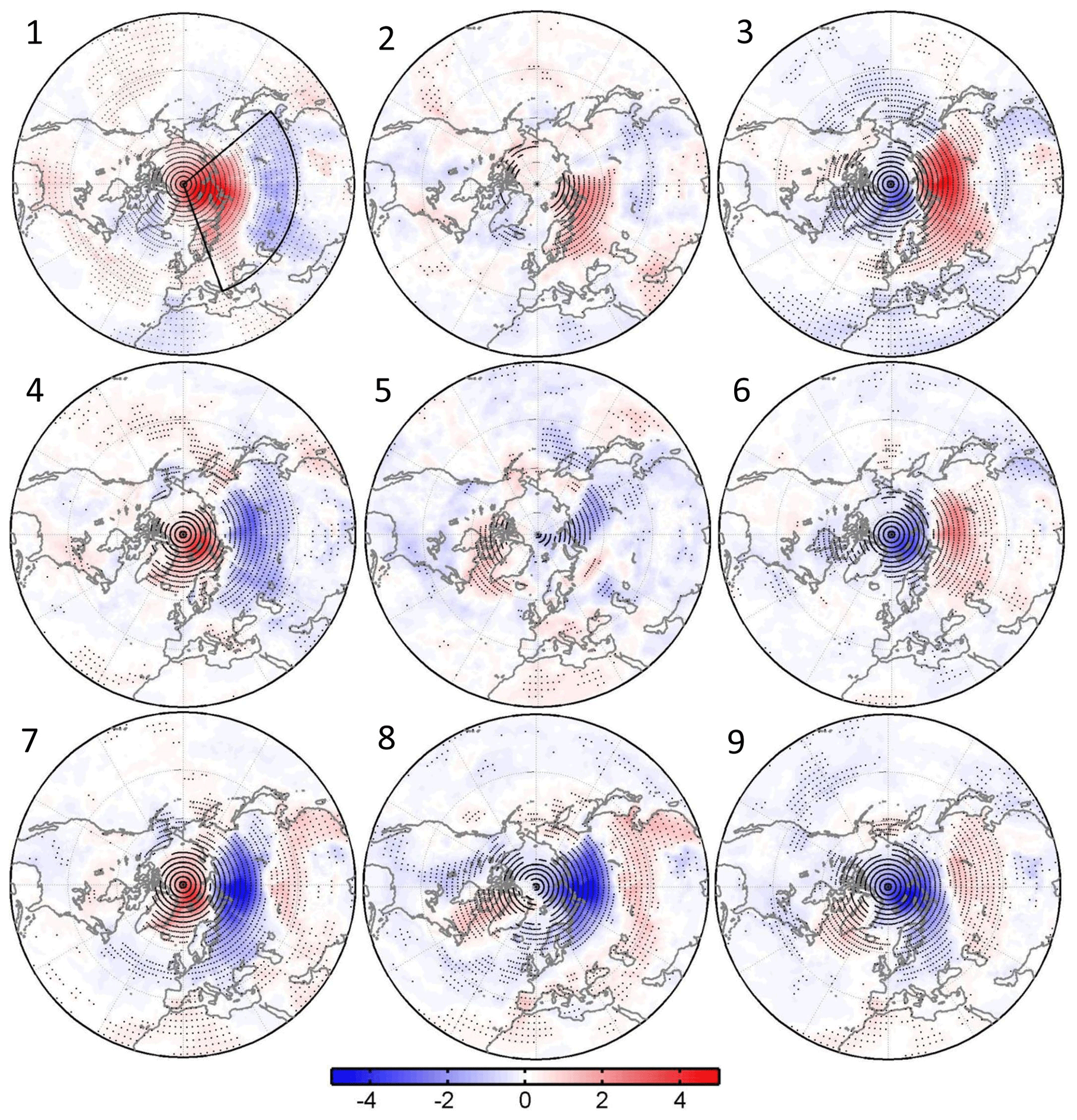
Figure 4Corresponding anomalous daily accumulated downward longwave radiation (105 W m−2) from ERA-Interim reanalysis over the 1979–2019 period for each node in Fig. 1. Dotted regions indicate the above-95 % confidence level.
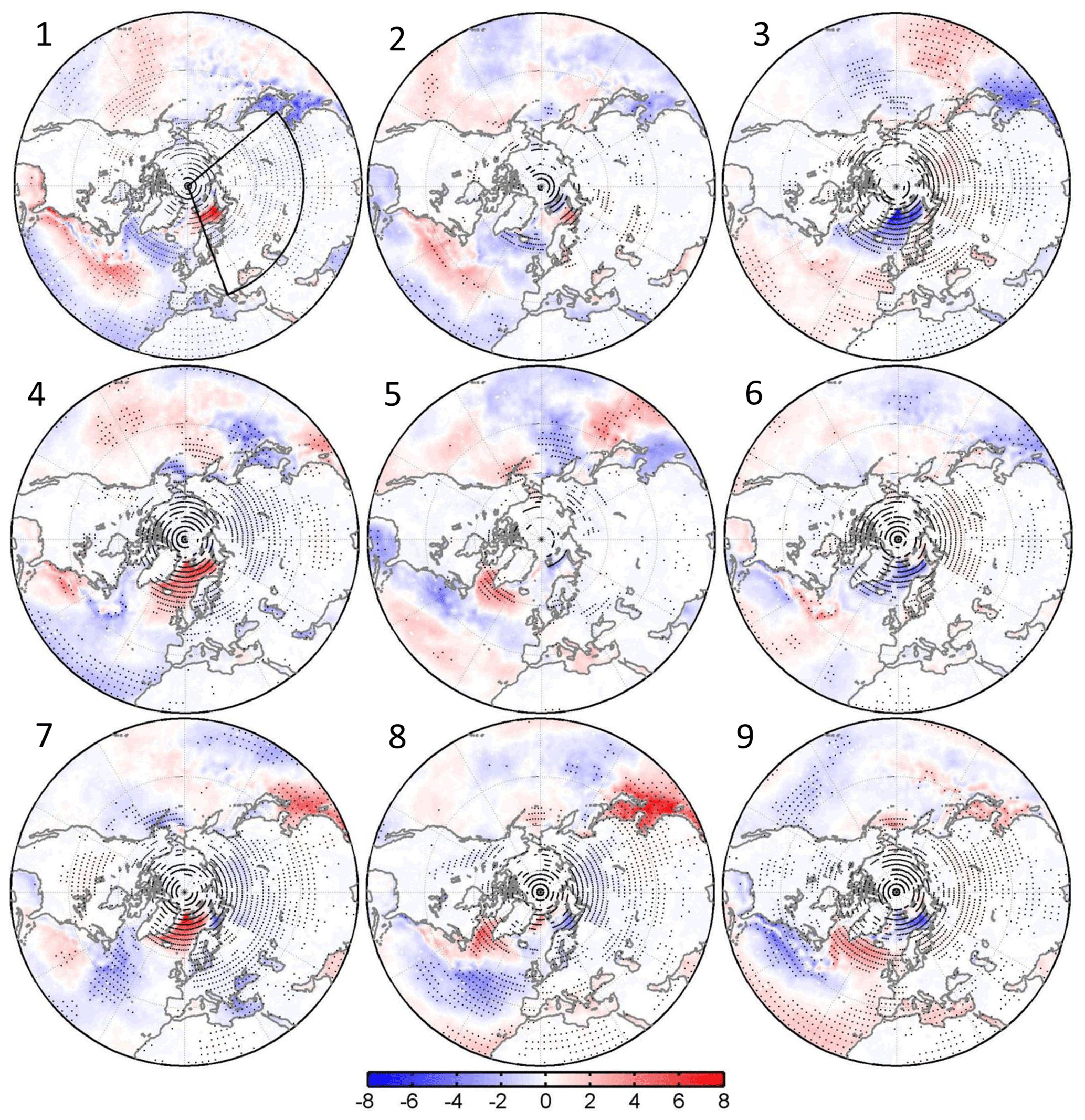
Figure 5Corresponding anomalous daily accumulated turbulent heat flux (sensible and latent heat) (105 W m−2) from ERA-Interim reanalysis over the 1979–2019 period for each node in Fig. 1. Positive values denote heat flux from atmosphere to ocean, and vice versa. Dotted regions indicate the above-95 % confidence level.
3.4 Sea ice
The analyses presented above attempt to explain the spatial pattern of surface temperature variability for each node from the perspective of anomalous heat advection and surface radiative fluxes. As mentioned earlier, there has been a debate in the literature about the role played by the sea ice anomalies in the Barents and Kara seas in the development of the warm Arctic–cold Eurasia pattern. Here, we examine the anomalous turbulent heat flux (Fig. 5) and sea ice concentration (Fig. 6) for each node. Turbulent heat flux is considered positive when it is directed from the atmosphere downward to the ocean or land surfaces. Thus, a positive anomaly indicates either an increase in the atmosphere-to-surface heat transfer or a decrease in the heat transfer from the surface to the atmosphere. The magnitude of anomalous turbulent heat flux is found to be comparable to that of anomalous downward longwave radiation (Fig. 4). For all nodes, the heat flux anomalies are larger over the ocean than over land (Fig. 5). For node 1, positive turbulent heat flux anomalies occur mainly over the Barents Sea, the western and central North Atlantic Ocean, and the eastern North Pacific Ocean, indicating an increase in heat transport from the air to the ocean due possibly to an increase in vertical temperature gradient caused by warm air advection associated with anomalous circulation (Figs. 2 and 3). The downward heat transfer results in sea ice melt in the Greenland Sea and the Barents Sea (Fig. 6). For node 4, the anomalous southerly winds over the Nordic Sea produce larger positive turbulent heat flux anomalies (Fig. 5). For node 7, the anticyclone is located more northwards, which generates opposite anomalous winds between the Nordic and northern Barents seas and the southern Barents Sea and thus opposite turbulent heat flux anomalies that are consistent with the opposite sea ice concentration anomalies in the two regions (Fig. 5). For nodes 3, 6, and 9, the anomalous cold air from the central Arctic Ocean flows into warm water in the Nordic and Barents seas, producing negative turbulent heat flux anomalies and positive sea ice concentration anomalies (Figs. 5 and 6). Sorokina et al. (2016) noted that turbulent heat flux usually peaks 2 d before changes in surface temperature pattern occur. The pattern of the composited anomalous 500 hPa geopotential height, turbulent heat flux, and sea ice concentration 2 d prior to the day when the nodes occur (not shown) is similar to the current-day pattern in Figs. 2, 5, and 6. Our results support the conclusion of Sorokina et al. (2016) and Blackport et al. (2019) that the anomalous atmospheric circulations lead to the anomalous sea ice concentration in the Barents Sea.
3.5 Trends in wintertime surface temperature
The results above suggest that both the surface temperature anomaly patterns over the Arctic Ocean and Eurasian continent and the sea ice concentration anomalies in the Nordic and Barents seas can be explained largely by changes in atmospheric circulations and the associated vertical and horizontal heat and moisture transfer by mean and turbulent flows. Next, we assess the trends of wintertime surface temperature and the contributions of the SOM nodes to the trends.
We first examine the time series of the accumulated number of days for each node in each winter for the 1979–2019 period (Fig. 7). The time series for nodes 1, 4, 6, and 9 exhibit variability on interannual as well as decadal timescales. The occurrence frequency is noticeably larger after 2003 than prior to 2003 for nodes 1 and 4, and vice versa for nodes 6 and 9, and the difference between the two periods is significant at 95 % confidence level. Given the spatial patterns of these four nodes (Fig. 1), this indicates that the warm Arctic–cold Eurasia pattern occurred more frequently after 2003. A linear trend analysis of the time series for each node (Table 3) reveals significant positive trends in occurrence frequency for nodes 1 and 4 and significant negative trends for nodes 6 and 9, which agree with the result from a previous study (Clark and Lee, 2019; Overland et al., 2015) that suggested an increasing trend of the warm Arctic–cold Eurasia pattern.
Table 3Trends in the frequency of occurrences for each SOM node (d yr−1). Asterisks indicate the above-95 % confidence level.

Table 4Frequencies of occurrence (%) of wintertime surface air temperature patterns in Fig. 1 for all winters before 1998 and after 1998 for the period of 1979–2019. Values with asterisks are significantly different from climatology above the 95 % confidence level.

These trends in the occurrence frequency of the SOM nodes contribute to the trends in the total wintertime (December, January, and February; DJF) surface temperature anomalies (Fig. 8a) that have significant positive trends over the Arctic Ocean and in regions of northern and eastern Europe and negative, mostly insignificant trends in central Siberia. The contribution, however, varies from node to node (Fig. 9). Node 1 has the largest domain-averaged contribution of 18.7 %, followed by its mirror node (node 9) at 10.1 %. Nodes 4 and 6 account for 2.8 % and 4.3 % of the total trend, respectively. None of the remaining nodes explain more than 2 %. All nodes together explain 39.5 % of the total trend in wintertime surface air temperature. The spatial pattern of the SOM-explained trends (Fig. 8b) is similar to the warm Arctic–cold continents pattern, whereas the residual trend resembles more the total trend (Fig. 8c).
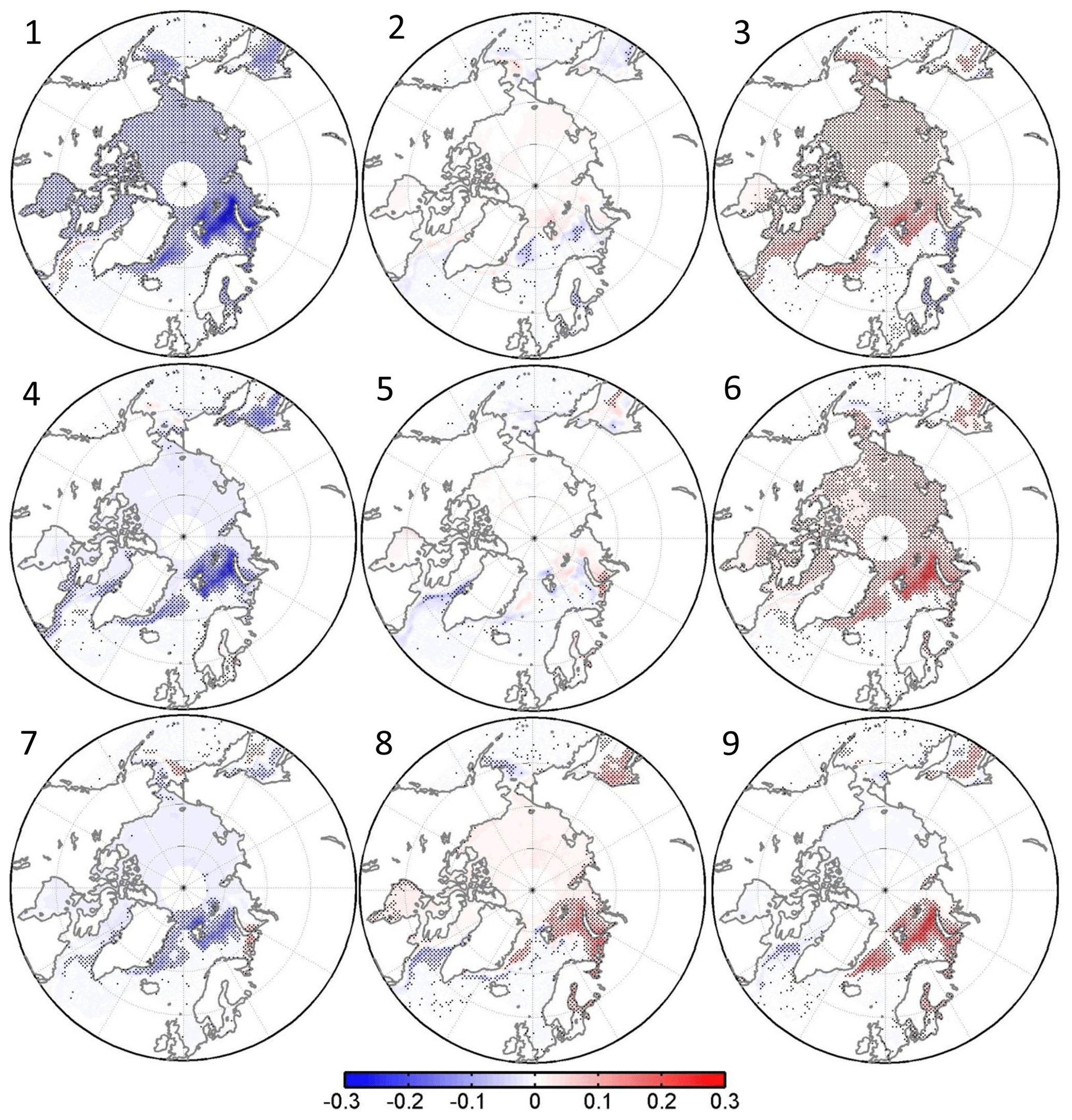
Figure 6Corresponding anomalous wintertime sea ice concentration from the NSIDC over the 1979–2019 period for each node in Fig. 1. Dotted regions indicate the above-95 % confidence level.
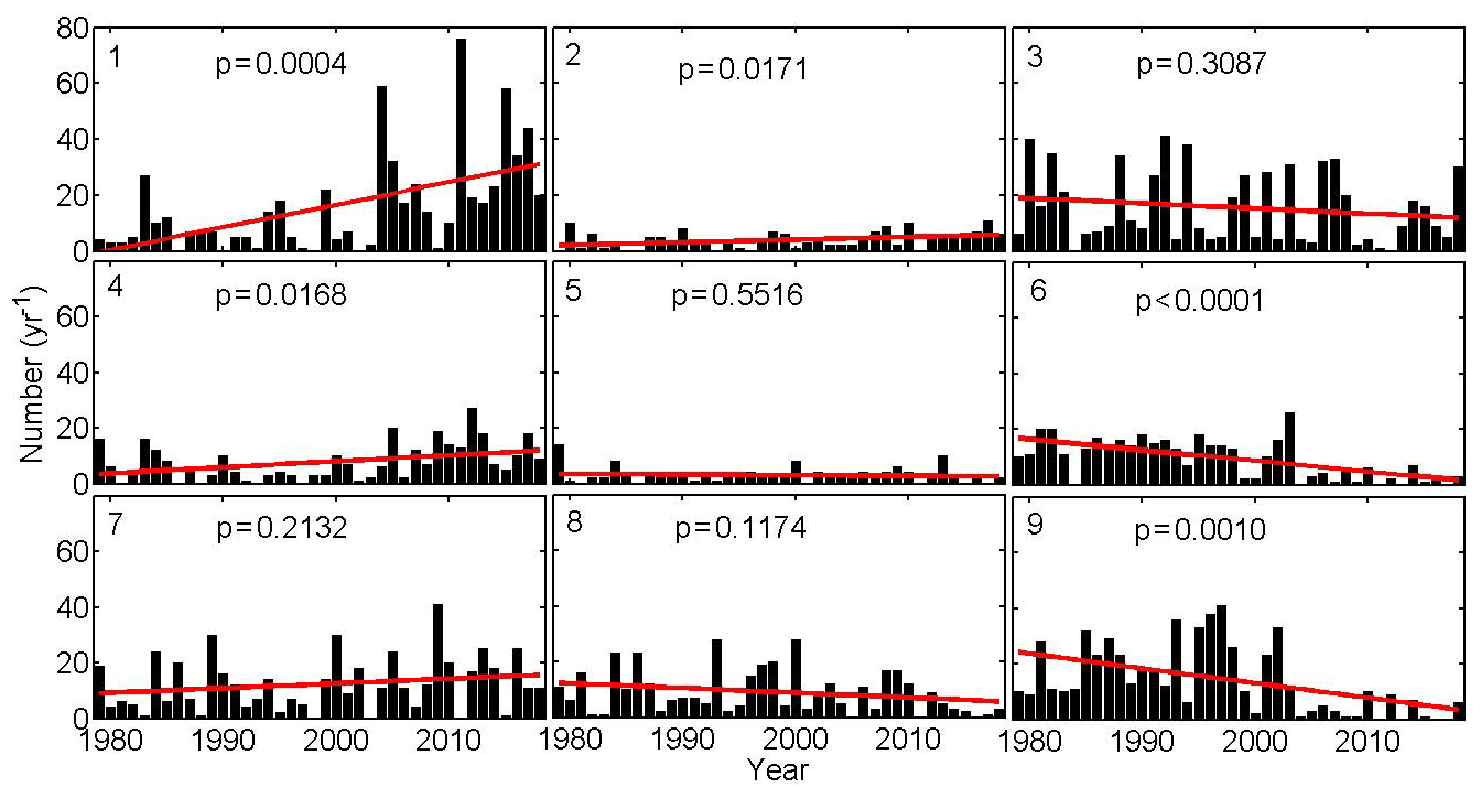
Figure 7Time series of the number of days for occurrence of each SOM node in Fig. 1 over the 1979–2019 period. The red lines denote the trend in the time series.
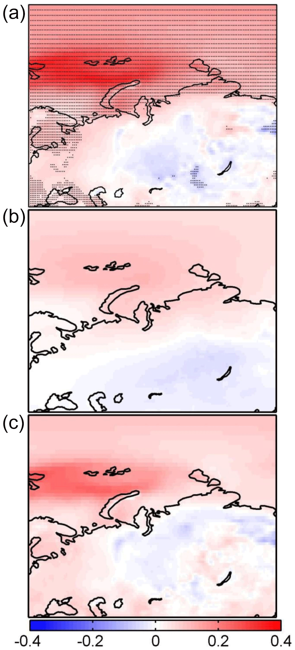
Figure 8Total (a), SOM-explained (b), and residual (c) trend in wintertime (DJF) surface air temperature (∘C yr−1) over the 1979–2019 period. Dots in panel (a) indicate the above-95 % confidence level.
3.6 Mechanisms
The results presented above indicate that the SOM patterns explain nearly 40 % of the trend in wintertime surface air temperature anomalies and majority of the contributions (35 out of 40 %) come from the two pairs of the nodes (nodes 1, 9, and 4, 6). The analyses hereafter will focus on these four nodes. Below, we assess the atmospheric and oceanic conditions associated with the occurrences of the four nodes via regression analysis. Specifically, the anomalous seasonal SST and atmospheric circulation variables are regressed onto the normalized time series of the number of days when each of the four nodes occurs (Figs. 10, 11, and 12).
For node 1, the SST regression pattern in the Pacific Ocean shows significant positive anomalies over the tropical western Pacific Ocean and central North Pacific Ocean (Fig. 10). The positive SST anomalies also occur over most of the North Atlantic. Negative SST anomalies occur over the central tropical Pacific Ocean, though they are not significant at 95 % confidence level. The SST regression pattern is reversed for node 9. The direction of wave activity flux indicates the direction of group speed of stationary planetary wave. Here, we calculate the wave activity flux defined by Takaya and Nakamura (2001), which considers the influence of midlatitude zonal wind (Fig. 12). For node 1, the corresponding anomalous 500 hPa height regression (Fig. 11) shows two Rossby wave trains: one is excited over the central Pacific Ocean and propagates northeastwards into North America and the North Atlantic Ocean, and the other, which displays a stronger signal, originates from central North Atlantic and propagates northeastwards to the Arctic Ocean and southeastwards to the Eurasian continent (Figs. 11 and 12). For node 9, the corresponding anomalous 500 hPa height and streamfunction show an opposite pattern, but the wave activity flux is similar to that of node 1.
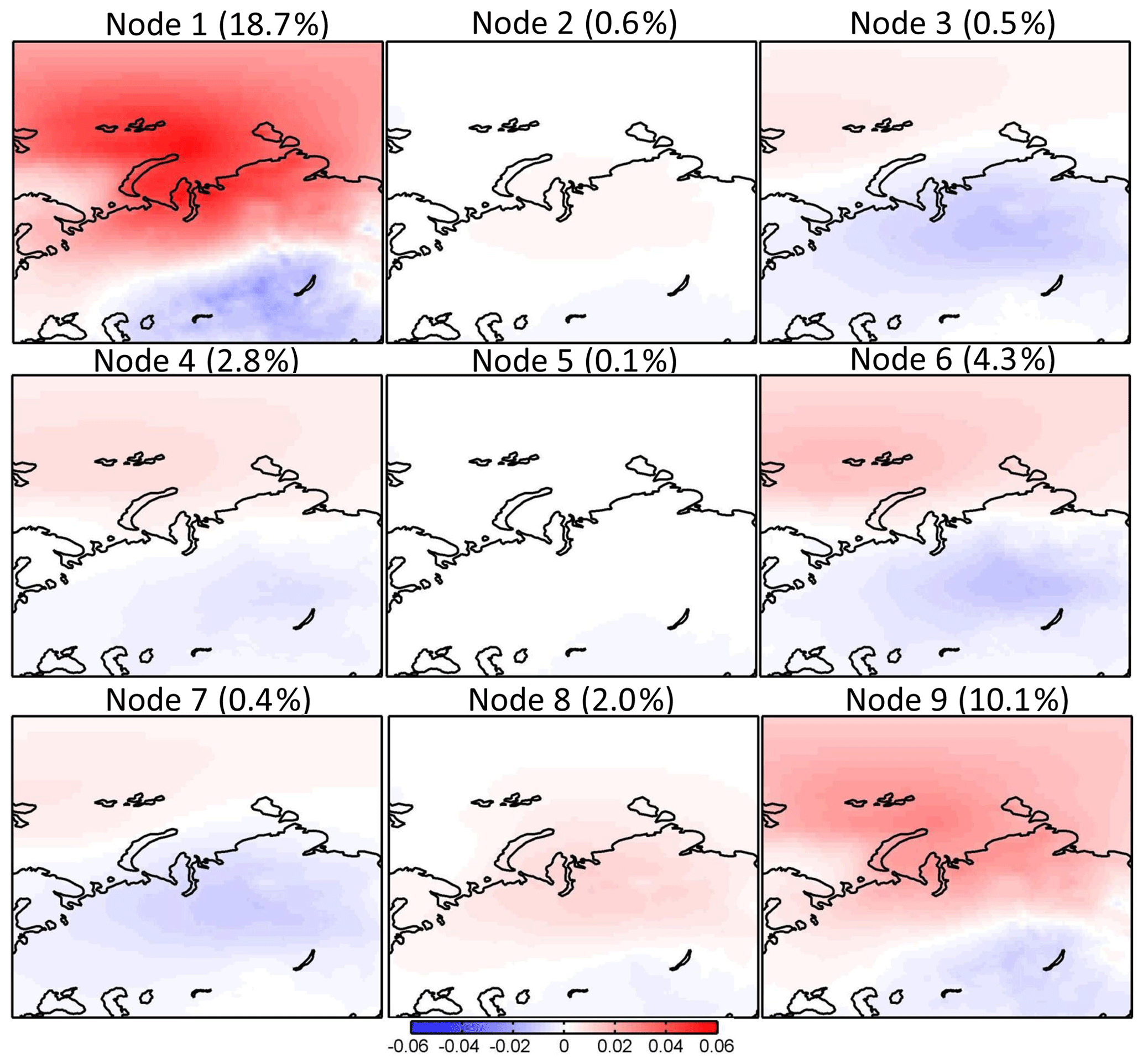
Figure 9Trends in surface air temperature explained by each SOM node (∘C yr−1) over the 1979–2019 period. The percentage in the upper part of each panel indicates the fraction of the total trend represented by each node.
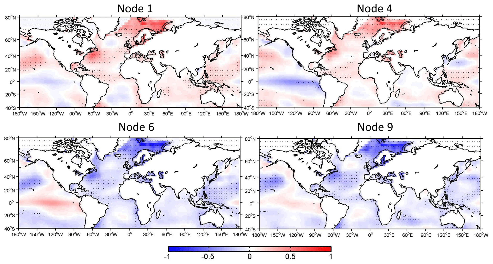
Figure 10Anomalous SST (∘C) from NOAA over the 1979–2019 period regressed into the normalized time series of occurrence number for nodes 1, 4, 6, and 9.
For node 4, the SST anomalies over the tropical Pacific Ocean appear to be in a La Niña state, which shows stronger negative SST anomalies over the eastern tropical Pacific Ocean than those for node 1 (Fig. 10). The positive SST anomalies over the North Pacific shift more northwards relative to that of node 1. The positive SST anomalies over the North Atlantic are weaker than those for node 1. The corresponding wave train over the Pacific Ocean is stronger than that over the Atlantic Ocean (Fig. 11), which is also be observed in the pattern of wave activity and streamfunction (Fig. 12). The corresponding pattern for node 6 is nearly reversed, but there are some noticeable differences in the amplitude of the wave train and SST anomalies. For example, the magnitude of the anomalous SST and the 500 hPa height over the central North Pacific is larger for node 6 than that for node 4.
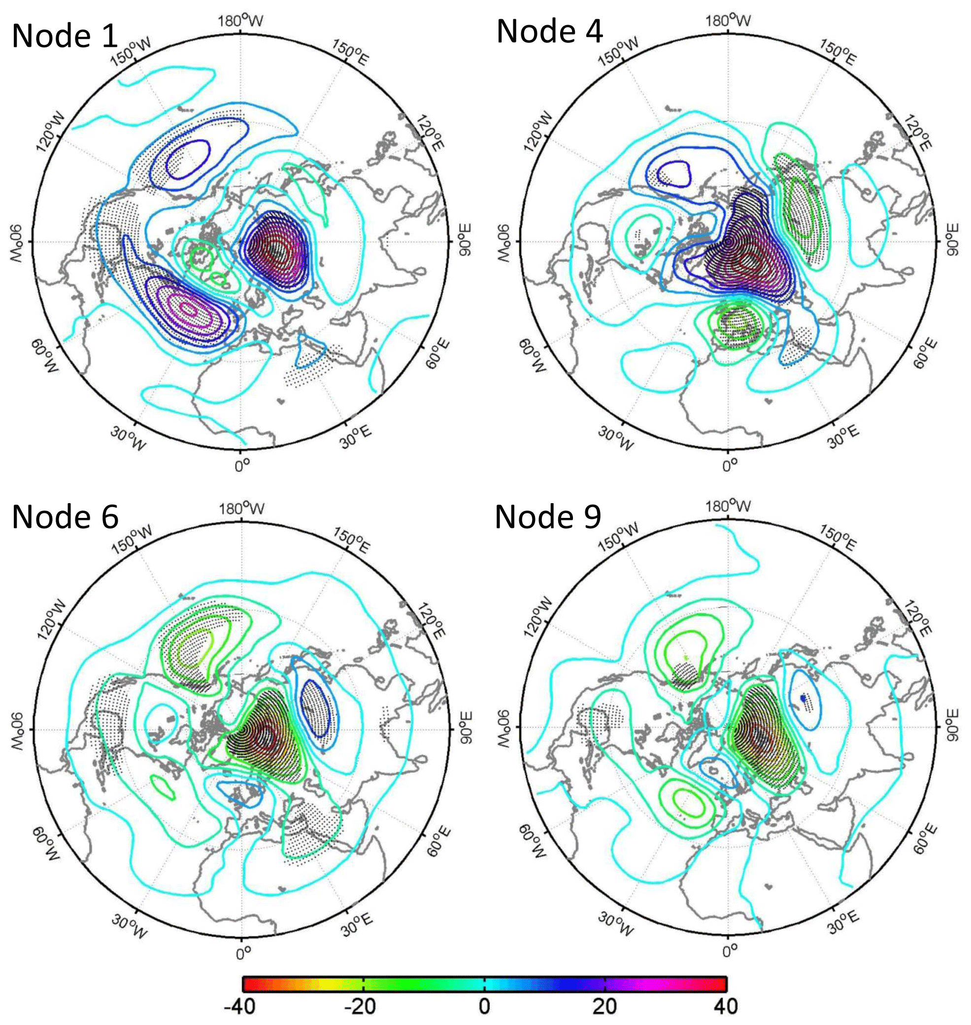
Figure 11Anomalous 500 hPa geopotential height (gpm) from ERA-Interim reanalysis over the 1979–2019 period regressed into the normalized time series of occurrence number for nodes 1, 4, 6, and 9.
Besides the abovementioned variables, similar regression analysis is also performed for the anomalous 850 hPa wind field and anomalous downward longwave radiation (not shown). Their regression patterns, which are similar to those in Figs. 3 and 4, explain well the decadal variability of the number of days for nodes 1, 4, 6, and 9. Together, these results in Figs. 10–12 indicate that the decadal variability of the occurrence frequency of the four nodes in recent decades is related to two wave trains induced by SST anomalies over the central North Pacific Ocean and the North Atlantic Ocean (Figs. 10 and 11). The aforementioned SST regression patterns over the Atlantic and Pacific oceans also show features of the AMO and PDO (Fig. 10). Since both the AMO and PDO exhibited a phase change in the late 1990s (Yu et al., 2017), the question is whether a similar change in the SOM frequency also appears in the late 1990s. A comparison of the averaged frequency before and after 1998 shows a significant drop in frequency for nodes 6 and 9 and an increase in frequency for node 1 (not shown). This result suggests that the change in the AMO and PDO indices may contribute to the change in the frequencies of the warm Arctic–cold Eurasian continent pattern.
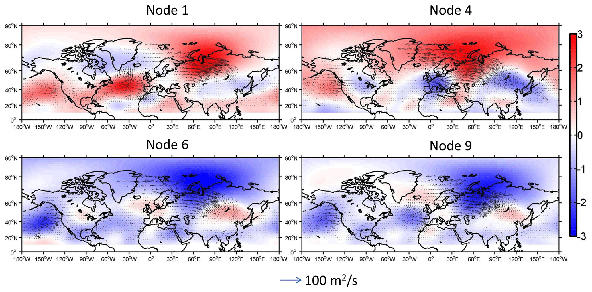
Figure 12The anomalous wave activity flux (vectors) (Takaya and Nakamura, 2001) and stream function (colors, units: 107 m2 s−1) from ERA-Interim reanalysis over the 1979–2019 period regressed onto the normalized time series of occurrence number for nodes 1, 4, 6, and 9.
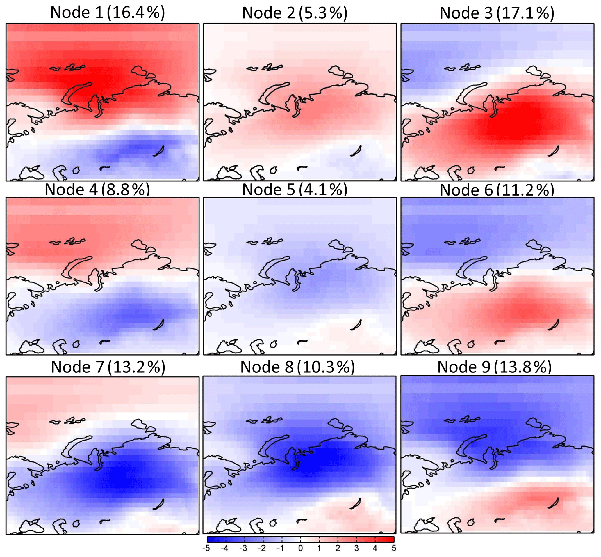
Figure 13Spatial patterns of SOM nodes for detrended daily wintertime (December, January, and February) surface air temperature anomalies (∘C) from the 20CR reanalysis for the 1851–2014 period. The number in brackets denotes the frequency of the occurrence for each node.
3.7 Interdecadal variability
The four-decade-long ERA-Interim reanalysis is not adequate for examining interdecadal to multi-decadal variations represented by the PDO and AMO indices. Further analysis is performed using the 20CR daily reanalysis data for the 1854–2014 period. Before applying the SOM technique to the 20CR data, we first remove the trend to eliminate the influence from the global warming. No low-pass filter is applied before SOM analysis in order to test the stability of the SOM results for the different periods. The spatial SOM patterns from the detrended century-long 20CR data (Fig. 13) are similar to those for the 1979–2019 period (Fig. 1). Nodes 1, 4, and 7 correspond to the positive phase of the warm Arctic–cold Eurasia pattern, and the negative phase can be observed in nodes 3, 6, and 9. The magnitude in Fig. 13 is smaller compared to the recent four decades in Fig. 1. The occurrence frequencies of the four nodes (1, 4, 6, and 9; Fig. 14) are close to those of the recent four decades (Fig. 7). It indicates that the SOM method can obtain stably the main modes of wintertime surface air temperature variability. For the recent four decades, the time series of the number of days also displays a noticeable increasing (decreasing) trend for nodes 1 and 4 (6 and 9), suggesting that the trend in the recent four decades is a reflection of an interdecadal variability of wintertime surface air temperature.
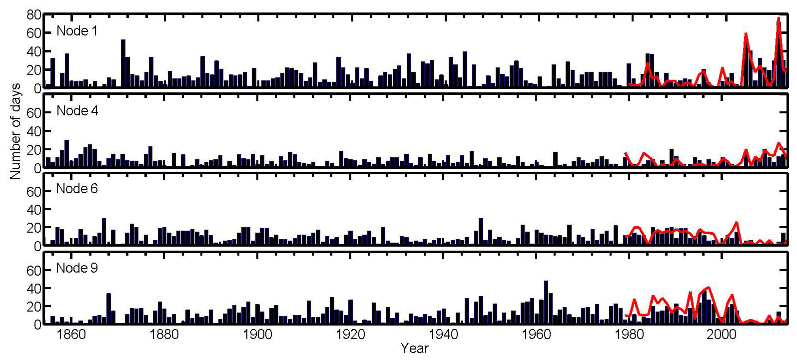
Figure 14Time series of the number of days for occurrence of each SOM node in Fig. 13 from the 20CR reanalysis for the 1851–2014 period. The thick red lines denote the result in Fig. 7 from the ERA-Interim reanalysis for the 1979–2019 period.
Next, we apply a 40-year low-pass filter to the time series of the occurrence frequencies for nodes 1, 4, 6, and 9 and the AMO and PDO indices and calculate correlations. There is a significant correlation between the time series and the AMO index, with correlation coefficients of 0.36 for node 1, 0.27 for node 4, −0.37 for node 6, and −0.20 for node 9, all of which are at the 95 % confidence level. No significant correlations, however, are found between the filtered time series and the PDO index. If we define a SST index to represent the variability of SST anomalies over the central North Pacific Ocean (20–40∘ N, 150∘ E–150∘ W), the 40-year low-pass-filtered central North Pacific Ocean SST index is now significantly correlated with the filtered time series of occurrence frequencies for nodes 1 and 9 (0.55 for node 1 and −0.46 for node 9). The correlation results are consistent with the SST regression map for the recent decades (Fig. 10).
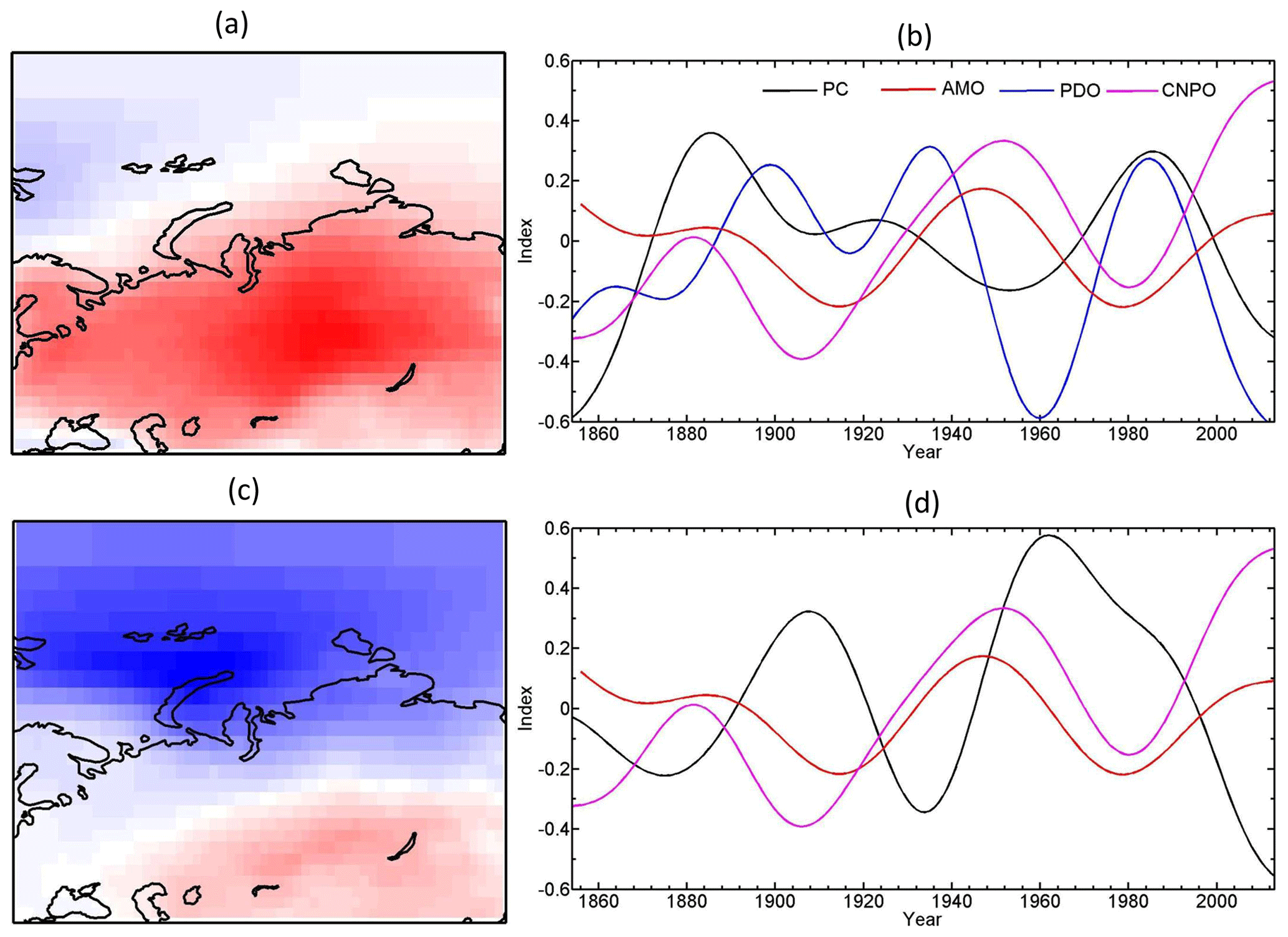
Figure 15The (a) leading pattern and (b) its time series (PC1 and PC2) of EOF analysis of wintertime surface air temperature anomalies from the 20CR reanalysis for the 1851–2014 period. Prior to EOF analysis, surface air temperature data are detrended. A 40-year low-pass filter is applied to the time series of PC1, PC2, AMO, PDO, and central North Pacific Ocean (CNPO) indices. The correlation coefficients between PC1 and AMO, PDO, and CNPO indices are −0.46 (p<0.0001), 0.38 (p<0.0001), and −0.19 (p=0.019); those between PC2 and AMO, PDO, and CNPO indices are −0.44 (p<0.0001), 0.38 (p<0.0001), and −0.26 (p=0.0009).
To confirm the effect of SST anomalies on the warm Arctic–cold Eurasia pattern, we also perform EOF analysis of wintertime detrended seasonal surface air temperature anomalies for the 1854–2014 period (Fig. 15). The spatial patterns of the first and second EOF modes show the negative phase of the warm Arctic–cold Eurasia pattern and the 40-year low-pass-filtered time series is inversely correlated with the 40-year low-pass-filtered wintertime AMO index (−0.46, p<0.05 for mode 1 and −0.44, p<0.05 for mode 2). The 40-year low-pass-filtered time series of the two EOF modes have a significant negative correlation with the 40-year low-pass-filtered central North Pacific Ocean SST index, with correlation coefficients of −0.19 and −0.26 (p<0.05). Only PC1 has a significant correlation with the PDO index (0.38, p<0.05). Thus, the increase in the occurrence of the warm Arctic–cold Eurasia pattern in the recent decades is a part of the interdecadal variability of the pattern, which is influenced by the AMO index, the PDO index, and the central North Pacific SST.
In this study, we examine the variability of wintertime surface air temperature in the Arctic and the Eurasian continent (20–130∘ E) by applying the SOM method to daily temperature from the gridded ERA-Interim dataset for the period of 1979–2019 and from the 20CR reanalysis for the period of 1854–2014 and the EOF method to seasonal temperature from the 20CR reanalysis for the period of 1854–2014. The spatial pattern in the surface temperature variations in the study region, as revealed by the nine SOM nodes, is dominated by concurrent warming in the Arctic and cooling in Eurasia, and vice versa. The nine SOM patterns explain nearly 40 % of the trends in wintertime surface temperature and 88 % of that are accounted for by only four nodes. Two of the four nodes (nodes 1 and 4) represent the warm Arctic–cold Eurasia pattern and the other two (nodes 6 and 9) depict the opposite cold Arctic–warm Eurasia pattern. There is a clear shift in the frequency of the occurrence of these patterns near the beginning of this century, with the warm Arctic–cold Eurasia pattern dominating since 2003, while the opposite pattern has been prevailing from the 1980s to the 1990s. The warm Arctic–cold Eurasia pattern is accompanied by an anomalous high pressure and anticyclonic circulation over the Eurasian continent. The anomalous winds and the associated temperature and moisture advection interact with local longwave radiative forcing and turbulent fluxes to produce positive (negative) temperature anomalies in the Arctic (Eurasian continent). The circulation is reversed for the cold Arctic–warm Eurasia pattern. The warm, moist air mass is advected to the Arctic by the anomalous atmospheric circulations, and the increased downward turbulent heat flux also explains sea ice melt in the Barents and Kara seas. In other words, the sea ice loss in the Barents and Kara seas and the cooling of the Eurasian continent can both be traced to anomalous atmospheric circulations.
Increasing occurrences of the warm Arctic–cold Eurasian continent pattern appear to relate to rising SST over the central North Pacific and North Atlantic oceans (positive AMO phase). The SST anomalies trigger two Rossby wave trains spanning from the North Pacific Ocean, North America, and the North Atlantic Ocean to the Eurasian continent. The two wave trains are strengthened through local sea–atmosphere–ice interactions in mid-to-high latitudes, which influence the change in the occurrence frequency of the warm Arctic–cold Eurasian continent pattern. Our results agree with those of previous studies (Lee et al., 2011; Sato et al., 2014; Clark and Lee, 2019). But previous studies only focus on the effects of SST anomalies over either the North Pacific or North Atlantic oceans. We also note that the two wave trains excited by SST anomalies over different oceans differ in amplitudes, leading to somewhat different warm Arctic–cold Eurasia patterns.
Using century-long data, we show that the warm Arctic–cold Eurasia pattern is an intrinsic climate mode, which has been stable since 1854. The recent increasing trend in its occurrence is a reflection of an interdecadal variability of the pattern resulting from the interdecadal variability of SST anomalies over the central Pacific Ocean and over the Atlantic Ocean represented by the AMO index. Sung et al. (2018) investigated interdecadal variability of the warm Arctic–cold Eurasia pattern and considered the variability of the SST over the North Atlantic as its origin. Our results suggest that the variability of the SST over the North Pacific also plays an important role. However, internal atmospheric variability remains another potential source. The Rossby wave trains also lead to the deepening of a trough in East Asia and generate an anomalous low pressure and cold temperature in northern China (Fig. 10), which further suggests that a warmer Arctic, especially warmer Barents and Kara seas, is not the driver for the increasing occurrence of cold spells in East Asia, as suggested in previous studies (Kim et al., 2014; Mori et al., 2014; Kug et al., 2015; Overland et al., 2015).
Our results suggest that the increasing trend in warm Arctic–cold Eurasia pattern may be related to the anomalous SST over the central North Pacific and the North Atlantic oceans. But we cannot rule out the influence of the Arctic sea ice loss on the trend. The Arctic sea ice loss results from both Arctic warming due to anthropogenic increasing of greenhouse gas concentrations and natural variability of climate system such as SST anomalies. This study considers natural variability or internal driver of climate system. The Arctic warming caused external forcing related to increasing greenhouse gas emissions can produce an anomalous anticyclone over the Barents and Kara seas, leading to the warm Arctic–cold continents pattern.
Although the ERA-Interim reanalysis is overall superior in describing the Arctic atmospheric environment to other similar global reanalysis products, it contains warm and moist biases in the surface layer (Jakobson et al., 2012; Chaudhuri et al., 2014; Simmons and Poli, 2015; Wang et al., 2019). However, we believe these biases, as well as the relatively coarse resolution, should have minimum impact in the results from the current analyses. Further, although the current analyses were performed on a predetermined SOM grid with 3×3 nodes, an increase in the number of SOM nodes did not change the conclusions.
Our results help broaden the current understanding of the formation mechanisms for the warm Arctic–cold Eurasia pattern. The SST anomalies over Northern Hemisphere oceans may offer a potential for predicting its occurrence. The statistical relationship between SST anomalies and the occurrences of the warm Arctic–cold continents pattern may help improve the predictability of wintertime surface air temperature over Eurasian continent on interdecadal timescales.
All data used in the current analyses are publicly available. The monthly sea ice concentration data are available from NSIDC (http://nsidc.org/data/NSIDC-0051, last access: 31 August 2020, Cavalieri et al., 1996), the ERA-Interim reanalysis data are available from the ECMWF (https://www.ecmwf.int/en/forecasts/datasets/reanalysis-datasets/era-interim, last access: 31 August 2020, Dee et al., 2011) and the sea surface temperature data are available from the Hadley Centre for Climate Prediction and Research (ftp://ftp.cdc.noaa.gov/Datasets/noaa.oisst.v2.highres/, last access: 29 September 2020, Rayner et al., 2003). The long-term SST data are derived from the 20th Century Reanalysis project, version 2c (20CR) (https://climatedataguide.ucar.edu/climate-data/noaa-20th-century-reanalysis-version-2-and-2c, last access: 13 April 2020, Compo et al., 2011).
LY designed the study, with input from SZ, and carried out the analyses. LY and SZ prepared the manuscript. CS plotted part of figures. BS revised the manuscript.
The authors declare that they have no conflict of interest.
We thank the European Centre for Medium-Range Weather Forecasts (ECMWF) for the ERA-Interim data.
This study is financially supported by the National Key R&D Program of China (grant nos. 2017YFE0111700; 2019YFC1509102) and the National Natural Science Foundation of China (grant nos. 41922044; 41976221).
This paper was edited by Patrick Jöckel and reviewed by two anonymous referees.
Barnes, E. A. and Screen, J. A.: The impact of Arctic warming on the midlatitude jet-stream: Can it? Has it? Will it?, WIRES Clim. Change, 6, 277–286, https://doi.org/10.1002/wcc.337, 2015.
Blackport, R., Screen J. A., van der Wiel K., and Bintanja, R.: Minimal influence of reducedArctic sea ice on coincident cold winters in mid-latitudes, Nat. Clim. Change, 9, 697–704, https://doi.org/10.1038/s41558-019-0551-4, 2019.
Cavalieri, D. J., Parkinson, C. L., Gloersen, P., and Zwally, H. J.: updated yearly. Sea Ice Concentrations from Nimbus-7 SMMR and DMSP SSM/I-SSMIS Passive Microwave Data, Version 1, NASA National Snow and Ice Data Center Distributed Active Archive Center, Boulder, Colorado USA, https://doi.org/10.5067/8GQ8LZQVL0VL, 1996.
Chaudhuri, A. H., Ponte, R. M., and Nguyen, A. T.: A Comparison of atmospheric reanalysis products for the Arctic Ocean and implications for uncertainties in air-sea fluxes, J. Climate, 27, 5411–5421, https://doi.org/10.1175/JCLI-D-13-00424.1, 2014.
Chen, L., Francis J., and Hanna E.: The “Warm-Arctic/Cold continents” pattern during 1901–2010, Int. J. Climatol., 38, 5245–5254, https://doi.org/10.1002/joc.5725, 2018.
Clark, J. P. and Lee, S.: The role of the tropically excited Arctic Warming Mechanism on the warm Arctic cold continent surface air temperature trend pattern, Geophys. Res. Lett., 46, 8490–8499, https://doi.org/10.1029/2019GL082714, 2019
Cohen, J., Screen, J. A., Furtado, J. C., Barlow, M., Whittleston, D., Coumou, D., Francis, J., Dethloff, K., Entekhabi, D., Overland, J., and Jones, J.: Recent Arctic amplification and extreme mid-latitude weather, Nat. Geosci., 7, 627–637, https://doi.org/10.1038/ngeo2234, 2014.
Cohen, J., Pfeiffer, K., and Francis, J. A.: Warm Arctic episodes linked with increased frequency of extreme winter weather in the United States, Nat. Commun., 9, 869, https://doi.org/10.1038/s41467-018-02992-9, 2018.
Compo, G. P., Whitaker, J. S., Sardeshmukh, P. D., Matsui, N., Allan, R., Yin, X., Jr, G. B. E., Vose, R. S., Rutledge, G. K., Bessemoulin, P., Brönnimann, S., Brunet, M., Crouthamel, R. I., Grant, A. N., Groisman, P. Y., Jones, P. D., Kruk, M. C., Kruger, A. C., Marshall, G. J., Maugeri, M., Mok, H. Y., Nordli, Ø., Ross, T. F., Trigo, R. M., Wang, X., Woodruff, S. D., and Worley S. J.: The Twentieth Century Reanalysis Project, Q. J. Roy. Meteor. Soc., 137, 1–28, https://doi.org/10.1002/qj.776, 2011.
Dee, D. P., Uppala, S. M., Simmons, A. J., Berrisford, P., Poli, P., Kobayashi, S., Andrae, U., Balmaseda, M. A., Balsamo, G., Bauer, P., Bechtold, P., Beljaars, A. C. M., van de Berg, I., Biblot, J., Bormann, N., Delsol, C., Dragani, R., Fuentes, M., Greer, A. J., Haimberger, L., Healy, S. B., Hersbach, H., Holm, E. V., Isaksen, L., Kallberg, P., Kohler, M., Matricardi, M., McNally, A. P., Mong-Sanz, B. M., Morcette, J.-J., Park, B.-K., Peubey, C., de Rosnay, P., Tavolato, C., Thepaut, J. N., and Vitart, F.: The ERA-Interim reanalysis: Configuration and performance of the data assimilation system, Q. J. Roy. Meteorol. Soc., 137, 553–597, https://doi.org/10.1002/qj.828, 2011.
Enfield, D. B., Mestas-Nunez, A. M., and Trimble, P. J.: The Atlantic multidecadal oscillation and it's relation to rainfall and river flows in the continental U.S., Geophy. Res. Lett., 28, 2077–2080, 2001.
Fyfe, J. C.: Midlatitudes unaffected by sea ice loss, Nat. Clim. Change, 9, 649–650, https://doi.org/10.1038/s41558-019-0560-3, 2019.
Gibson, P. B., Perkins-Kirkpatrick, S. E., Uotila, P., Pepler, A. S., and Alexander, L. V.: On the use of self-organizing maps for studying climate extremes, J. Geophys. Res.-Atmos., 122, 3891–3903, https://doi.org/10.1002/2016JD026256, 2017.
Horton, D. E., Johnson, N. C., Singh, D., Swain, D. L., Rajaratnam, B., and Diffenbaugh, N. S.: Contribution of changes in atmospheric circulation patterns to extreme trends, Nature, 522, 465–469, https://doi.org/10.1038/nature14550, 2015.
Hoskins, B. and Woollings, T.: Pesistent extratropical regims and climate extremes, Curr. Clim. Change Rep., 1, 115–124, https://doi.org/10.1007/s40641-015-0020-8, 2015
Inoue, J., Hori, M. E., and Takaya, K.: The role of Barents Sea ice in the wintertime cyclone track and emergence of a warm-Arctic-Siberian anomaly, J. Clim., 25, 2561–2568, https://doi.org/10.1175/JCLI-D-11-00449.1, 2012.
Jakobson, E., Vihma, T., Palo, T., Jakobson, L., Keernik, H., and Jaagus, J.: Validation of atmospheric reanalyses over the central Arctic Ocean, Geophys. Res. Lett., 39, L10802, https://doi.org/10.1029/2012GL051591, 2012.
Johnson, N. C. and Feldstein, S. B.: The continuum of North Pacific sea level pressure patterns: Intraseasonal, interannual, and interdecadal variability, J. Clim., 23, 851–867, https://doi.org/10.1175/2009JCLI3099.1, 2010.
Kalnay, E., Kanamitsu, M., Kistler, R., Collins, W. G., Deaven, D., Gandin, L., Iredell, M., Saha, S., White, G., and Woollen J.: The NCEP/NCAR 40-year reanalysis project, B. Am. Meteorol. Soc., 77, 437–471, https://doi.org/10.1175/1520-0477(1996)077<0437:TNYRP>2.0.CO;2, 1996.
Kim, B.-M., Son, S.-W., Min, S.-K., Jeong, J.-H., Kim, S.-J., Zhang, X., Shim, T., and Yoon, J.-H.: Weakening of the stratospheric polar vortex by Arctic sea-ice loss, Nat. Commun., 5, 4646, https://doi.org/10.1038/ncomms5646, 2014.
Kohonen, T.: Self-Organizing Maps, 3rd edn., Springer, 501 pp., 2001.
Kug, J.-S., Jeong, J.-H., Jang, Y.-S., Kim, B.-M., Folland, C. K., Min, S.-K., and Son, S.-W.: Two distinct infleunces of Arctic warming on cold winters over North America and East Asia, Nat. Geosci., 8, 759–762, https://doi.org/10.1038/ngeo2517, 2015.
Lee, S., Gong, T., Johnson, N., Feldstein, S. B., and Polland, D.: On the possible link between tropical convection and the Northern Hemisphere Arctic surface air temperature change between 1958 and 2001, J. Clim., 24, 4350–4367, https://doi.org/10.1175/2011JCLI4003.1, 2011.
Lee, S. and Feldstein, S. B.: Detecting ozone- and greenhouse gas–driven wind trends with observational data, Science, 339, 563–567, https://doi.org/10.1126/science.1225154, 2013.
Loikith, P. C. and Broccoli, A. J.: Comparison between observed and model-simulated atmospheric circulation patterns associated with extreme temperature days over North America using CMIP5 historical simulations, J. Clim., 28, 2063–2079, https://doi.org/10.1175/JCLI-D-13-00544.1, 2015.
Luo, D., Xiao, Y., Yao, Y., Dai, A., Simmonds, I., and Franzke, C. L. E.: Impact of Ural blocking on winter warm Arctic-cold Eurasian anomalies. Part I: Blocking-induced amplification, J. Clim., 29, 3925–3947, https://doi.org/10.1175/JCLI-D-15-0611.1, 2016.
Mantua, N. J., Hare, S. R., Zhang, Y., Wallace, J. M., and Francis, R. C.: A Pacific interdecadal climate oscillation with impacts on salmon production, B. Am. Meteorol. Soc., 78, 1069–1079, 1997.
Matsumura, S. and Kosaka, Y.: Arctic-Eurasian climate linkage induced by tropical ocean variability, Nat. Commun., 10, 3441, https://doi.org/10.1038/s41467-019-11359-7, 2019.
McCusker, K. E., Fyfe, J. C., and Sigmond, M.: Twenty-five winters of unexcepted Eurasian cooling unlikely due to Arctic sea-ice loss, Nat. Geosci., 9, 838–842, https://doi.org/10.1038/ngeo2820, 2016.
Mori, M., Watanabe, M., Shiogama, H., Inoue, J., and Kimoto, M.: Robust Arctic sea-ice influence on the frequent Eurasian cold winters in past decades, Nat. Geosci., 7, 869–873, https://doi.org/10.1038/ngeo2277, 2014.
Mori, M., Kosaka, Y., Watanabe, M., Nakamura, H., and Kimoto, M.: A reconciled estimate of the influence of Arctic sea-ice loss on recent Eurasian cooling, Nat. Clim. Change, 9, 123–129, https://doi.org/10.1038/s41558-018-0379-3, 2019.
Overland, J. E., Wood, K. R., and Wang, M.: Warm Arctic-cold continents: climate impacts of the newly open Arctic sea, Polar Res., 30, 15787, https://doi.org/10.3402/polar.v30i0.15787, 2011.
Overland, J. E., Francis, J., Hall, R., Hanna, E., Kim, S.-J., and Vihma, T.: The melting Arctic and Midlatitude weather patterns: Are they connected?, J. Clim., 28, 7917–7932, https://doi.org/10.1175/JCLI-D-14-00822.1, 2015.
Palmer, T. N.: A nonlinear dynamical perspective on climate prediction, J. Clim., 12, 575–591, 1999. https://doi.org/10.1175/1520-0442(1999)012< 0575:ANDPOC>2.0.CO;2
Peings, Y.: Ural blocking as a driver of early-winter stratospheric warmings, Geophys. Res. Lett., 46, 5460–5468, https://doi.org/10.1029/2019GL082097, 2019.
Rayner, N. A., Parker, D. E., Horton, E. B., Folland, C. K., Alexander, L. V., Rowell, D. P., Kent, E. C., and Kaplan, A.: Global analyses of sea surface temperature, sea ice, and night marine air temperature since the late nineteenth century, J. Geophys. Res., 108, 4407, https://doi.org/10.1029/2002JD002670, 2003.
Reusch, D. B., Alley, R. B., and Hewitson, B. C.: Relative performance of self-organizing maps and principal component analysis in pattern extraction from synthetic climatological data, Polar Geogr., 29, 188–212, https://doi.org/10.1080/789610199, 2005.
Reynolds, R. W., Smith, T. M., Liu, C., Chelton, D. B., Casey, K. S., and Schlax, M. G.: Daily High-Resolution-Blended Analyses for Sea Surface Temperature, J. Climate, 20, 5473–5496, https://doi.org/10.1175/2007JCLI1824.1, 2007.
Sammon, J. W.: A non-linear mapping for data structure analysis, IEEE Trans. Computers, C-18, 401–409, 1969.
Sato, K., Inoue, J., and Watanabe, M.: Influence of the Gulf Stream on the Barents Sea ice retreat and Eurasian coldness during early winter, Environ. Res. Lett., 9, 084009, https://doi.org/10.1088/1748-9326/9/8/084009, 2014.
Schudeboom, A., McDonald, A. J., Morgenstern, O., Harvey, M., and Parsons, S.: Regional regime-based evaluation of present-day GCM cloud simulations using self-organizing maps, J. Geophys. Res.-Atmos., 123, 4259–4272, https://doi.org/10.1002/2017JD028196, 2018.
Screen, J. A. and Simmonds, I.: The central role of diminishing sea ice in recent Arctic temperature amplification, Nature, 464, 1334–1337, https://doi.org/10.1038/nature09051, 2010.
Screen, J. S. and Simmonds, I.: Erroneous Arctic temperature trends in the ERA-40 reanalysis: A closer look, J. Clim., 24, 2620–2627, https://doi.org/10.1175/2010JCLI4054.1, 2011.
Sedlar, J., Tjernström, M., Mauritsen, T., Shupe, M. D., Brooks, I. M., Persson, O., Birch, C. E., Leck, C., Sirevaag, A., and Nicolaus, M.: A transitioning Arctic surface energy budget: The impacts of solar zenith angle, surface albedo and cloud radiative forcing, Clim. Dyn., 37, 1643–1660, https://doi.org/10.1007/s00382-010-0937-5, 2011.
Shepherd, T. G.: Effects of a warming Arctic, Science, 353, 989–990, https://doi.org/10.1126/science.aag2349, 2016.
Simmons, A. and Poli, P.: Arctic warming in ERA-Interim and other analyses, Q. J. R. Meteor. Soc., 141, 1147–1162, https://doi.org/10.1002/qj.2422, 2015.
Skific, N., Francis, J. A., and Cassano, J. J.: Attribution of projected changes in atmospheric moisture transport in the Arctic: A self-organizing map perspective, J. Clim., 22, 4135–4153, https://doi.org/10.1175/2009JCLI2645.1, 2009.
Sorokina, S. A., Li, C., Wettstein, J. J., and Kvamstø, N. G.: Observed atmospheric coupling between Barents sea ice and the warm-Arctic cold-Siberian anomaly pattern, J. Clim., 29, 495–511, https://doi.org/10.1175/JCLI-D-15-0046.1, 2016.
Stroeve, J. C.: Trends in Arctic sea ice extent from CMIP5, CMIP3 and observations, Geophys. Res. Lett., 39, L16502, https://doi.org/10.1029/2012GL052676 , 2012.
Stroeve, J. C., Holland, M. M., Meier, W., Scambos, T., and Serreze, M.: Arctic sea ice decline: faster than forecast, Geophys. Res. Lett., 34, L09051, https://doi.org/10.1029/2007gl029703, 2007.
Sun, L., Perlwitz, J., and Hoerling, M.: What caused the recent “warm Arctic-Cold Continents” trend pattern in winter temperature?, Geophys. Res. Lett., 43, 5345–5352, https://doi.org/10.1002/2016GL069024, 2016.
Sung, M.-K., Kim, S.-H., Kim, B.-M., and Choi, Y.-S.: Interdecadal variability of the warm Arctic and cold Eurasia pattern and its North Atlantic origin, J. Clim., 31, 5793–5810, https://doi.org/10.1175/JCLI-D-17-0562.1, 2018.
Takaya, K., and Nakamura, H.: A formulation of a phase-independent wave-activity flux for stationary and migratory quasigeostrophic eddies on a zonally varying basic flow, J. Atmos. Sci., 58, 608–627, 2001.
Tang, Q., Zhang, X., Yang, X., and Francis J. A.: Cold winter extremes in northern conditions linked to Arctic sea ice loss, Environ. Res. Lett., 8, 014036, https://doi.org/10.1088/1748-9326/8/1/014036, 2013.
Uppala, S. M., Kållberg, P. W., Simmons, A. J., Andrae, U., Da Costa Bechtold, V., Fiorino, M., Gibson, J.K., Haseler, J., Her- nandez, A., Kelly, G. A., Li, X., Onogi, K., Saarinen, S., Sokka, N., Allan, R. P., Anderson, E., Arpe, K., Balmaseda, M. A., Beljaars, A. C. M., Van De Berg, L., Bidlot, J., Bormann, N., Caires, S., Chevallier, F., Dethof, A., Dragosavac, M., Fisher, M., Fuentes, M., Hagemann, S., Hólm, E., Hoskins, B. J., Isaksen, L., Janssen, P. A. E. M., Jenne, R., Mcnally, A. P., Mahfouf, J.-F., Morcrette, J.-J., Rayner, N. A., Saunders, R. W., Simon, P., Sterl, A., Trenbreth, K. E., Untch, A., Vasiljevic, D., Viterbo, P., and Woollen, J.: The ERA-40 re-analysis, Q. J. Roy. Meteor. Soc., 131, 2961–3012, https://doi.org/10.1256/qj.04.176, 2005.
Walsh, J. E.: Intensified warming of the Arctic: Causes and impacts on middle Latitudes, Glob. Planet. Change, 117, 52–63, https://doi.org/10.1016/j.gloplacha.2014.03.003, 2014.
Vihma, T.: Effects of Arctic sea ice decline on weather and climate: A review, Surv. Geophys., 35, 1175–1214, https://doi.org/10.1007/s10712-014-9284-0, 2014.
Vihma, T., Graversen, R., Chen, L., Handorf, D., Skific, N., Francis, J. A., Tyrrell, N., Hall, R., Hanna, E., Uotila, P., Dethloff, K., Karpechko, A. Y., Björnsson, H., and Overland, J. E.: Effects of the tropospheric large-scale circulation on European winter temperatures during the period of amplified Arctic warming, Int. J. Climatol., 40, 509–529, https://doi.org/10.1002/joc.6225, 2019.
Wang, C., Graham, R. M., Wang, K., Gerland, S., and Granskog, M. A.: Comparison of ERA5 and ERA-Interim near-surface air temperature, snowfall and precipitation over Arctic sea ice: effects on sea ice thermodynamics and evolution, The Cryosphere, 13, 1661–1679, https://doi.org/10.5194/tc-13-1661-2019, 2019.
Yoo, C., Feldstein, S., and Lee, S.: The impact of the Madden–Julian oscillation trend on the Arctic amplification of surface air temperature during the 1979–2008 boreal winter, Geophys. Res. Lett., 38, L24804, https://doi.org/10.1029/2011GL049881, 2011.
Yu, L., Zhong, S., Winkler, J. A., Zhou, M., Lenschow, D. H., Li, B., Wang, X., and Yang, Q.: Possible connections of the opposite trends in Arctic and Antarctic sea-ice cover, Sci. Rep., 7, 45804, https://doi.org/10.1038/srep45804, 2017.