Influence of the Variogram Model on an Interpolative Survey Using Kriging Technique
Received: 06-Aug-2015 / Accepted Date: 21-Oct-2015 / Published Date: 30-Oct-2015 DOI: 10.4172/2157-7617.1000316
Abstract
Geostatistics is an efficient and effective method to continuously assess the content, the spatio-temporal distribution and the correlation of a discretely sampled deposit. It begins with an exploratory analysis that evaluates the consistency and distribution of data through histograms and QQ plots, and then a structural analysis that evaluates data correlation and dependency through variogram and finally a predictive analysis using kriging. This predicting method is used in various geographical investigations: meteorology, demography, hydrology, orography, economy, and pollution, etc. Even when using related software, it is generally of the duty of the user to manually select the suitable variogram model. The main objectives of this paper were to highlight how the choice of a variogram model can affect the results of an interpolating predictive analysis and to show how a best-fitted model can be selected. The results, illustrated with an example, show that the choice of the variogram model inevitably influences the results of a kriging at both endpoints and amplitude of the range of the estimated values. However, the direction of variation of the interpolated values is independent of the variogram model: different variogram models (with the same characteristics) produce different thematic maps but, the areas of minimum and maximum values remain unchanged. Fortunately, the computation of some cross validation tests such as mean error (ME), mean square error (MSE), root mean square error (RMSE), average standard error (ASE) and root mean square standardized error (RMSSE) can help to ascertain the performance of the developed models.
Keywords: Kriging; Predictive analysis; Spatial analysis; Structural analysis; Variogram
Introduction
Environmental science can be considerate as the field of science that studies the interactions of the physical, chemical, and biological components of the environment and also the relationships and effects of these components with the organisms in the environment. In order to foresee what would happen if drastic events as extreme rainfall, extreme deforestation, chemical pollutions, etc occur, environmentalists work to understand the complex relationship between multiple disciplines including as biology, chemistry, and geology. This discipline can then address various issues as populations, weather, surface water, land, mountain, vegetation, economy, urbanization, natural hazards, mining, energy, water resources, pollution and sanitization, etc. Hence, it is divided into three main goals, which are to learn how the natural world works, to understand how we as humans interact with the environment, and also to determine how we affect the environment. The third goal of determining how humans affect the environment also includes finding ways to deal with these effects on the environment. All these categories utilize (geo) statistical approaches to resolve natural and human problems that have a spatial dimension. Actually, Geomatics is one of the important specialties because most of phenomena and matters studied in Geology need to be mapped in terms of simple illustration (reprography or presentation) or in terms of assessment (prediction or forecasting), management and allocation of the world's physical and/or human resources. In particular, assessing a variable is very delicate because it is a matter of interpolating that variable where no measurement has been conducted or establishing a correlation between data of different natures. For this purpose, several softwares have been developed including ArcGis and Golden Surfer, and are being widely used by thousands scientists worldwide for various aims. Interpolative and autocorrelation approaches are essential in number of geological and environmental investigations. Cheng et al. [1] set autocorrelation of road network data, Gerkman [2] modelled the spatial pattern econometrical parameters in the situation of small scale neighborhood, O’Kelly et al. [3] modelled the spatial interaction from Irish commuting data, Yates and Sanjeevi [4] modelled the assessment of the impact of vulnerability in the protection of critical infrastructure, Singleton et al. [5] combined Geodemographics and spatial interaction as an integrated model for higher education, LeSage and Llano [6] modelled the spatial interaction with spatially structured origin and destination effects, Nazneen [7] applied the ordered-response model to the analysis of urban land-use development intensity patterns, Bourgault [8] revisited Multi-Gaussian Kriging for the estimation of spatial distributions, Kolyukhin and Tveranger [9] statistically analyzed the fracture-length distribution sampled under the truncation and censoring effects, LeSage and Sheng [10] spatially examined the endogenous versus exogenous interaction, Mack et al. [11] analyzed the spatio-temporal industrial composition; Sun et al. [12] mapped soil particle size fractions using compositional Kriging, Cokriging and Additive Log-ratio Cokriging. More recently, Arétouyap et al. [13] used geostatistics to characterize aquifer in the Pan-African context, Binita and Marshall Shepherd [13] to investigate temporal and spatial assessment of climate change vulnerability; Chaney and Rojas- Guyler [14] to establish the geographic variability in adolescent drug use and to correlate factors of use; Eidsvik [15] used a geostatistical approach to model reservoir; Keumseok et al. [16] to build up spatial patterns of simulated obesity prevalence were compared with measures of low income and food accessibility; Melnikova et al. [17] reviewed the history matching through a smooth formulation of multiple-point statistics ; Mishra and Chaudhuri [18] to characterize spatio-temporal trends in vegetation greenness in Uttarakhand Himalayas; Zunkel [19] to establish a network of all 14 tornado sirens and examined the number of residents included and not included in that network. Most of mentioned modellings, geospatializations and interpolations are conducted thanks to ArcGis and Golden Surfer. The functioning of these softwares is based on interpolative techniques such as Minimum Curve, Inverse Distance, Spline functions, Trend Surface and Kriging [20]. Kriging is distinguished from all these techniques through its unbiased feature. It is so called BLUE (Best Linear Unbiaised Estimator). Thus, it is by far the most used method to that purpose in all domains of environmental sciences worldwide. Zamani and Mirabadi [21] used it to optimize the sensor orientation in railway wheel detector; Diodato to assess the spatial uncertainty of nitrates in the aquifers; Arétouyap et al. [22] used it to analyze the changes in the weather in Central Africa and also to study the distribution of physico-chemical parameters of groundwater in the area of Adamawa, Cameroon [23,24] to identify an excursion set; Hamel et al. [25] to perform scintillation maps; Nshagali et al. [26] to analyze the distribution of the pH and the iron concentration in the crystalline basement in equatorial region. The use of this method is growing with the development of new mining platforms across the New Industrialized Countries (Cameroon, Australia, South Africa, Mexico, Ethiopia, Brazil, Turkey, Philippines, etc.). This method so efficient, effective and popular with geoscientists has a very important preliminary step upon which depends the reliability of interpolation and prediction: this is the structural analysis focused on the variogram. This step is so important that for many versions of Golden Surfer, it is of the responsibility of the user to select the suitable model of variogram. That is certainly why Van Groenigen studied the influence of variogram parameters on optimal sampling schemes for mapping by kriging. The main objectives of this paper are (1) to highlight how the choice of a variogram model can affect the results of an interpolating predictive analysis and (2) to show how a best-fitted model can be selected.
Methods
Data and study area
In this experimental analysis, we used dataset of aquifer resistivity computed using the vertical electrical sounding conducted in the Pan- African context of Adamawa-Cameroon [13]. This field campaign was carried out in order to characterize local aquifers and, the according dataset is presented in Table 1.
| VES N° | Long (°) | Lat (°) | Resistivity (Ωm) |
|---|---|---|---|
| 1 | 14.00 | 7.25 | 3 |
| 2 | 13.55 | 7.26 | 4 |
| 3 | 13.68 | 7.57 | 8 |
| 4 | 13.97 | 7.52 | 10 |
| 5 | 13.46 | 7.35 | 13 |
| 6 | 13.57 | 7.31 | 20 |
| 7 | 14.24 | 7.16 | 22 |
| 8 | 13.86 | 7.24 | 25 |
| 9 | 14.11 | 7.19 | 26 |
| 10 | 14.05 | 6.54 | 28 |
| 11 | 14.02 | 7.31 | 40 |
| 12 | 14.20 | 7.28 | 46 |
| 13 | 13.87 | 7.24 | 47 |
| 14 | 14.27 | 6.56 | 48 |
| 15 | 13.21 | 7.33 | 53 |
| 16 | 13.33 | 7.34 | 61 |
| 17 | 14.50 | 7.05 | 62 |
| 18 | 13.08 | 7.37 | 100 |
| 19 | 14.56 | 6.94 | 104 |
| 20 | 13.27 | 7.29 | 110.8 |
| 21 | 13.53 | 7.05 | 112.9 |
| 22 | 13.11 | 7.04 | 114.1 |
| 23 | 13.56 | 7.43 | 134 |
| 24 | 13.40 | 7.32 | 137 |
| 25 | 13.03 | 6.18 | 157 |
| 26 | 14.43 | 6.90 | 175.7 |
| 27 | 14.24 | 6.52 | 177 |
| 28 | 14.24 | 6.53 | 188 |
| 29 | 12.94 | 7.12 | 200 |
| 30 | 13.56 | 7.43 | 207 |
| 31 | 13.68 | 7.17 | 212 |
| 32 | 14.01 | 7.31 | 216.1 |
| 33 | 13.94 | 7.55 | 221.5 |
| 34 | 13.95 | 7.02 | 270.4 |
| 35 | 13.25 | 7.22 | 341 |
| 36 | 13.31 | 7.29 | 362.1 |
| 37 | 13.36 | 7.22 | 387 |
| 38 | 13.35 | 7.18 | 392.6 |
| 39 | 13.26 | 7.27 | 408 |
| 40 | 13.05 | 6.13 | 410 |
| 41 | 13.84 | 7.52 | 422 |
| 42 | 13.26 | 7.27 | 446 |
| 43 | 13.31 | 7.29 | 472 |
| 44 | 13.98 | 7.26 | 479 |
| 45 | 13.93 | 7.55 | 502 |
| 46 | 12.57 | 6.59 | 565 |
| 47 | 14.26 | 6.54 | 608 |
| 48 | 13.08 | 7.54 | 640 |
| 49 | 13.90 | 7.06 | 811 |
| 50 | 13.97 | 7.09 | 825 |
Table 1: Resistivity of Pan-African aquifers that constitutes the database for the present study.
Study area
The Panafrican region of Adamawa is located in the heart of Central Africa between 6°-8° North latitude and 11°-16° East longitude (Figure 1). It extends over a length of about 410 km from West to East between Nigeria and the Central African Republic, for a total area of 67,827 Km2. From March to October, the region receives an average rainfall of 1,540 mm per year. The temperature is moderate with an annual average around 25°C (Arétouyap et al. 2014). On the hydrological level, the Adamawa region is called “the water tower of Cameroon” because it feeds three of the four major watersheds of this country, namely the lake Chad Basin, the Niger basin in the North and the Sanaga Atlantic basin in the South. This region consists of two major geological domains:

Figure 1: Geological map of the study area with SEV locations and reference boreholes, from Maréchal [40] as amanded.
- The former basement that includes highly metamorphosed formations (migmatitic, gneiss and mica), and intrusive bodies composed of granites;
- The covering formations that include: red lateritic soils, sedimentary (sandstones and conglomerates) and volcanic (basalt and trachyte) rocks. This region is the stool of a Panafrican granitegneissic basement, represented by granites, gneisses and Panafrican migmatites. Geological formations encountered are basalts, trachytes and trachyphonolites based mostly on concordant and discordant alkaline granites [27]. There are two major fractures slanted towards in two directions:
- The first oriented N30 °E, most common is that of the ‘‘Cameroon volcanic line’’,
- The second oriented N70 °E, is the ‘‘Adamawa line’’ or ‘‘shear area of Adamawa’’.
The soils of the region are lateritic and classified into two types [28,29]: red soils derived from ancient metamorphic rocks and red soils formed on old basalts.
Variogram
Currently, kriging is the best interpolation technique because it is unbiased. Nevertheless, it requires data to be correlated and dependent. This structural analysis is conducted by means of variogram. The variogram is a tool that is used to describe the spatial continuity of a phenomenon [30]. The theoretical formulation of the variogram γ (h) uses the concept of variance (Var) applied to the difference between two observations z(x) and z(x+h) separated by a distance h (Eqn. 1).
 (1)
(1)
In practice, only the experimental variogram γe(r) is calculated from observations using Eqn. 2.
 (2)
(2)
where γe(h) is the estimated value of the variogram for lag (h); N(h), the number of pairs of points separated by distance h; z(xi) and z(xi+h) are values of z at positions xi and xi+h, respectively. Ideally, a point of the experimental variogram is considered representative if N(h) ≥ 30. At these point values, a suitable theoretical variogram model is adjusted. The main current eligible models are nugget effect, linear, gravimetric, cubic, pentaspherical, spherical, exponential, power, Gaussian, Cauchy and logarithmic variograms. A model is admissible if any variance calculated from the model is positive [31]. The description of a variogram model is based on the quantification of multiple parameters identified in Figure 2. The range (length) a is the distance where the correlation between observations becomes zero. At this distance, the variogram reaches the sill (scale) σ2 which is the sum of the nugget variance C0 and the partial sill (variance) C. The nugget effect derives from various sources such as measurement errors, existence of a microstructure smaller than the size of the sample and/or the presence of a microstructure with a range less than the distance between the two closest observations. It may be impossible to quantify the contribution of each source.
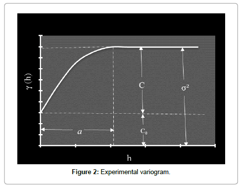
Figure 2: Experimental variogram.
Kriging
Kriging is a commonly used method of interpolation (prediction) for spatial data. The data are a set of observations of some variable(s) of interest, with some spatial correlation present. Usually, the result of kriging is the expected value and variance computed for every point within a region. Thus, it is a direct approach with a unique solution to an estimation problem and can be used to estimate the unknown value Z* of a variable at a point from the surrounding known values Zi using the following Eqn. 3.
 (3)
(3)
Where λi represent the kriging weights.
Obtaining a minimum variance of estimation  means to minimize the expression given by Eqn. 4.
 (4)
(4)
Substitution of the linear estimator can rewrite Eqn. 4 as Eqn. 5.
 (5)
(5)
To ensure no bias for the linear estimator (Eqn. 5), the constriction: should be integrated into the model. This constraint means that the local average of the observations is constant throughout the field. The minimization of a quadratic function with the presence of an equality constraint (Eqn. 6) is effected by the method of Lagrange which involves the Lagrange multiplier μ:
With the substitution of the Eqn. 6 can be rewritten as Eqn. 7.

Eqn. 7 provides ordinary kriging when cancel all the partial derivatives with respect to each λi and compared to μ. The ordinary kriging system becomes:
 (8)
(8)
The minimum estimation variance of the system (kriging variance) is determined by the substitution of kriging Eqn.s in Eqn. 8 to obtain the Eqn. 9.
 (9)
(9)
In practice, it is easier to use the matrix form of the kriging system (Eqn. 10):
 (10)
(10)
Where Ks is the (n × n) matrix of covariance between observations, ks, the (n × 1) matrix of covariance between the n observations and the point to be estimated, λ. The solution of this system is provided in matrix form as given by Eqn. 11.
 (11)
(11)
Where  (12)
(12)
And finally, (13)
(13)
Thus, Eqn. 13 is used to calculate the kriging weights λi needed to estimate a point defined by the linear estimator with Eqn. 3 [22,32].
Methodological step
To highlight the influence of the variogram model on the kriging results, we used a database made of aquifer resistivity determined in Adamawa-Cameroon region in order to investigate the productivity of local aquifers. Four different variogram models (logarithmic, Gaussian, exponential and spherical) with the same effect nugget (C0=200 Ω2m2), the same sill (σ2=5200 Ω2m2) and the same range (a=50 m) were used to interpolate the data by kriging. These variogram models are expressed by Eqns 14-17.
 (14)
(14)
 (15)
(15)
 (16)
(16)
 (17)
(17)
Correct variogram model fitting
The variogram model is chosen from a set of mathematical functions that describe spatial relationships. The appropriate model is chosen by matching the shape of the curve of the experimental variogram to the shape of the curve of the mathematical function. This is clearly illustrated in the “Golden Surfer” software we used in this study. In fact, variogram is used in the interpolative kriging technique at its second step. This step is preceded by an exploratory data analysis and a prediction [33]. During the exploratory data analysis, data were checked consistency, outliers removed and statistical distribution identified. Normal data distribution is decided when the mean and the median are very similar. However, high skewness values indicate the existence of outliers, which are very high or low measured values comparing to the dataset. The outliers are caused by a bad measurement or a bad recording, and must be transformed when they exist. During the prediction phase, four variogram models were in order to select the best-fitted one. Predictive performances of the fitted models are checked on the basis of cross validation tests. The values of mean error (ME), mean square error (MSE), root mean square error (RMSE), average standard error (ASE) and root mean square standardized error (RMSSE) are estimated to ascertain the performance of the developed models. If the predictions are unbiased, the ME should be almost nil. But because of its weaknesses due to its dependence upon the scale of the data and to its indifference to the wrongness of variogram, ME is generally standardized by the MSE, being ideally zero.
Results
Using the logarithmic model, the estimated resistivity rages between 195 and 267 Ωm. The Gaussian and spherical models produce values ranged from 100 to 480 Ωm while the exponential model provides a range of 120-420 Ωm. In general, each model produced a different result. The difference may be in the endpoints of the range or its amplitude. These differences are summarized in Table 2 and shown in Figure 3.
| Logarithmic | Exponential | Gaussian/ spherical | |
|---|---|---|---|
| Minimum | 195 | 120 | 100 |
| Maximum | 267 | 420 | 480 |
| Magnitude | 72 | 300 | 380 |
Table 2: Differences from analytical analysis between the four variogram models.
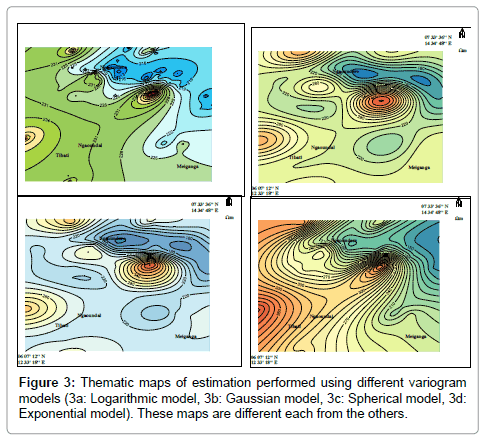
Figure 3: Thematic maps of estimation performed using different variogram models (3a: Logarithmic model, 3b: Gaussian model, 3c: Spherical model, 3d: Exponential model). These maps are different each from the others.
Discussion
In the particular case of this study, spherical and Gaussian models estimated values in the same interval (100-480 Ωm). But in general, each variogram model provides distinct result. However, despite their observed differences, all thematic maps have the same variation trend. The gradient values are constant: the minimum and maximum values are almost in the same regions respectively from one map to another. These observations are conforming to results published by many other authors worldwide. Especially, Webster and Olivier [34] several concerns related to the influence of the variogram model on the predictive investigation, and Chilès and Delfiner [31] modeled spatial uncertainty in Geostatistics. It is therefore evident that the quality and the reliability of an interpolation by kriging strongly depend on the structural analysis of field data, that is to say, the variogram model. Predictive performances of the fitted models are checked on the basis of cross validation tests. The values of mean error (ME), mean square error (MSE), root mean square error (RMSE), average standard error (ASE) and root mean square standardized error (RMSSE) are estimated to ascertain the performance of the developed models. If the predictions are unbiased, the ME should be almost nil. But because of its weaknesses due to its dependence upon the scale of the data and to its indifference to the wrongness of variogram, ME is generally standardized by the MSE, being ideally zero. However, RMSE and ASE should be calculated to indicate if the prediction errors were correctly assessed in the case where they are close. Otherwise, if the RMSE is less than the ASE (or RMSSE less than 1), then the variability of the predictions is overestimated; and if the RMSE is greater than the ASE (or RMSSE greater than 1), then the variability of the predictions is underestimated. Once the best model is selected, it is used to draw the thematic map that provides the spatial distribution of the parameter to be estimated. All these errors are expressed by Eqns (18)-(22) below [33,35].
(18)
 (19)
(19)
 (20)
(20)
 (21)
(21)
 (22)
(22)
Where σ2(xi) is the Kriging variance for location xi, Z*(xi) and Z(xi) are the estimated and the measured values of the parameter at the location xi respectively. Table 3 shows that the logarithmic model is best-fitted one. And Figure 4, we see that this is the logarithmic model that accommodates the most with the experimental variogram. This study should have many applications and impacts on environmental and earth sciences. In fact, many environmental as rainfall and earth deposits and parameters are usually called to be predicted or estimated. However, one cannot carry out measurement continuously. The parameter to be estimated is measured discretely and then, to obtain the continuous information, kriging technique is used. Nowadays, this technique based on variogram is used by so many scientists in various fields as civil protection [21], meteorology [22,30], geochemistry [13,23,26,32,33]. If authors do not take into account the paramount impact of the variogram model in such investigations, the study will be sketchy and results untruthful. This explains the importance of the present paper. Many other studies have been carried out in order to highlight the delicateness of modelling and assessment. Nshagali et al. [26] bring up the effects of scale in spatial interaction models; Patuelli and Giuseppe Arbia [36-40] published an editorial on the advances in the statistical modelling of spatial interaction data. But the present paper tackles the issue of the selection of the suitable variogram model. In fact, interpolation soft-wares automatically propose a random linear or nugget model to the user (Figure 5). When the random linear or nugget model is automatically displayed, the user should select and “add” a model that is suitable for his dataset and then fit it.
| ME | RMSE | ASE | MSE | RMSSE | |
|---|---|---|---|---|---|
| Logarithmic | 0.02 | 8.41 | 8.03 | 0.08 | 0.97 |
| Gaussian | 3.52 | 21.36 | 18.21 | 3.18 | 3.14 |
| Spherical | 5.24 | 23.21 | 20.07 | 7.01 | 3.20 |
| Exponential | 17.36 | 32.33 | 29.57 | 18.32 | 3.54 |
Table 3: Analytical characteristics of variogram models used to detect the bestfitted one.
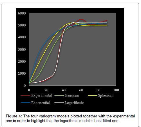
Figure 4: The four variogram models plotted together with the experimental one in order to highlight that the logarithmic model is best-fitted one.
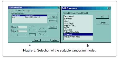
Figure 5: Selection of the suitable variogram model.
Conclusion
Many scientific studies use geographical theory and methodology to resolve environmental, social and human problems. Some of these papers deal with issues of resources assessment, prediction and management. Such investigations are generally based on the interpolative techniques such as kriging. This very important technique for especially Geoscientist and other scientists in general includes a prior step namely structural analysis based on the variogram. This step is so important that it decides on the reliability and even the veracity of the kriging results. It is therefore necessary to well apply during the cross validation test in order to select the best-fitted variogram model before predictive analysis. In fact, the selection of a variogram model can be explicit or implicit (incorporated in software). This article illustrates how the use of an inappropriate variogram model can seriously distort the results of an evaluation or assessment or prediction survey.
References
- Cheng T, Haworth J, Wang J (2012) Spatio-temporal autocorrelation of road network data. J Geographical Systems 14: 389-413.
- Gerkman L (2012) Empirical spatial econometric modelling of small scale neighbourhood. J Geographical Systems 14: 283-298.
- O’Kelly ME, Niedzielski MA, Gleeson J (2012) Spatial interaction models from Irish commuting data: variations in trip length by occupation and gender. J Geographical Systems 14: 357-387.
- Yates J, Sanjeevi S (2012) Assessing the impact of vulnerability modeling in the protection of critical infrastructure. J Geographical Systems 14: 415-435.
- Singleton AD, Wilson AG, O’Brien O (2012) Geodemographics and spatial interaction: an integrated model for higher education. J Geographical Systems 14: 223-241.
- LeSage JP, Llano C (2013) A spatial interaction model with spatially structured origin and destination effects. J Geographical Systems 15: 265-289.
- Nazneen FC (2013) A spatial panel ordered-response model with application to the analysis of urban land-use development intensity patterns. J Geographical Systems 15: 1-29.
- Bourgault G (2014) Revisiting Multi-Gaussian Kriging with the Nataf Transformation or the Bayes’ Rule for the Estimation of Spatial Distributions. Math Geosci 46: 841-868
- Kolyukhin D,Tveranger J (2014) Statistical Analysis of Fracture-Length Distribution Sampled Under the Truncation and Censoring Effects. Math Geosci 46: 733-746
- LeSage JP, Sheng Y (2014) A spatial econometric panel data examination of endogenous versus exogenous interaction in Chinese province-level patenting. J Geographical Systems 16: 233-262.
- Mack EA, Zhang Y, Rey S, Maciejewski R (2014) Spatio-temporal analysis of industrial composition with IVIID: an interactive visual analytics interface for industrial diversity. J Geographical Systems 16: 183-209.
- Sun XL, Wu YJ,Wang HL,Zhao YG, Zhang GL (2014) Mapping Soil Particle Size Fractions Using Compositional Kriging, Cokriging and Additive Log-ratio Cokriging in Two Case Studies Math Geosci 46: 429-443.
- Arétouyap Z, Nouayou R, Njandjock NP, Asfahani J (2015) Aquifers productivity in the Pan-African context. Earth SystSci 124: 527-539.
- Chaney RA, Rojas GL (2015) Spatial patterns of adolescent drug use. Applied Geography 56: 71-82.
- Eidsvik J (2015) Pyrcz and Deutsch: Geostatistical Reservoir Modeling. Math Geosci 47:497-499.
- Keumseok K, Grady SC, Vojnovic I (2015) Using simulated data to investigate the spatial patterns of obesity prevalence at the census tract level in metropolitan Detroit. Applied Geography 62: 19-28.
- Melnikova Y, Zunino A, Lange L,Cordua KS, Mosegaard K (2015) History Matching Through a Smooth Formulation of Multiple-Point Statistics. Math Geosci 47:397-416
- Mishra NB, Chaudhuri G (2015) Spatio-temporal analysis of trends in seasonal vegetation productivity across Uttarakhand, Indian Himalayas, 2000-2014. Applied Geography 56: 29-41.
- Zunkel P (2015) The spatial extent and coverage of tornado sirens in San Marcos. Texas Applied Geography: 308-312.
- Sacks J, Schiller S (1988) Spatial designs. In Statistical Decision Theory and Related Topics IV, Gupta SS, Berger JO (eds). Springer-Verlag: New York: 385-399.
- Zamani A, Mirabadi A (2011) Optimization of sensor orientation in railway wheel detector, using kriging method. Journal of Electromagnetic Analysis and Applications 3: 529-536.
- Arétouyap Z, Njandjock NP, Bisso D, Nouayou R, Lengué B, et al. (2014a) Investigation of groundwater quality control in Adamawa-Cameroon region. J Applied Sci 14: 2219-2233.
- Arétouyap, Z, Njandjock NP, Ekoro NH, Méli’i JL, Lepatio TSA (2014b) Investigation of groundwater quality control in Adamawa-Cameroon region. J Applied Sci 14: 2309-2319.
- Chevalier C, Ginsbourger D, Bect J, Vazquez E, Picheny V, Richet Y (2014) Fast parallel kriging-based stepwise uncertainty reduction with application to the identification of an excursion set. Technometrics 56: 455-465.
- Hamel P, Sambou DC, Darces M, Beniguel Y, Hélier M (2014) Kriging method to perform scintillation maps based on measurement and GISM model. Radio Science 49: 746-752.
- Nshagali BG, Njandjock NP, Meli’i JL, Arétouyap Z, Manguelle-Dicoum E (2015) High iron concentration and pH change detected using statistics and geostatistics in crystalline basement equatorial region. Environ Earth Sci 73: 7135-7145.
- ToteuSF,Ngako V,AffatonP,Nnange JM, Njanko TH(2000)Pan-African tectonic evolution in Central and Southern Cameroon: Tranpression and transtension during sinistral shear movements. J Afr Earth Sci 36: 207-214.
- Segalen P (1967) Soils and geomorphology of Cameroon. Cahier ORSTOM-SériePédologie 5: 137-187.
- Toteu SF, Penaye J, Poudjom DY (2004) Geodynamic evolution of the Pan-African belt in central Africa with special reference to Cameroon. Can J Earth Sci 41: 73-85.
- Caridad RP, Jury MR (2013) Spatial and temporal analysis of climate change in Hispañola. TheorApplClimatol 113: 213-224.
- Chilès JP, Delfiner P (2012) Geostatistics: Modeling Spatial Uncertainty, 2nd edition. John Wiley and Sons Inc: New York.
- Meli’i JL, Bisso D, Njandjock NP, Ndougsa T, Mbanga AF, et al. (2013) Water table control using ordinary kriging in the southern part of Cameroon. J Applied Sci 13: 393-400.
- Gorai AK, Kumar S (2013) Spatial distribution analysis of groundwater quality index using GIS: A case study of Ranchi municipal corporation (RMC) area. Geoinfor. Geostat: An Overview.
- Webster R, Oliver MA (2007) Geostatistics for Environmental Scientists, 2nd edition. John Wiley & Sons: Chichester.
- Goovaerts P (1997) Geostatistics for natural resources evaluation. Oxford University Press, Applied Geostatistics Series: London.
- Patuelli R, Giuseppe A (2013) Editorial: Advances in the statistical modelling of spatial interaction data. J Geographical Systems 15: 229-231.
- Binita KC, Marshall, SJ, Gaither CJ (2015) Climate change vulnerability assessment in Georgia. Applied Geography 62: 62-74.
- Diodato N, Esposito L, Bellocchi G, Vernacchia L, Fiorillo F, et al. (2013) Assessment of the spatial uncertainty of nitrates in the aquifers of the Campania plain (Italy). Am J Climate Change 2: 128-137.
- Giuseppe A, Petrarca F (2013) Effects of scale in spatial interaction models. Journal of Geographical Systems 15: 249-264.
- Maréchal A (1976) Geology and geochemistry of mineral thermal resources of Cameroon. Doc ORSTOM 59: 169-176.
Citation: Arétouyap Z, Nouck NP, Nouayou R, Méli’i JL, Kemgang Ghomsi FE, et al. (2015) Influence of the Variogram Model on an Interpolative Survey Using Kriging Technique. J Earth Sci Clim Change. 6: 316. Doi: 10.4172/2157-7617.1000316
Copyright: © 2015 Arétouyap Z, et al. This is an open-access article distributed under the terms of the Creative Commons Attribution License, which permits unrestricted use, distribution, and reproduction in any medium, provided the original author and source are credited.
Share This Article
Open Access Journals
Article Tools
Article Usage
- Total views: 11674
- [From(publication date): 12-2015 - Apr 19, 2024]
- Breakdown by view type
- HTML page views: 10963
- PDF downloads: 711