


Abstract
The Coronal Global Evolutionary Model (CGEM) provides data-driven simulations of the magnetic field in the solar corona to better understand the build-up of magnetic energy that leads to eruptive events. The CGEM project has developed six capabilities. CGEM modules (1) prepare time series of full-disk vector magnetic field observations to (2) derive the changing electric field in the solar photosphere over active-region scales. This local electric field is (3) incorporated into a surface flux transport model that reconstructs a global electric field that evolves magnetic flux in a consistent way. These electric fields drive a (4) 3D spherical magnetofrictional (SMF) model, either at high resolution over a restricted range of solid angles or at lower resolution over a global domain to determine the magnetic field and current density in the low corona. An SMF-generated initial field above an active region and the evolving electric field at the photosphere are used to drive (5) detailed magnetohydrodynamic (MHD) simulations of active regions in the low corona. SMF or MHD solutions are then used to compute emissivity proxies that can be compared with coronal observations. Finally, a lower-resolution SMF magnetic field is used to initialize (6) a global MHD model that is driven by an SMF electric field time series to simulate the outer corona and heliosphere, ultimately connecting Sun to Earth. As a demonstration, this report features results of CGEM applied to observations of the evolution of NOAA Active Region 11158 in 2011 February.
Export citation and abstract BibTeX RIS
1. Introduction to the Coronal Global Evolutionary Model
The existence of full-disk high-resolution vector magnetic field data taken with an uninterrupted cadence of several minutes from instruments such as the Helioseismic and Magnetic Imager (HMI; Scherrer et al. 2012; Schou et al. 2012; Hoeksema et al. 2014) on NASA's Solar Dynamics Observatory (SDO; Pesnell et al. 2012) motivates us to ask these questions: is it possible to use these data to construct a physics-based model for the evolution of the magnetic field in the Sun's atmosphere? Can such a data-driven model provide useful insight and predictive capability for understanding how magnetic energy builds up in the solar corona before the occurrence of solar flares and coronal mass ejections? The overall goal of the Coronal Global Evolutionary Model (CGEM) is to provide such a data-driven modeling capability. This report describes the scope and capabilities of CGEM, a project funded by Strategic Capability grants from NASA's Living With a Star Program and from the National Science Foundation (Fisher et al. 2015; see also http://cgem.ssl.berkeley.edu). To illustrate CGEM's capabilities, this article focuses on using data and simulations of the evolution of NOAA Active Region (AR) 11158 to demonstrate the different components of CGEM, show how they are related to one another, and illustrate at a practical level what is involved in using the various component models of CGEM.
A principal objective of CGEM is to develop a spherical version of the magnetofrictional model (Cheung & DeRosa 2012) of the solar corona to study the build-up of magnetic energy. The spherical magnetofrictional model (SMF) is driven by time series of magnetic and electric fields determined at the solar photosphere from measurements of the photospheric magnetic and velocity fields made by the HMI instrument on NASA's SDO mission. The SMF can be run on either active-region scales or on global scales. Output from the SMF model can then be used as a starting point for more detailed MHD simulations.
The CGEM project comprises four main science activities:
- 1.Implement enhanced processing of SDO/HMI vector and full-disk line-of-sight magnetogram sequences and HMI Doppler velocity measurements and make these available to the solar physics and space-weather communities.
- 2.Use these data to compute electric fields at the photosphere, on both active-region and global scales, and make the electric field solutions publicly available.
- 3.Use the time sequence of photospheric magnetic field and electric field maps to drive a time-dependent, nonpotential model based on magnetofriction for the magnetic field in the coronal volume, both in active regions and globally. This is done in spherical geometry, in either spherical wedge configurations for active regions or for the global Sun. Hereafter, the term "spherical wedge" refers to a finite subvolume in spherical coordinates, defined by upper and lower limits of radius, latitude, and longitude.
- 4.For unstable configurations discovered with the SMF model, perform follow-up studies using MHD models to provide more realistic dynamics for erupting magnetic structures.
The detailed workflow to accomplish these activities is a series of linked tasks, described below.
- 1.The first task is to perform enhanced HMI data processing (EHDP) on the input measurements needed to compute electric fields at the solar photosphere.
- 2.
- 3.The local electric field patches are inserted into a global surface flux transport (SFT) model that allows magnetic flux to emerge consistently with the model evolution computed outside of active regions.
- 4.The electric field in CGEM patches can be used to run the SMF model at active-region scales, or the output of the SFT model can be used as input for the global version of the SMF model.
- 5.The local SMF model output can be used as a starting point for local-scale radiative MHD (RADMHD) simulations.
- 6.To help visualize the state of the corona from SMF or RADMHD simulations, an emissivity model, based on the square of the current density, can be used to construct a projected proxy coronal image (J2EMIS).
- 7.The global version of the SMF model can be used to provide input for global coronal-heliospheric MHD (GHM) simulations that extend into the heliosphere.
The order of topics discussed in this paper follows the workflow requirements. To clarify the relationship of the tasks in an intuitive fashion, we illustrate the workflow order in Figures 1 and 2.

Figure 1. Workflow diagram showing how the EHDP task generates enhanced data products (corrected HMI vector magnetograms, calibrated Doppler maps, and local correlation-tracking velocities) that feed the PDFI task (electric field inversion software) to produce a time series of photospheric electric field maps. The quantity  is the photospheric vector magnetic field,
  is the observed Doppler velocity, and
  is the derived horizontal velocity at the photosphere.
Download figure:
Standard image High-resolution image
Figure 2. Local electric field maps can be used to drive the local spherical magnetofrictional (SMF) model above active regions, or they can be ingested into the global surface flux transport (SFT) model that produces quantities used to drive the global SMF model. The output from SMF models can then be used as the starting point for MHD simulations in active regions (RADMHD), or a global heliospheric MHD (GHM) model.
Download figure:
Standard image High-resolution imageThe remainder of the paper is outlined below.
First, in Section 2, the analysis of the HMI data for NOAA AR 11158 is described (EHDP). This is followed by a discussion of the calculation of the electric field solutions at the photosphere (PDFI). The data analysis and electric field calculations in general are described in full detail in Fisher et al. (2020), so the emphasis here is on how the results can be obtained from the Joint Science Operations Center (JSOC) site to be used as input into the other elements of the CGEM model.
The CGEM SFT model is described in Section 3. A novel aspect of this particular flux transport model is that it is electric field based, allowing us to more easily interface the model's electric field solutions with those from the smaller-scale active region solutions described in Section 2. Examples showing the global magnetic field configuration during the two months leading up to the CME eruption of 2011 February 12 using the SFT model are shown.
In Section 4, the SMF model is discussed. Considerable development effort has been completed since the model's initial description in Cheung & DeRosa (2012), and the most important of these changes are described. A simulation of NOAA AR 11158 is performed to both demonstrate the usage of the model and to show some of the resulting output magnetic configurations. The current status of the model at NASA's Community Coordinated Modeling Center (CCMC) is summarized.
In Section 5 we present the implementation of three-component data driving for AR-scale MHD simulations (RADMHD), using initial states from the SMF model and electric field solutions at the photosphere.
Section 6 describes how the current-based emissivity model (J2EMIS) initially described by Cheung & DeRosa (2012) has been modified to visualize magnetic field configurations in global spherical geometries. Both the advantages and limitations of this software are discussed, along with some examples of the AR 11158 magnetic configuration shown in a global context.
We discuss the coupling of the global version of the SMF model to our global coronal-heliospheric MHD model (GHM) in Section 7, using the two months prior to 2011 February 12 to illustrate the coupling of the two models and the global magnetic field evolution.
Finally, in Section 8, we summarize the work presented here, then discuss the role of CGEM models in understanding fundamental problems in heliophysics, and suggest directions for future work employing the CGEM models and concepts used in the development of these models.
2. Enhanced HMI Data Processing to Estimate the Photospheric Electric Field
This section presents an overview of the enhanced processing of HMI magnetic and velocity data, the electric field inversion software (called PDFI_SS), and ways to access related data products through the SDO JSOC. For a detailed description of these steps, please consult Sections 2–4 of Fisher et al. (2020). Figure 3 shows an example of the output data.
Figure 3. A snapshot of the processed HMI data for AR 11158. The top and middle rows show the vector magnetic and velocity fields. They are the average of the two input frames at 2011.02.15_00:00:00_TAI and 00:12:00_TAI. The lower row shows the inferred electric field at 00:06:00_TAI. Only the central portion of the frame is shown; the weaker field and the padding are excluded. The Doppler velocity plotted here is scaled by 0.1 with blueshift ( ) as positive. The original values in the JSOC data set range between
  with redshift (
 ) as positive. For more details, see Section 2. An animation of the entire 6.4 day data set every 12 minutes from 2011.02.10_14:18:00_TAI to 2011.02.16_23:42:00_TAI is available.
(An animation of this figure is available.)
Download figure:
Video Standard image High-resolution imageIn order to derive electric fields with the PDFI_SS software, we must first process the full-disk HMI data into a form compatible with PDFI_SS. Five steps are required to get the data into a suitable form: (1) estimate and remove the Doppler velocity "convective blueshift" bias, due to the overweighting of the hot, upflowing plasma as compared to the cooler, downflowing plasma in the spectral line intensity profile (Welsch et al. 2013); (2) isolate and track the data centered on an AR of interest with a rotation rate defined by the AR center, and map the data into a corotating reference frame; (3) correct short-lived azimuth fluctuations in transverse magnetic fields, and then map the resulting magnetic field, Doppler, and line-of-sight unit-vector data into a Plate Carrée grid; (4) apply the Fourier Local Correlation Tracking (FLCT) algorithm to successive radial field magnetograms to estimate the apparent horizontal motions; and finally, (5) add a ribbon of zero-value data around each of the data arrays. We find that this "zero padding" improves the quality of the electric field inversions. As a result of (1)–(5), we derive a final set of vector magnetic and non-orthogonal velocity field components, (Bx , By , Bz ) and (vx , vy , vl ) (see Figure 3). In this section of this article, the subscripts x, y, and z denote the longitudinal, latitudinal, and radial components of our vectors, respectively. The subscript l denotes the component of a vector projected onto the observer's line of sight, with away from the observer (redshift) positive. The source code that performs this calculation is available. 9
We then use PDFI_SS software to derive the electric field vector,  , in the solar photosphere from a time sequence of masked input vector magnetogram and velocity data described above (the "PDFI" task). We construct masks to exclude areas where we expect the noise in the HMI magnetic field to produce unreliable electric fields (
 G). This threshold value is considerably greater than the estimated uncertainty in the magnetic field components, but it is important to remember that the most important PDFI input quantity is the temporal difference in the magnetic field at two successive time steps, not the magnetic field at a given time. The choice of the threshold value is a compromise between good signal-to-noise ratio in the computed temporal derivative, and the desire to analyze as much of the data in the images as possible. Empirical studies we have done suggest an appropriate threshold is in the range of 200–300 G. Here, we adopt 250 G. Lumme et al. (2019) adopted 300 G. The PDFI_SS software (Fisher et al. 2020) is based on the PDFI technique for deriving electric fields (Kazachenko et al. 2014). The letters in PDFI stand for poloidal-toroidal decomposition (PTD), Doppler, FLCT, and Ideal, reflecting different contributions into the total electric field as described below. The main idea of the PDFI method is that the electric field can be derived from the observed magnetic field components by uncurling Faraday's law. While any such inversion is non-unique, due to contributions from gradients of scalar functions that have zero curl, in PDFI we make use of additional information. This includes Doppler shifts near polarity inversion lines, flow fields from FLCT, and other constraints, which allow us to compute the electric fields from scalar potentials that can then be added to the solution of Faraday's law to find the total electric field.
Figure 3 shows an example of the processed data described above: the three components of the magnetic field (Bx , By , Bz ), horizontal and Doppler velocities (vx , vy , vl ), and electric field (Ex , Ey , Ez ), in the central part of AR 11158. The animation 10 shows the evolution of these variables over 6.4 days. The movie shows several interesting phenomena of AR dynamics previously described in Kazachenko et al. (2015) and Lumme et al. (2019). The movie also exhibits "flickering" of the electric fields (Ex , Ey , Ez ) in the surrounding quiet-Sun regions caused by the sensitivity of the PDFI method to noise in the magnetic field and velocity data. We estimate this effect to lead to a ∼1% error in the overall energy and helicity budgets of the AR (see Section 4.2 of Lumme et al. 2019). Time series made with higher-cadence HMI data (90 s or 120 s) have a lower signal-to-noise ratio than the 12 minute data and show much larger amplitude flickering.
The PDFI approach has been extensively tested using synthetic data—magnetograms extracted from MHD simulations where the true photospheric electric field is known (Kazachenko et al. 2014). Using anelastic pseudo-spectral ANMHD simulations of an emerging magnetic bipole in a convecting box (Abbett et al. 2000, 2004), we have shown that the PDFI method significantly improves recovery of the simulation's electric field and energy fluxes when compared to the original PTD method of Fisher et al. (2010; see Table 3 of Kazachenko et al. 2014). The PDFI inversions compare favorably to or tend to be more accurate than certain other state-of-the-art velocity inversion methods (e.g., DAVE4VM; see Table 4 in Kazachenko et al. 2014 and Figures 11 and 12 in Schuck 2008). Recently, we have improved the accuracy of the PDFI numerical method, replacing the original PDFI "Cartesian centered" (CC) grid with a more accurate "PDFI_SS" version discretized on a "spherical staggered" (SS) grid (Fisher et al. 2020). PDFI_SS software (Fisher et al. 2020) is written as a general purpose FORTRAN library and can be easily linked to other FORTRAN, C/C++, or Python programs. For routine CGEM processing, the SDO/HMI JSOC pipeline software calls one of the high-level Fortran subroutines within PDFI_SS to compute AR electric fields.
The processed HMI input data sets and the output data sets from PDFI_SS are publicly available through the SDO JSOC website, 11 with series names cgem.pdfi_input and cgem.pdfi_output, respectively. SDO data analysis manuals contain the details on data query and retrieval methods. 12 , 13 Each JSOC record in the two data series is identified via two keywords, CGEMNUM and T_REC. The keyword CGEMNUM is the NOAA AR number when the CGEM region corresponds to a single named AR and is equal to 100,000 plus the HMI SHARP number when it does not. The keyword T_REC corresponds to the observation time and differs slightly between cgem.pdfi_input and cgem.pdfi_output. The nominal T_REC is designated at 06, 18, 30, 42, and 54 minutes after the hour for cgem.pdfi_output, and at 00, 12, 24, 36 and 48 minutes after the hour for cgem.pdfi_input. For example, users can find a pair of input records for AR 11158 at the beginning of 2011 February 15 with cgem.pdfi_input[11158][2011.02.15_00:00-2011.02.15_00:12], which includes the vector magnetic field, FLCT velocity field, Doppler velocity, and local unit normal vectors. The corresponding PDFI output can be found with cgem.pdfi_output[11158] [2011.02.15_00:06], containing vector magnetic fields, electric fields, the Poynting flux, and the helicity injection rate contribution function on a staggered grid (for a full list of output variables, see Section 10.3 of Fisher et al. 2020). Regarding the computed helicity injection rate, see the comments following Equation (30) in Fisher et al. (2020).
To provide a sense for the computational resources needed to produce electric field solutions, our tests show that using a single processor on a 2016 model Macbook Pro laptop, electric field solutions at a single time are produced in roughly 5 s given vector magnetogram and Doppler data for the two consecutive time steps of the input data series for AR 11158.
Finally, we wish to point out another data product developed as part of CGEM to understand magnetic activity. The JSOC data series cgem.lorentz provides a comprehensive calculation of Lorentz forces in all of the active regions observed by HMI (Sun 2014). For each SHARP region at each time stamp, this data series provides three maps of the photospheric Maxwell stress tensor and their surface integral. The latter can be viewed as a proxy for the integrated Lorentz force in the entire volume above the photosphere; it is computed using the divergence theorem and a few simplifying assumptions (see, e.g., Fisher et al. 2012). During eruptive solar events, Lorentz forces computed with HMI are sometimes observed to undergo abrupt changes that coincide in time with the events. Fast evolution of the photospheric field during major solar eruptions is also clear (Sun et al. 2017). The data series can also be useful for evaluating the "force-freeness" of the photospheric field when it is used as the input for coronal field extrapolation (Wiegelmann & Sakurai 2012; Duan et al. 2020).
3. A Global Surface Flux Transport Model Based on the Electric Field
Global SFT models describe the evolution of the magnetic field Br on the photosphere of the Sun. SFT models are found to match the observed evolution of the radial component Br of the photospheric magnetic flux on the Sun reasonably well and are widely used within the field of solar physics (for additional details, see the review by Jiang et al. 2014). At their core, these models solve the radial component of the magnetic induction equation,

on a spherical surface using prescriptions for the advection of magnetic flux (via the  term) and the dispersal of flux (via the diffusion term) across the photosphere. These flow patterns are often characterized by the empirically determined advection velocity
  and the diffusion coefficient η. New flux is added to an SFT model either via a source function or by assimilating (or directly inserting) observed magnetic field measurements into the model.
In this section, we describe a different implementation of a global SFT model based on photospheric electric fields. Here, the evolution of Br is governed by the radial component of Faraday's Law,

which describes the evolution of Br on a spherical surface in terms of the curl of horizontal (i.e., zonal and meridional) electric fields. The factor c is the speed of light (cgs units are used throughout this section).
The PDFI method for processing the HMI Doppler and vector magnetogram data for active regions described in Section 2 results in time series of photospheric electric field data within and around active regions covered by CGEM Patches. This series of photospheric electric fields is, by design, consistent with the observed evolution of surface magnetic flux within each CGEM Patch. To capture the life cycles of observed active regions on larger scales, including the subsequent dispersal of flux into surrounding quiet-Sun regions, the CGEM SFT model incorporates such time series of electric field data into a global model for the horizontal electric field  that describes the evolution of the photospheric radial magnetic field over the entire photosphere.
To obtain a global map of  , the electric field for locations outside of CGEM Patches is required. By adapting the same concepts used in more traditional SFT models, combining Equations (1) and (2) indicates that the evolution of Br
is governed by
, the electric field for locations outside of CGEM Patches is required. By adapting the same concepts used in more traditional SFT models, combining Equations (1) and (2) indicates that the evolution of Br
is governed by

where  represents the empirically determined horizontal flow fields (i.e., differential rotation and meridional flows), ηh
is a horizontal diffusion coefficient, and
represents the empirically determined horizontal flow fields (i.e., differential rotation and meridional flows), ηh
is a horizontal diffusion coefficient, and  is the unit vector in the radial direction. The CGEM SFT model uses a differential rotation velocity
  of the form

where θ is the heliographic colatitude and  is the unit vector in the longitudinal direction. The quantities (A, B, C) are set to (2.865, −0.405, −0.422) × 10−6 rad s−1 as found by Komm et al. (1993a), who determined these values by cross-correlating magnetograms on successive days over a time interval of more than 15 yr. A companion study by Komm et al. (1993b) determined a meridional flow pattern
  having the functional form

where  is the unit vector in the colatitudinal direction and
  m s−1. Taking the curl of
  from Equation (3), using a
  equal to
  , and choosing
  to be 300 km2 s−1, gives
  for the CGEM SFT model by Equation (2). A snapshot from the global SFT model is shown in Figure 4.

Figure 4. Maps of Br
(left panel) and  (right panel) from the CGEM SFT model for 2011 February 14 at 08:21 UT. PDFI electric fields associated with ARs 11140–11166 from the first two months of 2011 were inserted in the
  maps, from which the evolution of Br
was determined. The rectangular boundary of the CGEM Patch associated with AR 11158 is outlined in a dashed line. The maps use a Mollweide projection with grid lines spaced every 60° and is centered on Carrington longitude 60°.
maps, from which the evolution of Br
was determined. The rectangular boundary of the CGEM Patch associated with AR 11158 is outlined in a dashed line. The maps use a Mollweide projection with grid lines spaced every 60° and is centered on Carrington longitude 60°.
Download figure:
Standard image High-resolution imageThe use of time series of  to drive the evolution of Br
confers several advantages.
to drive the evolution of Br
confers several advantages.
First, knowing  enables the evaluation of the Poynting flux
  through the photospheric surface to be quantified in the model, because
  . In the PDFI scheme described above, the use of both the observed vector magnetic field and the velocity field in constraining
  within CGEM Patches also allows
  to be constrained within the CGEM Patches, allowing the energetics of the flux-emergence process to be studied more readily.
Second, it is more straightforward to use time series of  (compared with time series of
  ) as a time-evolving lower boundary condition for data-driven models of the overlying coronal dynamics. One such data-driven model is described in the next section.
Third, by using  , the net flux of Br
through the model is always preserved, regardless of the flux (im)balance within each CGEM Patch.
14
In contrast, more traditional SFT models often suffer from flux-imbalance issues, which may be significant when, for example, active regions are not fully contained within the assimilation window. One common strategy to deal with such flux-imbalance issues is to subtract off the net imbalance over the whole spherical surface in the model, a treatment that necessarily affects the global distribution of flux in these models and may cause far-removed neutral lines and other features of interest to shift. In the electric-field-based scheme presented here, any flux imbalance within a CGEM Patch ends up being balanced by an offsetting amount of flux distributed uniformly within the patch, resulting in the compensatory flux being local to the CGEM Patch.
, the net flux of Br
through the model is always preserved, regardless of the flux (im)balance within each CGEM Patch.
14
In contrast, more traditional SFT models often suffer from flux-imbalance issues, which may be significant when, for example, active regions are not fully contained within the assimilation window. One common strategy to deal with such flux-imbalance issues is to subtract off the net imbalance over the whole spherical surface in the model, a treatment that necessarily affects the global distribution of flux in these models and may cause far-removed neutral lines and other features of interest to shift. In the electric-field-based scheme presented here, any flux imbalance within a CGEM Patch ends up being balanced by an offsetting amount of flux distributed uniformly within the patch, resulting in the compensatory flux being local to the CGEM Patch.
Numerically, the CGEM SFT model is computed on a spherically staggered grid analogous to the grid used in the PDFI electric field determinations of Section 2. The only differences are that the grid spans the full spherical surface instead of a localized CGEM Patch and that the SFT model has lower resolution by a factor of at least 10 in order to be computationally feasible. Using a staggered grid is ideally suited for taking accurate curls of  and additionally enables accurate and fast downsampling to occur as long as the downsampling factor is an integral divisor of the original grid dimensions (see Figure 8 of Fisher et al. 2020). The staggered-grid scheme used here for the purpose of calculating curls is an example of the constrained-transport method, which we believe was first used in an astrophysical setting by Evans & Hawley (1988). Here, we also use the upwind slope-limiting scheme described in Equation (48) of Stone & Norman (1992), which follows the method developed in van Leer (1977).
One issue that arises when inserting the localized PDFI electric fields into a global  map is that of a mismatch at the interface between the two electric field domains. While the curls of these electric fields respectively yield the desired evolution of Br
both within and outside of each CGEM Patch, taking the curl across the interface can yield spurious values of
map is that of a mismatch at the interface between the two electric field domains. While the curls of these electric fields respectively yield the desired evolution of Br
both within and outside of each CGEM Patch, taking the curl across the interface can yield spurious values of  . This mismatch results because the two types of
  maps may differ by the gradient of an unknown scalar function and still yield the proper
  within each respective domain; however, there is no guarantee that these will match across the perimeter of the CGEM Patch. To address this issue, before inserting a PDFI electric field map into the global map of
  , we add to the PDFI electric field map a curl-free
  , calculated such that the values of
  of these curl-free fields around the perimeter of the CGEM Patch match the external values determined from the global
  map corresponding to the large-scale flows. This treatment eliminates the mismatch of electric fields around the perimeters of the CGEM Patches without affecting the evolution of Br
. For additional details, we refer the reader to Section 5.1 of Fisher et al. (2020) in which this process is described more fully.
map corresponding to the large-scale flows. This treatment eliminates the mismatch of electric fields around the perimeters of the CGEM Patches without affecting the evolution of Br
. For additional details, we refer the reader to Section 5.1 of Fisher et al. (2020) in which this process is described more fully.
Another issue that materializes when inserting PDFI electric fields into a global  map is that the PDFI electric fields only capture the evolution of active regions at times when they are observed. As a result, any evolution that occurs when the region of interest is not on the Earth-facing side of the Sun, or when data are missing (for example, in short daily intervals during the SDO spacecraft's semiannual eclipse seasons) is not represented. During such intervals, the "nudging" scheme described in Section 5.2 of Fisher et al. (2020) provides a way to infer a valid
  that affects a smooth transition between the Br
at one point in time to the Br
at a later time. The nudging scheme is used both to bridge data dropouts and to (roughly) approximate the emergence of flux that occurs prior to the active-region flux within a CGEM Patch appearing on the east limb.
that affects a smooth transition between the Br
at one point in time to the Br
at a later time. The nudging scheme is used both to bridge data dropouts and to (roughly) approximate the emergence of flux that occurs prior to the active-region flux within a CGEM Patch appearing on the east limb.
Global maps of  computed for two separate weeks-long intervals are available in JSOC data series cgem.sft_global_nlong0300_noncontiguous, cgem.sft_global_nlong0600_noncontiguous, and cgem.sft_global_nlong1200_noncontiguous. These data series contain global
  maps at different spatial resolutions, in which the number of grid points spanning the full 360° of longitude is 300, 600, and 1200 pixels, respectively. The time intervals for which global
  data are available include 2011 January and February (containing regions such as AR 11158) as well as the end of 2014 March (containing regions such as AR 12017). Assuming data from the cgem.pdfi_output data series are immediately accessible, advancing the global SFT model by one day in time takes approximately 1, 10, or 100 minutes of wall-clock time on a desktop workstation, depending on spatial resolution.
4. A Data-driven Spherical Magnetofrictional Model for Coronal Energy and Helicity
The SMF model is an adaptation of the Cartesian MF code (Cheung & DeRosa 2012; Cheung et al. 2015). It advances Faraday's induction equation,

where  is the vector potential and
  is the electric field. Toriumi et al. (2020) performed tests of a number of data-driven models (MF and MHD) against a ground-truth MHD model of flux emergence and found the
  -field-driven MF model to quantitatively reproduce the magnetic field energy and relative helicity in the corona.
The CGEM SMF code solves the induction equation on a spherical coordinate system consisting of computational cells defined on an  grid, where r is the radial distance from the solar center and ϕ and θ are the longitudinal and latitudinal coordinates, respectively. Like the original Cartesian version, the code uses a staggered grid such that
- 1.the vector potential
 , the electric field , and the current density are defined on cell edges,
 - 2.the magnetic field is defined on cell faces, and
- 3.the MF velocity is defined at cell corners.


The magnetofrictional coefficient is  , where
  km2 s−1. Cheung & DeRosa (2012) chose a height-dependent profile for
  such that the coefficient tapered to zero at the photosphere, motivated by comments regarding the nature of MF evolution by Low (2010). The latter point out that under a line-tied scenario (i.e.,
  at
at  ) in which the photospheric radial flux distribution does not change, MF evolution will create tangential discontinuities, leading to magnetic reconnection near the photospheric boundary which violates line tying. In a data-driven model, the aim is to continuously drive the bottom boundary based on the observed evolution (i.e., not line tying) regardless of how the model coronal field behaves. As shown in Figure 7 of Toriumi et al. (2020), the model coronal MF is never entirely force free (neither is the benchmark MHD model in that study), and it is the residual forces that drive the coronal field to evolve. Because the MF velocity is never used at the bottom boundary, there is no need to taper
  to zero. The SMF model is driven at the bottom boundary by setting
  and
and  , which is supplied by either PDFI inversions (Section 2) or the CGEM SFT model (Section 3).
Figure 5 shows the radial component of the magnetic field (Br
) at different heights  in the SMF coronal field model of AR 11158. The evolution of the coronal field was driven by CGEM PDFI electric field inversions spanning the 6.4 day time interval 2011-02-10T14:18:00 to 2011-02-16T23:42:00. To prepare an initial condition for
  in the computational volume,
  was set to zero for
  . In this state, there is a mismatch between the HMI-measured
  and the model field. We use the "nudging" technique described in Section 5.2 of Fisher et al. (2020) to solve for a correction to the transverse components of the vector potential
  at
at  ), such that
  at
at  . The nudging is essentially the same as subroutine enudge_ll described in that article, but with the source code incorporated into the SMF model directly, rather than by linking to the PDFI_SS library.
  in the computational volume is then iteratively updated by advancing Equation (6) with the MF method. This relaxation method results in a coronal field that is matched to the initial photospheric flux distribution at 2011-02-10T14:18:00.

Figure 5. Synthetic magnetograms (Br ) from the CGEM Spherical Magnetofrictional (SMF) model of AR 11158. Columns are different times. Blue and red denote positive and negative values of Br ; color bars in each row show scale at each height. Note that the color maps are saturated, i.e., the color map range shown is smaller than the actual range of magnetic field values.
Download figure:
Standard image High-resolution imageFor the evolving SMF run, the transverse components of the electric field are set by electric field solutions from the PDFI inversion (available via the JSOC data series cgem.pdfi_output). By construction, the PDFI electric fields are consistent with the observed evolution of  as measured by HMI. Imposing this set of electric fields at the bottom boundary of the SMF model drives the evolution of the coronal field in response to the observed photospheric evolution. The top and side boundary conditions are implemented such that the field crossing the boundaries is normal to the surface, and the MF-computed velocity field is extrapolated out (with zero gradient) into the ghost cells. Using a Cartesian version of the MF model to simulate AR 11158, Chintzoglou et al. (2019) showed that the E-field-driven coronal field generated a twisted flux rope hours prior to the time of the observed X2 flare at 2011-02-15T01:43:00. The production of a twisted flux rope also occurs in the spherical MF model.
The complete 6.4 day computational run at the original spatial sampling of the PDFI electric field (as described in this section) required approximately 200,000 CPU hours. The SMF module has been delivered to NASA's CCMC and is being implemented for use by researchers.
5. A Data-driven Active-region-scale Radiative MHD Model
5.1. Physics of the Model
Abbett (2007) developed RADMHD, one of the first numerical models capable of evolving magnetic fields over the vast range of physical conditions and the disparate spatial and temporal scales characteristic of the convection-zone-to-corona system. Since its initial description in that article, RADMHD has undergone significant updates to improve its ability to model active region evolution in a global environment (Abbett & Fisher 2012; Abbett & Bercik 2014). RADMHD now has the option to evolve the following MHD system of conservation equations on a Cartesian or a spherical-polar block non-uniform mesh, either globally or over a subset of solid angles:


Here, ρ,  ,
,  ,
,  , e, p, η, and
  have the standard definitions of gas density, vector velocity, vector magnetic field, local gravitational acceleration, internal energy density, gas pressure, magnetic diffusivity, and vector electric field (here, the MHD expression for the electric field includes non-ideal processes). The current density is expressed in terms of the magnetic field as
  , and the system is closed using a tabular equation of state (Rogers 2000) that takes into account the effects of a partially ionized gas when relating the internal energy density to the gas pressure and temperature. Within the divergence term of the momentum conservation equation (Equation (8)),
  denotes the identity tensor, and
  represents the viscous stress tensor for a Newtonian fluid. In Equation (10), Φ represents the dissipation rate of internal energy through viscous diffusion.
The energy source terms Q are an important component of solar models—the divergence of the radiative flux near the visible surface drives convective turbulence in surface convection-zone-to-corona models, and the interaction of optically thin cooling in the model's corona with the effects of field-aligned electron thermal conduction and Joule heating sets the energy balance and subsequent emission in coronal loops. Specifically, we use the technique of Abbett & Fisher (2012) to approximate the solution to the gray (frequency-independent) radiative transfer equation in local thermodynamic equilibrium assuming a localized, plane-parallel geometry. In optically thin regions, the radiative cooling function is expressed as  . The radiative cooling curve
  is specified using the CHIANTI atomic database (Young et al. 2003). The electron and hydrogen number densities ne
and nh
are expressed in terms of the gas density and mean molecular weight as described in Abbett (2007). To include the effects of electron thermal conduction, we employ a field-aligned Spitzer-type conductivity of the form
is specified using the CHIANTI atomic database (Young et al. 2003). The electron and hydrogen number densities ne
and nh
are expressed in terms of the gas density and mean molecular weight as described in Abbett (2007). To include the effects of electron thermal conduction, we employ a field-aligned Spitzer-type conductivity of the form  , where
  refers to a local magnetic-field-aligned unit vector. To mitigate restrictive temperature scale heights characteristic of Spitzer-like conductivity in a model transition region (see, e.g., Abbett & Hawley 1999, where these scale heights can be of order 1 km), we implement the adjustments to the temperature-dependent coefficient of thermal conductivity introduced by Mok et al. (2005), Lionello et al. (2001), and Linker et al. (2001), and used in Abbett (2007). This technique spreads the transition region over a somewhat larger length scale along a magnetic field line and maintains (in an average sense) the equilibrium between thermal conduction and radiative losses in coronal loops.
While other nonlocal and nonthermal processes (such as Pedersen currents due to cross-field diffusion) can affect the evolution of the model's chromosphere and interface region (Goodman 2012; Leake et al. 2012; Martínez-Sykora et al. 2013), we ignore these processes here for computational efficacy. Our goal is to (1) treat the energetics of the system with sufficient realism over the spatial scales necessary to investigate the interaction of small-scale dynamics with larger-scale magnetic structures typical of active regions and (2) couple dynamics at different scales within the highly stratified thermodynamic transition between the high-β convective interior and low-β atmosphere (here, β refers to the ratio of gas to magnetic pressure).
5.2. Numerical Techniques of the Model
The RADMHD code 15 solves the MHD system of equations semi-implicitly using a high-order nondimensionally split finite-volume formalism that captures and evolves spatial discontinuities. The explicit substep of the numerical method for the Cartesian case extends the semidiscrete scheme of Kurganov & Levy (2000) to three spatial dimensions. For the spherical case, it extends the 2D curvilinear shock capture scheme of Illenseer & Duschl (2009) to 3D, while simultaneously accounting for area and volume changes in the calculation of numerical fluxes. Fluxes are determined using a high-order, 3D conservative, piecewise continuous interpolating polynomial. This allows flows and shocks to be propagated more accurately in off-axis directions. A high-order Gaussian integration is used when integrating fluxes over a control volume to update cell averages.
To allow for the incorporation of PDFI electric fields directly into the RADMHD model photosphere in such a way as to be numerically stable and physically self-consistent, we implemented the constrained-transport method of Kissmann & Pomoell (2012; extended to 3D curvilinear geometries when using spherical coordinates). This scheme is formulated to ensure that electric fields at face edges are consistent between cell volumes that share an edge, thereby maintaining the solenoidal constraint on the magnetic field to machine roundoff, and allowing us to assimilate PDFI electric fields directly into our numerical scheme without introducing additional interpolation error. Energy source terms and the effects of viscous stress and magnetic diffusion are treated in the implicit substep using an efficient Jacobian-free Newton–Krylov solver (see Knoll & Keyes 2004; Abbett 2007).
The computational resource requirement for a given RADMHD model entirely depends on one's strategy for the block structure, the resolution required, the physics involved, and the details of the distributed or shared memory computing platform. As a particular example, the pilot simulation shown in Figure 6 is of modest scale and was performed on 196 cores of a local distributed memory Intel-based cluster, and took roughly 30 hr of wall-clock time. Each core evolved a block with 643 mesh elements—the domain decomposition strategy in this case was to minimize interprocessor communication while maximizing the spatial extent of the computational domain. In general, the amount of wall-clock time required for a simulation to run for a given interval of solar time is governed by Courants–Friedrichs–Levy stability constraints in the explicit substep of the calculation. The size of the time steps in our data-driven simulations is typically determined by the fast magnetosonic wave speeds of the model's low-density corona.

Figure 6. RADMHD simulation results in the early stages of a PDFI data-driven simulation of NOAA AR 11158 after ∼10 minutes of solar time. The simulation's magnetic field was initialized using the earlier Cartesian magnetofrictional model of Cheung & DeRosa (2012). The left panel shows representative magnetic field lines, the center panel shows the synthetic, current-based EUV emission proxy from the RADMHD simulation, and the right panel shows SDO AIA 131 Å emission from AR 11158 on 2011 February 15.
Download figure:
Standard image High-resolution image5.3. Progress on Data-driven MHD Models
The objectives of our active region-scale data-driven MHD modeling are to (1) assimilate PDFI electric fields directly into the photospheric layers of a radiative MHD simulation whose domain encompasses the highly stratified transition between the photosphere and low corona, and (2) use PDFI electric fields to drive not just the radial component of the model's photospheric magnetic field, but all three components of the field in this active layer.
We position our model photosphere midway between radial faces of the first active layer of voxels at the base of the computational domain (to be clear, the data driving here is not imposed via a boundary condition, rather it is done by assimilating data into active zones within the computational domain). Therefore, to drive the system, the electric field must be specified along each of the cell edges. Yet, PDFI data are inherently 2D and necessarily limited to the photospheric midplane. Fortuitously, the PDFI formalism allows us to calculate radial derivatives of the angular components of the inductive electric field via Equations (11) and (15) of Fisher et al. (2020).
With this additional information, we are able to drive all three components of the MHD model's photospheric magnetic field in a physically self-consistent fashion. Figure 6 shows representative field lines and synthetic emission from a pilot RADMHD data-driven simulation initialized by a Cartesian magnetofrictional state. Yet, as these simulations progress, unphysical dynamic behavior can arise in the model's low atmosphere (we describe this behavior in detail later in this section).
In the new, spherical RADMHD treatment, our initial magnetic configuration is provided by a preeruptive magnetic state, this time generated by the SMF model of Section 4. The top panel of Figure 7 shows Br on the lower boundary and magnetic field lines from the spherical RADMHD simulation data. Knowing the initial magnetic field at a given time allows us to calculate an initial driving PDFI electric field at the photosphere by taking the difference of the SMF magnetic field in that layer and the field specified by the next HMI magnetogram in the series. We recalculate the initial PDFI electric field instead of using a published CGEM electric field because unless one uses an SMF snapshot exactly corresponding to a magnetogram time, the CGEM field would drive the magnetic field to an increasingly divergent state the farther the SMF snapshot is from a magnetogram time. In addition, even if the SMF snapshot corresponds to an HMI magnetogram time, the nonradial components of the SMF and HMI fields may differ. Because the MHD model requires consistency between its initial magnetic state and the electric fields used to drive the photospheric layer toward the next HMI magnetogram, we use the SMF magnetic field to calculate the initial PDFI electric field in the driving layer. Of course, HMI data are used for all subsequent magnetograms in the series. Finally, the nudging procedure of Section 4 is also applied to keep the magnetic field from drifting away from the desired results due to any driving discrepancies that may arise from differences in the numerical methods used in PDFI and those of the RADMHD code.

Figure 7. Magnetic field lines from an SMF model of NOAA AR 11158 imported into the RADMHD domain-decomposed grid for use as an initial state of an MHD simulation of solar activity (top panel). Block boundaries are shown at the model's photosphere (black lines). The computational domain spans  in the nonradial directions (which corresponds to approximately 253 Mm × 253 Mm at the photosphere). Each individual block spans
  (or ∼21 Mm in each angular direction at the surface). The current-based emissivity proxy of Section 6 is used to generate synthetic emission at two viewing angles: a view from overhead (bottom-left panel) and a view at the limb (bottom-right panel).
Download figure:
Standard image High-resolution imageTo date, much of our effort to drive MHD simulations with observational data has been focused on obtaining meaningful comparisons between the CGEM SMF models and MHD models in the zero-β limit (an MHD approximation where the effects of gas pressure and gravitational stratification are essentially ignored). The advantage of this simplification is that the coronal magnetic field can be efficiently evolved over long periods of time, and the resulting evolution admits to a more direct comparison with existing SMF models. There is a significant disadvantage, however, namely, the approximation breaks down in the model's photosphere and low atmosphere where strong magnetic fields become concentrated and constrained by gas pressure.
The SMF model avoids this problem by damping the contributions of its approximate Lorentz force in regions at and above the model's lower photospheric boundary. A similar approach can be utilized in MHD models (in the zero-β limit or otherwise); however, the specification of the initial state becomes a significant challenge. The initial magnetic and thermodynamic configuration (i.e., densities, pressures, and temperatures imposed on the system) is critical to the initial force balance of the system, particularly in the layers at and directly above the model photosphere. Unless this initial state is constructed in a physical way, where the pressure gradients act to balance the forces from magnetic pressures and stresses acting to push apart concentrations of field, nonphysical flows and dynamics will eventually dominate any driving forces imposed at the photosphere. This is a particular problem with the zero-β approach because the only possible restorative forces in these regions are due to Reynolds and viscous stresses.
On the Sun, the observed evolution of the magnetic field in the photosphere and low atmosphere results from a complex interaction of fields and flows in a gravitationally stratified, turbulent environment. But there is insufficient observational information available to adequately specify the dynamic and thermodynamic initial state of the system. In standard ab initio models of magnetic flux emergence or magnetoconvection, one is not faced with this difficulty. Typically, field-free thermodynamic states are developed in a physical way through a dynamic and energetic relaxation process, and stratification in density, pressure, and temperature naturally results from the presence of gravity and the application of physical boundary conditions. Once this relaxation procedure is complete, only then is magnetic field introduced into the system.
In the case of data driving, we are presented with the opposite scenario. We are given an initial magnetic field and an electric field to be applied to the model's photospheric boundary, with little to no information regarding the hydrodynamic state of the plasma in the low atmosphere where such information is necessary to drive the dynamics of the system in a physical way.
So how best to proceed? We find that there are two ways to address this initialization problem: the first is to simply scale the fields and place the lower boundary of the simulation in the upper transition region or corona, thereby placing the driving layer in a field-filled, magnetically dominated regime. The second is to keep the driving layer in the photosphere, generate an initial thermodynamic stratification, and artificially limit nonphysical runaway flows when necessary to mitigate dynamics unrelated to the driving forces of interest.
We choose not to pursue the first approach, because we find that photospheric electric fields bear little resemblance to coronal electric fields once magnetic structures have expanded into the low-density, low-β corona. This amounts to ignoring the data in the photosphere altogether in favor of a different, more idealized problem.
The second approach involves generating initial thermodynamic states and flow fields by a dynamic relaxation process that holds the initial magnetic configuration fixed and allows the model atmosphere to evolve to a dynamic state where nonmagnetic forces are sufficient to prevent the Lorentz forces of the fixed magnetic field from disrupting structures over the timescale of observed photospheric evolution. Once this state is achieved, only then is it possible to apply PDFI electric fields in the photospheric layer and allow the system to evolve in a physical way. This is a work in progress, and we will report on our results in a subsequent publication.
6. Visualizing Coronal Brightness with a Current-based Spherical Emissivity Model (J2EMIS)
In order to assess how well the data-driven simulations approximate the solar corona, comparisons to observational data, such as that from SDO AIA, must be made. For MHD simulations, thermodynamic variables can be convolved with the AIA filter response functions to provide a measure of coronal emission. However, for magnetofrictional simulations the only quantities available are the magnetic field and current density. One possibility in this case is to consider emission due to the dissipation of currents in the corona. Cheung & DeRosa (2012) found that the field-line-averaged square of the current density served as an adequate high-temperature emission proxy for their Cartesian data-driven MF simulations, e.g., as illustrated in Figure 6.
To transition to spherical coordinates, we developed the J2EMIS package, 16 where we still use the average square of the current density as a proxy but use a sampling methodology to calculate the emission for both localized AR-scale and global simulations. Results utilizing this sampling methodology are shown in the lower two panels of Figure 7, where we have calculated the synthetic emission from the SMF magnetic field configuration of AR 11158 used to initialize the RADMHD simulation. To facilitate integrating the emission, a Cartesian grid of the desired resolution is constructed to encompass the spherical data and then rotated such that the x-axis is aligned with the line of sight of a chosen disk center. For each cell in this Cartesian grid, a magnetic field line is traced from the center of the cell. If the field line is closed (i.e., the field line intersects the model photosphere within some tolerance when traced in both directions), the square of the average current density over the length of the field line is determined and that value is saved as the emissivity of that cell. The integration of these emissivities is then calculated for the chosen line of sight and potentially the five other directions, corresponding to the axes of the Cartesian grid. Calculation of the emissivity grid can be computationally expensive, depending on the desired resolution. A 6003 grid can use 3.5–7 GB of memory per process, and take 1–2 hr of wall-clock time on 96 processors. We note that actual emission due to resistive heating depends on how much material is present to emit. Therefore, during the integration process, we scale the emissivities with a radial profile based on the Baumbach–Allen density model (Allen 1947) to account for the density drop off with height in the corona.
The emission values produced with this methodology tend to have a limited dynamic range. Therefore, using a simple log 10-based luminance model to visualize the results ends up looking washed out. More sophisticated high dynamic range luminance models must be used to see structure. We have had some success using two models. The first is the Schlick Uniform Rational Quantization method (Schlick 1995). In this model, a single parameter controls the nonlinear brightness. In most cases, this model is sufficient to bring out details in the emission structure. For cases where it is not, or where we want more control, we use the Reinhard/Devlin luminance model (Reinhard & Devlin 2005), which is a two-parameter model (for brightness and contrast) based upon photoreceptor physiology.
7. A Global Coronal and Heliospheric MHD (GHM) Model Driven by SMF Data
The global SMF model and the RADMHD model can provide vector electric field values over the full Sun for an extended interval, but only out to a limited distance above the surface. Extending the model of evolving coronal and heliospheric conditions to greater heights, ultimately out to 1 au, requires a time-dependent global MHD model like the one implemented for radial photospheric field measurements (Hayashi 2013). Our Global Heliospheric MHD (GHM) model has been developed to be able to connect the solar corona to the Earth in the CGEM framework.
The RADMHD model considers the heat radiation and conduction, which allows us to determine all eight MHD variables in more physically realistic circumstances, and hence it would be ideal if the GHM model were to fully cooperate with the RADMHD model. At the moment, however, the GHM model suite does not yet have all of the functionality required to fully couple with RADMHD, such as handling the differences in the governing equation system (i.e., the value of specific heat ratio (γ) and the presence of thermal conduction and radiation loss terms in the energy equation). Because the interface module utilizing the magnetic field data from the SMF model is currently available, we have adapted the existing global MHD model (Hayashi 2005) to use additional information computed from the time-dependent global electric field provided by the CGEM global SMF model as input for determining the time-dependent boundary value of the magnetic field at 1.15  , as described below.
To demonstrate the current status of the GHM model, it has been applied to data from an extended two-month global SMF simulation that includes the disk passage of AR 11158. The model can be applied to any extended interval for which the synoptic electric field is available, and it can be extended to heliocentric distances beyond 1 au when necessary.
We locate the interface boundary sphere at 1.15  , and the magnetic field on the boundary sphere in the GHM model is directly driven using the SMF-derived electric field vector, as
  . The interface boundary sphere in the CGEM framework is in the sub-Alfvénic region; hence, we need a proper numerical treatment to handle the incoming and outgoing wave modes. We use the concept of projected normal characteristics (e.g., Nakagawa et al. 1987) that offers a physics-based sub-Alfvénic boundary treatment. Details of the practical implementation of this method for global coronal modeling with a time-varying boundary magnetic field are presented in Hayashi (2005, 2013) and Hayashi et al. (2018). In brief, the magnetic field vector is allowed to evolve arbitrarily, while the temporal variations of the other plasma variables (i.e., the density, temperature, and gas pressure, and the three components of plasma bulk flow) are determined using the normal projected characteristic method. Hayashi (2013) applied this method to a case where only the radial component Br
and its evolution are specified.
. The interface boundary sphere in the CGEM framework is in the sub-Alfvénic region; hence, we need a proper numerical treatment to handle the incoming and outgoing wave modes. We use the concept of projected normal characteristics (e.g., Nakagawa et al. 1987) that offers a physics-based sub-Alfvénic boundary treatment. Details of the practical implementation of this method for global coronal modeling with a time-varying boundary magnetic field are presented in Hayashi (2005, 2013) and Hayashi et al. (2018). In brief, the magnetic field vector is allowed to evolve arbitrarily, while the temporal variations of the other plasma variables (i.e., the density, temperature, and gas pressure, and the three components of plasma bulk flow) are determined using the normal projected characteristic method. Hayashi (2013) applied this method to a case where only the radial component Br
and its evolution are specified.
In the context of the CGEM framework, all three components of the magnetic field and their temporal evolution are given by the lower-corona SMF model. One of the principal challenges is setting up the simulation boundary treatment such that the three components of the simulated boundary  always match the three given components. Another practical difficulty is that the SMF model does not provide information on plasma flow at the lower corona, which is required to complete the MHD equation system, or at least the induction equation. The pseudo-plasma motion in the SMF model is assumed to be parallel to the Lorentz force and hence perpendicular to the local magnetic field. Therefore, we cannot use the global SMF plasma flows in a compressible MHD model, especially in coronal hole or open-field regions in the global corona: because coronal-hole plasma is supposed to flow outward nearly parallel to the local boundary magnetic field vector, we need to set up an exception (labeled as 2(c) in the next paragraph) for the horizontal components of the boundary magnetic field (Bθ
and Bϕ
) in the regions corresponding to the coronal-hole base. This exception helps avoid unreasonable solutions of
always match the three given components. Another practical difficulty is that the SMF model does not provide information on plasma flow at the lower corona, which is required to complete the MHD equation system, or at least the induction equation. The pseudo-plasma motion in the SMF model is assumed to be parallel to the Lorentz force and hence perpendicular to the local magnetic field. Therefore, we cannot use the global SMF plasma flows in a compressible MHD model, especially in coronal hole or open-field regions in the global corona: because coronal-hole plasma is supposed to flow outward nearly parallel to the local boundary magnetic field vector, we need to set up an exception (labeled as 2(c) in the next paragraph) for the horizontal components of the boundary magnetic field (Bθ
and Bϕ
) in the regions corresponding to the coronal-hole base. This exception helps avoid unreasonable solutions of  when a lower-corona model infers a horizontal magnetic field (
 ) in a preexisting coronal hole where the plasma has been flowing outward (
 ), without altering the Br
given by the SMF model.
), without altering the Br
given by the SMF model.
In the present work, we choose to add the following steps to our earlier normal projected characteristic method to simplify the necessary development effort: at each time step, (1) the boundary  is evolved tentatively in accordance with the electric field given from the global SMF model, while the temporal variations of the other variables (i.e., plasma density, temperature, and
  ) are tentatively simulated in accordance with the normal projected characteristic method. (2) Adjustments to the simulated boundary variables are made depending on the value of the radial component of the plasma flow vr
, as follows: (a) if the plasma is stagnant (vr
= 0), all tentative simulated variables become final. In practice, a looser criteria
) are tentatively simulated in accordance with the normal projected characteristic method. (2) Adjustments to the simulated boundary variables are made depending on the value of the radial component of the plasma flow vr
, as follows: (a) if the plasma is stagnant (vr
= 0), all tentative simulated variables become final. In practice, a looser criteria  is used to determine whether a region is stagnant. (b) If the tentative vr
is negative,
is used to determine whether a region is stagnant. (b) If the tentative vr
is negative,  is forced to zero, and the plasma density and temperature are adjusted according to the normal projected characteristic method. (c) If vr
is positive, all tentatively calculated temporal variations of the MHD variables are final.
is forced to zero, and the plasma density and temperature are adjusted according to the normal projected characteristic method. (c) If vr
is positive, all tentatively calculated temporal variations of the MHD variables are final.
In the first two cases, (a) and (b), upward-/outward-moving magnetic flux in the global SMF model enters into the domain of the Sun–Earth global MHD simulation, without involving plasma motions; hence, the frozen-in condition is not preserved. In the open-field coronal hole, with the last procedure (c), the plasma flows outward, parallel to the local boundary magnetic field. One future improvement may be to improve the interface boundary treatment by, for example, implementing a multilayer interface through which the information on radial gradients of MHD variables can be properly transferred and hence better preserve the conservative quantities.
The spherical grid of the GHM model is constructed to match the SMF model and spans 128 by 256 points in the latitudinal and longitudinal directions, respectively. In the current version, the heliocentric distance,  , is covered by 144 mesh elements with the size
  gradually varying. OpenMP and MPI are implemented to achieve operational capability—using eight cores of a Xenon 3.7 GHz CPU system, the Sun–Earth MHD model requires one day of wall-clock time to model coronal and interplanetary plasmas over one day of simulated evolution.
Figure 8 provides a snapshot of an eruptive event obtained during an earlier global simulation of AR 11158. The substantial amount of twisted magnetic flux present in the region makes it a good test bed for validating the modules coupling the global SMF model and the Sun-to-Earth MHD model. The left panel shows the excess coronal density and the center panel the radial direction of the magnetic field out to 10  . The panel on the right zooms in on the eruption of a twisted magnetic structure generated by the bottom-boundary electric field that began to emerge on the 1.15
  sphere about 2.2 days earlier.
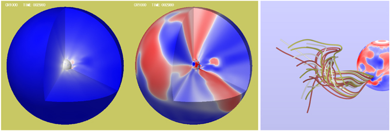
Figure 8. Left: simulated plasma density in the Sun-to-Earth MHD model on selected cutout planes (two meridional planes and a plane at 20° south), at  . Values are normalized by the density of the Parker solution; red, white, and blue show density ratios of 1.5, 1.2 and 1.0. Center: radial magnetic field component Br
normalized by the maximum absolute value at each radius. Blue (red) represents positive/outward (negative/inward) polarity. Right: selected field lines at
. Values are normalized by the density of the Parker solution; red, white, and blue show density ratios of 1.5, 1.2 and 1.0. Center: radial magnetic field component Br
normalized by the maximum absolute value at each radius. Blue (red) represents positive/outward (negative/inward) polarity. Right: selected field lines at  days in the scale of SMF modeling, or ∼0.4 days after eruption of a twisted magnetic structure began. The field lines are drawn for
  . The positive (negative) radial field Br
on the bottom-boundary sphere at 1.15
. The positive (negative) radial field Br
on the bottom-boundary sphere at 1.15  is colored blue (red). For visibility, the view point is 90° west of the left and middle cross-section plots.
Download figure:
Standard image High-resolution imageThe simulated eruption does not correspond to an actual solar event; hence, we do not claim accuracy for this simulation result. Instead, we emphasize the promise of connecting the global SMF model, with its powerful capability for handling nonpotential features in the lower corona, to the GHM model, with its capability to numerically simulate twisting coronal magnetic features at various spatial scales and trace their coronal and interplanetary consequences. We expect that such comprehensive modeling can be a foundation for further improvements and advances in operational space-weather modeling.
8. Discussion and Conclusion
We have presented an overview of the CGEM project to construct a framework for data-driven modeling to investigate the accumulation of magnetic energy that leads to eruptive events. The data driving is implemented through the PDFI electric field processing of the corrected HMI vector magnetograms, calibrated Doppler maps, and local correlation-tracking velocity fields. The time series of vector magnetograms and the resulting electric field maps make up the time-dependent boundary conditions that directly or indirectly drive the CGEM suite of numerical models: the global SFT model, the SMF model, the AR-scale radiative magnetohydrodynamic (RADMHD) model, and the global corona–heliospheric MHD (GHM) model. The CGEM MHD models were designed to start from either local or global SMF results and are driven by the same electric field formalism applied to the SMF simulation data. The PDFI electric fields have been made available to the community through the SDO JSOC.
The development of the CGEM framework represents a significant advance for numerical modeling of the dynamic, time-dependent solar corona. The incorporation of temporal sequences of photospheric vector magnetic field observations into the boundary conditions of large-scale and global modeling represents the most direct data-driving approach to date. While there are still improvements to be made in the treatment of the atmospheric evolution and for ensuring the self-consistency between the observed physical quantities and the time evolution of the full MHD system, the elements of the CGEM model now in place and available to the solar physics community enable systematic, quantitative investigation into the preeruption evolution and energization of active regions.
Understanding the physics of and being able to reasonably estimate the storage and release of free magnetic energy in the solar corona is one of the main challenges for the prediction of where and when solar flares and coronal mass ejections occur—which are some of the most important drivers of space weather for the Sun-to-Earth system.
The observed photospheric evolution of ARs and among AR systems can vary tremendously. In general, photospheric signatures of magnetic flux emergence, magnetic flux cancellation, and both large-scale and localized shearing and twisting motions are observed in ARs that range in complexity from simple, isolated bipolar regions to complex delta-spot configurations. While there has been a concerted effort to identify common signatures, or even statistical trends, in the preflare/preeruption evolution of ARs, the fact is that, often, each of these signatures is present at some time, or even simultaneously, during the AR lifetime. The CGEM PDFI approach of converting HMI vector magnetogram sequences into time series of electric fields suitable for incorporation into various numerical models means that these flows and the resulting physical quantities, such as the fluxes of magnetic energy and relative magnetic helicity into the corona, are readily available for essentially every active region observed in the SDO era. Additionally, utilizing the PDFI input in the data-driven SFT and SMF modeling yields critical information about the three-dimensional structure of these energized magnetic flux systems and the distribution of magnetic stress, electric currents, and other measures of nonpotentiality for the source regions of flares and CMEs.
The next major milestone in being able to predict—and realistically model—solar flares and CMEs is to understand their initiation process or processes. The rapid transition of sheared, twisted, and otherwise energized AR fields from a quasi-stable, quasi-equilibrium state to an unstable, runaway configuration that either drives or is driven by magnetic reconnection (or both), remains an important and active area of heliophysics research. The CGEM PDFI framework for direct data driving of numerical models of the solar corona is a critical component for furthering the theoretical development and understanding of AR stability and solar flare/CME onset. The SMF approach can identify the regions of concentrated shear/twist/nonpotentiality and quasi-unstable field regions in and around ARs. However, the diffusive "frictional" relaxation means the steep magnetic field gradients and strongly localized current densities required for the onset of fast magnetic reconnection are not resolved. Thus, a more complete physical model, i.e., the full MHD system, is necessary to resolve these structures and capture the impulsive nature of the onset and rapid reconfiguration of magnetic flux during eruption that converts the stored magnetic free energy into electromagnetic radiation, kinetic energy of the Alfvénic reconnection jets and erupting material, particle acceleration, and bulk plasma heating.
The PDFI electric-field-driving of the full MHD system, which ensures the model's physical consistency, continues to require further development, but also represents a necessary and promising avenue of future research. The 3D MHD evolution of the magnetic field state from the energized SMF configuration is one way to test the magnetofrictional instability thresholds for various ARs and determine just how important resolving the field/electric-current gradients are in determining the dynamics and evolution of the eruption onset and stable-to-unstable transitions. With the CGEM framework, we are now able to address a very interesting question: are the observed photospheric evolution (flows, emergence, cancellation) and the resulting estimate of energy accumulation sufficient to account for the observed energy release of a flare or CME event? If so, we are well on our way to a more realistic, physics-based modeling of the origin and evolution of energetic coronal transients. If not, there is something fundamental that our current observations and numerical models are missing. In either case, significant scientific progress can and will be made, our heliophysics modeling improved, and our space-weather forecasting capabilities advanced.
This work was supported by NASA and NSF through their funding of the CGEM project through NSF award AGS-1321474 to UC Berkeley, NASA award 80NSSC18K0024 to Lockheed Martin, and NASA award NNX13AK39G to Stanford University. This work was also supported by NASA through the one-year extension to the CGEM project, ECGEM, through award 80NSSC19K0622 to UC Berkeley. Some data products created for CGEM are available at the Solar Dynamics Observatory Joint Science Operations Center (SDO JSOC) supported by NASA contract NAS5-02139 (HMI) to Stanford University. W.P.A., D.J.B., B.J.L., and X.S. were funded in part by NASA grant NNX17AI28G. We wish to thank the US Taxpayers for their generous support for this project.
Footnotes
- 9
- 10
Also at 10.5281/zenodo.3939781.
- 11
- 12
- 13
- 14
To wit, by taking the divergence of Equation (2), one can show that
vanishes. Consequently, any field, even random noise, will render the net flux of Br
integrated over the full global SFT model unchanged from its initial value of zero. - 15
- 16


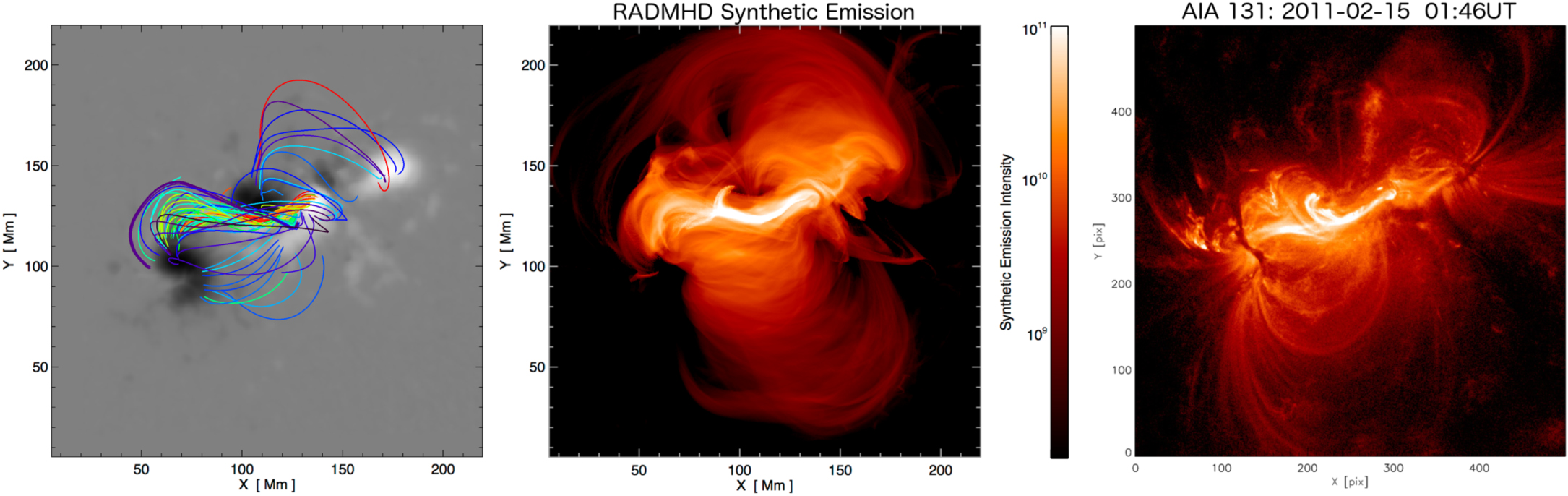
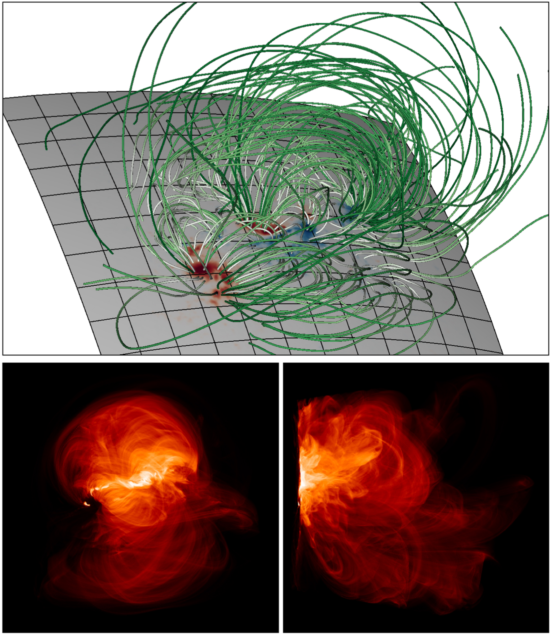