


Abstract
Interplanetary (IP) shocks are believed to play a significant role in both amplifying the background level of turbulent fluctuations and in heating the bulk solar wind (SW). This study investigates the thermodynamic properties downstream of IP shocks. We examine the temperature, density, and specific entropy changes in the shocked plasma, taking into consideration the geometric aspects of IP shock propagation within the expanding SW. Specifically, in our analysis, we account for the fact that any particular temporal range of one-point measurement may correspond to vastly different physically relevant temporal and/or spatial dimensions, such as the age of the shocked plasma and/or radial distance to the place where the plasma encountered the shock. Thus, our approach resolves the contradictions in previously reported temperature and specific entropy profiles in downstream regions and suggests that downstream regions exhibit greater turbulent heating compared to the pristine SW. This may contribute to the overall heating of the SW plasma. The paper presents a phenomenological parameter to predict specific entropy profiles and demonstrates the consistency of the proposed model with observations. We discuss the implications of these results for the thermodynamics of the SW beyond 1 au.
Export citation and abstract BibTeX RIS

Original content from this work may be used under the terms of the Creative Commons Attribution 4.0 licence. Any further distribution of this work must maintain attribution to the author(s) and the title of the work, journal citation and DOI.
1. Introduction
Thermodynamic properties of expanding solar wind (SW) plasma have been studied intensively for decades. The radial evolution of the temperature, density, and specific entropy of the SW fluid is complex and can be influenced by a wide variety of factors. While the density N is inversely proportional to the squared distance l from the Sun, N∝l−2, temperature and specific entropy exhibit nonadiabatic profiles (Whang et al. 1990; Adhikari et al. 2020a), i.e., there exists a source of free energy and this energy is dissipated by some process/processes, heating the SW fluid.
The two frequently invoked phenomena that provide sources of the energy around 1 au are (1) large-scale fluctuations of the magnetic and velocity fields and (2) the kinetic energy originating from the relative speeds of SW transients such as interplanetary coronal mass ejections (ICMEs) and interaction of fast and slow SWs. Regarding the latter source, the SW conditions favor a specific phenomenon that partially transforms the bulk kinetic energy (upstream) into the heat (downstream): a collisionless shock. The shock front, which is a region where irreversible entropy production occurs, is essentially a discontinuity; its thickness is of the order of the thermal gyroradius of the proton (Němeček et al. 2013), ρp, at 1 au ρp ∼ 100 km, while the spatial scale of the driver is of the order of astronomical units. Nevertheless, as the shock front propagates into the unshocked plasma, it can heat a significant portion of the SW (Whang et al. 1990), thus providing an additional source of heat distinct from the former turbulent energy source.
Previous studies have shown that the observations of the radial evolution of SW turbulence can be successfully explained in the framework of nearly incompressible (NI) MHD turbulence transport model in various plasma beta regimes (Zank & Matthaeus 1992; Zank et al. 1996, 2017; Hunana & Zank 2010; Adhikari et al. 2023). In general, these global physical models assume two sources of turbulent energy, (1) source related to the shears in the SW flow (and a simplified dimensional form of turbulence generated by shock waves) and (2) pick-up ion (PUI) driven turbulent fluctuations. Within ∼15 au, the former source dominates the PUI source (Zank et al. 1996, 2018; Zhao et al. 2017).
Apart from the two separate sources of heat/entropy enhancement in the SW fluid (turbulent cascade within pristine SW and MHD shock fronts), one can view the downstream shocked plasma regions (DRs) behind the shock fronts as another distinct region where the production of entropy can occur. The two distinct phenomena that give rise to DRs are ICMEs that drive a shock and SW stream interfaces that form a forward-reverse pair of shocks (Gosling 1996). Previous studies of interplanetary (IP) shock DRs focused mostly on the overall physical properties, such as the density, magnetic field, temperature, and various characteristics of the fluctuations of the magnetic field (Kilpua et al. 2017b; Richardson 2018; Borovsky 2020; Regnault et al. 2020; Zhao et al. 2021). Borovsky (2020) reported that DRs of IP shocks exhibit a constant profile of specific entropy and inferred that heating of the downstream plasma by a turbulence cascade at 1 au is thus not observed. On the other hand, Pitňa et al. (2021) suggested that both the increase in temperature and the turbulent cascade rate across the shock may influence the resulting downstream profile of temperature and specific entropy.
Recently, a number of studies focused on the interaction of turbulent fluctuations and MHD shocks from both theoretical and observational perspectives (Adhikari et al. 2016; Pitňa et al. 2017, 2021; Borovsky 2020; Zank et al. 2021; Trotta et al. 2022a; Park et al. 2023). In particular, Zank et al. (2021, hereafter Zank21) introduced a theoretical framework for the transmission of magnetic field fluctuations across highly perpendicular shocks with high upstream plasma beta values (β > 1). Pitňa et al. (2023, hereafter Pitňa23) showed that the enhancement of fluctuations across IP shocks at 1 au are consistent with the Zank21 theory, but the theory overestimates the downstream magnetic field turbulence level roughly by 30% on average. Their observations are consistent with previous findings that the energy within turbulent fluctuations decays with increasing downstream distance/time (Kilpua et al. 2013; Pitňa et al. 2017; Nakanotani et al. 2022) and neither of the aforementioned studies investigated the fate of the missing energy. A natural explanation is that it was transformed into heat. However, this explanation seems to contradict the findings of Borovsky (2020).
Concerning the changes of many distinct energy fluxes across the shock, some of the incident energy can be channeled into the production of energetic particles. The role of particle energization has been studied from observational (Dresing et al. 2016), numerical (Trotta et al. 2021), and theoretical (Leroy & Mangeney 1984) points of view. The energy flux of suprathermal and energetic downstream particles is typically ≲ 16% (David et al. 2022) of the total upstream energy flux. An analysis of terrestrial bow shock (BS) crossings by Magnetospheric Multiscale Mission shows that the majority of proton enthalpy flux is carried by a small fraction of suprathermal protons (Schwartz et al. 2022). On the other hand, Dresing et al. (2016) have shown, by examining a large set (475 cases) of IP shocks observed by twin Solar Terrestrial Relation Observatory that only a relatively small fraction of them exhibit significant enhancement of suprathermal (∼0.1 MeV) and energetic (∼2 MeV) particle fluxes. Studies by Zank et al. (2014, 2015), le Roux et al. (2015), Zhao et al. (2018, 2019) have shown that particle energization can take place further downstream of a shock front via the interaction of numerous small-scale flux ropes.
In this paper, we investigate again the temperature and specific entropy profiles from one-point spacecraft observations of DRs. Through superposed epoch analysis (SEA) of DRs, we show that the observed profile of specific entropy may exhibit decreasing, constant, or increasing trends. We suggest that DRs exhibit greater turbulent heating in comparison with pristine SW on average, which may contribute to the bulk heating of SW plasma beyond 1 au. In Section 2, we introduce physical considerations of the expanding SW, focusing on the evolution of the density, temperature, and specific entropy, and we derive a simple phenomenological parameter that qualitatively predicts the downstream profile of the specific entropy. In our analysis, we take advantage of the fact that DRs of IP shocks capture the radial evolution of the interaction of upstream SW plasma with the shock itself. In particular, we couple the changes of entropy in the preceding SW with the changes of entropy in DRs. In Section 3, we describe the statistical sample of IP shocks employed in the analysis. In Section 4, we show that our proposed phenomenology matches the observed profiles of DRs of IP shocks detected at 1 au consistently. Employing SEA, we show that the turbulent heating within DRs is larger than the corresponding upstream heating, which leads to an even more gradual decrease of the SW temperature with heliocentric distance. We expand on our results (derived from L1 observations) and we present implications for SW thermodynamics beyond 1 au. In Section 5, we discuss the validity of our assumptions made in the course of the analysis and present corresponding caveats. Finally, we present our conclusions and future plans.
2. Specific Entropy, Temperature, and Heating Rate
In this section, we introduce the thermodynamic considerations for the SW and IP shocks. We address the question of whether single spacecraft measurements of the DRs of IP shocks can be used to study turbulent processes. A key realization enabling us to infer physical insights about the DR is that the observation of downstream plasma can be viewed as a fossil record of the IP shock propagation through the expanding SW.
We introduce a physical picture that illustrates the problem of IP shock propagation. Let us assume adiabatic SW expansion so that the density Nu(l) ∝ l−2, temperature Tu(l) ∝ l−4/3, and velocity  . After the passage of an IP shock that propagates away from the Sun, the downstream plasma is heated and compressed. We suppose that (1) Nd(l) ∝ l−2, Td(l) ∝ l−4/3, and
  and (2) the density compression ratio, RN
, and temperature compression ratio, RT
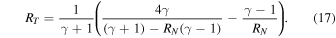
, across the shock do not depend on distance l, i.e.,
and (2) the density compression ratio, RN
, and temperature compression ratio, RT
, across the shock do not depend on distance l, i.e.,  and
and  . From an observational perspective, the key question that we address throughout the forthcoming analysis is: What profile of downstream temperature, specific entropy, and density would a spacecraft observe? It is clear that in this oversimplified picture, the spacecraft would observe constant N, T, and V.
We may invoke multiple phenomena that would considerably modify the above oversimplified model. Namely, (1) the pile-up of the plasma close to the driver of an IP shock (e.g., a magnetic cloud or ICME); (2) the decay/increase of shock strength with heliocentric distance due to an evolution of the shock driver, which leads to the radial changes of RN and RT ; (3) the nondiabatic radial temperature profile of the pristine and/or shocked SW. In the rest of the paper, we will focus our attention on the last phenomenon.
Now, let us assume that the upstream temperature follows  while Nu(l) ∝ l−2 and
  , and similarly, for the downstream we take
  , N(l)d ∝ l−2, and
  . We define the temperature excess, ΔTna−a, as the absolute change of the temperature (with respect to adiabatic expansion) that is required to satisfy the assumption T ∝ l−α
. It can be easily shown that, in order to observe a constant temperature profile at a fixed distance l, the following equality should hold:
. We define the temperature excess, ΔTna−a, as the absolute change of the temperature (with respect to adiabatic expansion) that is required to satisfy the assumption T ∝ l−α
. It can be easily shown that, in order to observe a constant temperature profile at a fixed distance l, the following equality should hold:  . This implies that the DR should exhibit even greater additional heating than the upstream region.
In the following paragraphs, we consider the thermodynamic relations for the specific entropy 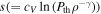 , where cV
is the specific heat per unit mass, Pth( = NkB
T) is the thermal pressure and ρ is the mass density. s is constant for adiabatic processes. However, observations show that the specific entropy of SW plasma increases with distance from the Sun (Whang et al. 1989; Adhikari et al. 2020a). Figure 1 introduces a visual diagram with which to consider entropy. The blue and red full circles mark the values of s
observed immediately upstream and downstream of an IP shock at distance l1, respectively. Straightforwardly, the increase of the specific entropy across the shock at l1 yields
, where cV
is the specific heat per unit mass, Pth( = NkB
T) is the thermal pressure and ρ is the mass density. s is constant for adiabatic processes. However, observations show that the specific entropy of SW plasma increases with distance from the Sun (Whang et al. 1989; Adhikari et al. 2020a). Figure 1 introduces a visual diagram with which to consider entropy. The blue and red full circles mark the values of s
observed immediately upstream and downstream of an IP shock at distance l1, respectively. Straightforwardly, the increase of the specific entropy across the shock at l1 yields
Note that ρu and  are connected to ρd and
  theoretically through the Rankine–Hugoniot (R-H) conditions. However, we can independently determine ρu,
  , ρd, and
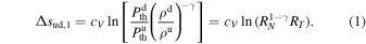
  from observations, without relying on the R-H conditions. Therefore, it is important to clarify that Equation (1) is not directly linked to the R-H conditions. Assuming no radial evolution of the shock, then, the increase of the specific entropy across the shock does not depend on distance, l, and we see that the increase of entropy at distance l0, Δsud,0, satisfies

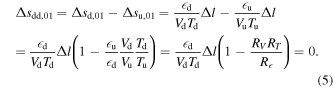
Further, we investigate the relation between the entropy of plasma immediately downstream of the shock at l1 (red circle) and the entropy of downstream plasma that have been detected also at l1 but it was shocked at l0 (orange circle). We denote the difference between these two levels of entropies as Δsdd,10. Note that this difference can be negative. If Δsdd,10 = 0, i.e., when the downstream entropy profile at l1 is constant, it would imply that Δsu,01 = Δsd,01, where Δsu,01 is the increase of entropy of the upstream plasma from l0 to l1, and Δsd,01 is the increase of entropy of the downstream plasma from l0 to l1. This in turn implies that the assumed power laws of the upstream and downstream radial temperature profiles would have the same exponents, which again implies  . In other words, if nonadiabatic heating of the upstream plasma increases its temperature by ΔT, then the nonadiabatic heating of downstream plasma must increase its temperature by RT
· ΔT. Thus, the heating rate of the downstream plasma must be higher than that of the upstream plasma. We derive an approximate formula that connects the enhancement of the heating rate with the entropy difference Δsdd,10 (see Table 1).
. In other words, if nonadiabatic heating of the upstream plasma increases its temperature by ΔT, then the nonadiabatic heating of downstream plasma must increase its temperature by RT
· ΔT. Thus, the heating rate of the downstream plasma must be higher than that of the upstream plasma. We derive an approximate formula that connects the enhancement of the heating rate with the entropy difference Δsdd,10 (see Table 1).
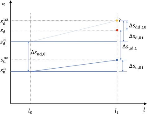
Figure 1. Schematic picture of the trends of the specific entropy with a distance from the Sun, l. For the sake of clarity, we list the definitions of various levels of specific entropy and their differences in Table 1. Here, we stress the meaning of the colored circles. Blue and red circles denote the values of the specific entropy immediately upstream and downstream of IP shock registered at a distance l1, whereas the orange circle marks the value of the specific entropy of the plasma that was shocked at distance l0, but detected later at distance l1.
Download figure:
Standard image High-resolution imageTable 1. Definitions of Various Specific Entropy Levels and Their Differences as Shown in Figure 1
| Quantity | Definition |
|---|---|

| Specific entropy of upstream IP shock plasma at distance l0 |

| Specific entropy of upstream IP shock plasma at distance l1 |

| Specific entropy of downstream IP shock plasma at distance l0 |

| Specific entropy of downstream IP shock plasma at distance l1, that have been shocked at l0 |
| sd | Specific entropy of downstream IP shock plasma at distance l1 |
| Δsu,01 |

|
| Δsd,01 |

|
| Δsud,0 |

|
| Δsud,1 |

|
| Δsdd,01 |

|
Download table as: ASCIITypeset image
Let us invoke the first thermodynamic law in the form,

where T denotes the temperature, s is the specific heat per unit mass,  is the dissipation rate per unit mass, and t is the time variable (Verma et al. 1995; Livadiotis et al. 2020). This simple equality shows that in order to increase the entropy of the plasma, dissipation of energy is required. We can rewrite Equation (3) as

where we used dl = Vdt.
We approximate the infinitesimal differential ds as  , and we express
  and
and  , where u and d are the upstream and downstream heating rates, Vu and Vd are the upstream and downstream SW speeds, Tu and Td are the upstream and downstream temperatures, and Δl = l1 − l0. Let us express the condition Δsdd,10 = 0 as
We define a ratio Rce as

which discriminates between three possibilities,


that correspond to three downstream entropy profiles at distance l1. The second case signifies the constant entropy, while the first/third determines the increase/decrease of the downstream entropy as it would have been measured by the spacecraft at a fixed distance from the Sun.
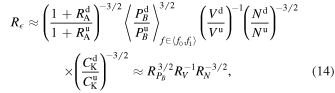
Finally, we discuss the heating rates in the upstream and downstream plasma. Considering the pristine upstream SW, the problem of SW heating has been intensively studied for decades (see, e.g., Bruno & Carbone 2013; Marino & Sorriso-Valvo 2023 and references therein). Here, we adopt a Kolmogorov phenomenology of SW turbulence (see, e.g., Vasquez et al. 2007; Smith & Vasquez 2021) and we model the heating rate as

where f denotes the spacecraft frame frequency, RA is the ratio of kinetic and magnetic energy (Alfvén ratio), PB is the trace of the magnetic field power spectrum and CK is an order of unity quantity.
2.1. Spacecraft Frame Time versus SW Distance
Spacecraft at a fixed distance from the Sun detect the incoming plasma with speed  , where tsp is the time in the spacecraft frame of reference. In a first approximation, the spatial scale δ
l which is sampled by the spacecraft within two times,
, where tsp is the time in the spacecraft frame of reference. In a first approximation, the spatial scale δ
l which is sampled by the spacecraft within two times,  and
and  ,
,  , can be estimated as δ
l = V · δ
tsp for the highly super-Alfvénic flow. Since the gradient of the SW speed outside ∼0.3 au is negligible (Durovcová et al. 2019; Adhikari et al. 2020b), one can use this simple formula for δ
l as large as ∼0.5 au.
, can be estimated as δ
l = V · δ
tsp for the highly super-Alfvénic flow. Since the gradient of the SW speed outside ∼0.3 au is negligible (Durovcová et al. 2019; Adhikari et al. 2020b), one can use this simple formula for δ
l as large as ∼0.5 au.
However, for the sub-fast magnetosonic speed flow observed behind the shock front at time  , one has to modify the calculation of the corresponding δ
ld. The key idea in the derivation is the transformation of the spacecraft spacetime
, one has to modify the calculation of the corresponding δ
ld. The key idea in the derivation is the transformation of the spacecraft spacetime  into the shock age time, tsh, which is defined as the time elapsed from the shock front encounter (Pitňa et al. 2017). The equation that connects tsh and
  reads as

where

where
V
d and Vsh denote the downstream SW velocity and shock speed in the spacecraft frame, respectively, and
n
is the shock normal. Finally, the distance, D, from the spacecraft to the point where the plasma encountered the shock, which has been observed at time  can be estimated as

Note that the factor K (Equation (12)) for IP shocks observed at L1 is ∼5.5–6 on average (Pitňa et al. 2017; Borovsky 2020), but it can reach values as low as 2 or as high as 15, implying that one has to carefully take into account this fact when comparing any quantities or their evolution within a fixed time window (e.g., δ tsp = 1 hr) for different shocks.
3. Data and Methods
In this study, we use a large set of fast-forward (FF) IP shocks observed by the Wind spacecraft between the years 1994 and 2017. We employ the Heliospheric Shock Database generated and maintained at the University of Helsinki. 5 The distance of the Wind spacecraft from the Sun is 1 au. Before 2004 May, the Wind orbit was complex and it was frequently located close to the Earth's BS. To exclude any possible foreshock activity in the data, we exclude IP shocks that were observed close to the BS, RWind < 50 RE, where RWind is the distance to the Earth's center and RE is the Earth's radius. Furthermore, we exclude IP shocks that follow another IP shock within 12 hr.
We use plasma measurements from the Solar Wind Experiment (SWE) and Magnetic Field Investigation (MFI) instruments (Lepping et al. 1995; Ogilvie et al. 1995). The sampling rates of the SWE and MFI instruments are 92 and 0.092 s, respectively. We analyze the proton density, velocity, and trace temperature, and we calculate the specific entropy for DRs of all IP shocks.
In estimating the heating rate of the upstream and DRs, we employ Equation (10) and estimate the trace power spectrum density PB
via continuous wavelet transform (Torrence & Compo 1998; Dudok de Wit et al. 2013). We are interested only in ratios of various quantities (see Equations (1) and (6)) and we approximate the ratio of the downstream to upstream heating rate R
as
where we defined the average ratio of the downstream to upstream power spectra,  in a frequency range bounded by f0 and f1 (covering a whole or significant part of the inertial range). We assumed that the change in the Alfvén ratio is small (Borovsky 2020) and that CK has the same or similar value in the upstream and downstream regions.
4. Results
The principal difficulty in the study of the DR lies in the fact that we do not know exactly the conditions of the plasma into which the IP shock propagates because it encounters SW plasma of different origins and the physical properties of particular plasma parcels can vary considerably. Furthermore, the shock key characteristics, such as its speed, Mach number, compression ratio, or obliquity respond to these changes in a complex manner. Furthermore, the shock front itself can vary locally from its mean structure, both as a result of (1) the shock front fluctuations in response to upstream turbulence/fluctuations (e.g., Zank et al. 2021; Trotta et al. 2022a, 2023b; Nakanotani et al. 2022) or (2) shock front rippling and reformation due to ion reflection and microphysical shock dissipation processes (see, e.g., Burgess & Scholer (2013), Kajdič et al. (2019), Gedalin et al. (2023), Trotta et al. (2023a), and references therein). Fundamentally, one-point measurements in the DR of a shock cannot differentiate between (1) changes induced by the varying upstream conditions and (2) changes in the shock parameters, which in turn leads to variability of the DR.
However, an SEA of the downstream profiles can partially overcome this difficulty. SEA has been widely used in many studies of space physics (see, e.g., Kilpua et al. 2017a; Borovsky 2020; Regnault et al. 2020). This simple, yet effective technique can reveal the systematic responses of complex physical systems. In our case, the system is the DR of IP shock. Motivated by the discussion in Section 2.1, we analyze the profiles of the density, temperature, and specific entropy, transforming the spacecraft time tsp into the distance D according to Equation (13).
Figure 2 shows an IP shock observed by Wind on 2000 July 19 at 15:30:24. This case illustrates the difficulties when analyzing any specific IP shock. The increase of s across the shock front is remarkably low (Δs = 0.15) in comparison with the relative differences on spatial scales of ∼10 minutes within the whole interval. The large increase of s, connected with a drop of the proton density and an increase of the temperature approximately 30 minutes behind the shock front (as well as the IMF discontinuity ∼40 minutes in the upstream) nicely illustrates the nonstationarity of the plasma into which the shock propagated on its journey to 1 au. One may easily argue that the increase of the specific entropy in the downstream from tsp = 0 to tsp = 2 hr is solely due to the changes induced at tsp ≈ 30 minutes.

Figure 2. Overview of the IP shock observed by the Wind spacecraft. From top to bottom, we plot the magnitude, ∣B∣, and components of the magnetic field, Bx , By, and Bz with black, blue, green, and red curves, respectively, in the GSE coordinate system, SW speed V, proton trace thermal speed Vth, proton density N, and specific entropy s. The time is centered on the passage of the shock front. The second X-axis in the bottom panel shows the corresponding distance from L1 toward the Sun at which the plasma encountered the shock (see Equation (13)). The vertical lines between D = 0 and D = 0.02 mark the interval within which the IP shock front adjacent median values of N, Vth, and s were estimated. The vertical lines between D = 0.18 and D = 0.2 mark the interval within which the median values of N, Vth, and s were estimated.
Download figure:
Standard image High-resolution image4.1. SEA
On using the shock parameters, Vsh,
n
, and average upstream/downstream plasma parameters, we estimate the following quantities: the K factor (Equation (12)) and spacecraft frame time,  corresponding to a distance D = 0.2 au (via Equation (13)),
  . The left and right panels in Figure 3 show the distribution of tD
and K, respectively. The average K of our sample yields
. The left and right panels in Figure 3 show the distribution of tD
and K, respectively. The average K of our sample yields  , a value slightly higher than that reported by Pitňa et al. (2017) and Borovsky (2020), and the average tD
is
, a value slightly higher than that reported by Pitňa et al. (2017) and Borovsky (2020), and the average tD
is  .
.

Figure 3. Left and right panels show the histograms of tD and K, respectively. Vertical dashed lines denote the median of the distribution.
Download figure:
Standard image High-resolution imageWe express the spacecraft frame time for downstream IP shock regions in a new dependent variable, D, according to Equation (13), and we analyze the superposed density, temperature, and specific entropy profiles up to D = 0.2 au.
Lastly, we estimate the ratio of downstream and upstream heating rates via Equation (14) for each shock by calculating the power spectral densities within one hour adjacent to the shock front in both upstream and downstream regions,  and
and  . The average ratio
  is estimated in the range of f0 = 0.01 and f1 = 0.1 Hz. Velocity and compression ratios (RV
and RN
) were calculated from the mean values of V and N over suitable 8 minute long upstream/downstream intervals.
6
is estimated in the range of f0 = 0.01 and f1 = 0.1 Hz. Velocity and compression ratios (RV
and RN
) were calculated from the mean values of V and N over suitable 8 minute long upstream/downstream intervals.
6
The left panel in Figure 4 shows the scatter plot of the observed values of R
as a function of RV
· RT
. We see that a majority of the values lie above R
/(RV
RT
) = Rce = 1. The right panel in Figure 4 shows the histogram of Rce; the median of Rce,  . On the basis of the analysis of the expected profiles of the specific entropy (see Section 2), we divide our statistical sample into three groups according to the estimated values of Rce,
- 1.Group (G1): Rce > 3
- 2.Group (G2): 3 > Rce > 0.3
- 3.Group (G3): Rce < 0.3.
The events corresponding to these groups are distinguished by colors in Figure 4, and the number of cases in groups G1, G2, and G3 are 35, 191, and 94, respectively.

Figure 4. Left panel shows the scatter plot of R
and the product RT
· RV
. The red, black, and blue colors mark the cases which belong to G1, G2, and G3, respectively. The right panel depicts the histogram of quantity Rce (see Equation (6)). The vertical dashed line denotes the median of the distribution.
Download figure:
Standard image High-resolution imageSince the time variable for s, N, and T is expressed in units of the distance D, we divide the D-axis equidistantly between D = 0 and D = 0.2 with ΔD = 0.02 and we estimate median values of s, N, and T within each bin. Note that the number of points used for the computation of medians within each bin can differ from case to case and from bin to bin because we analyze DRs with variable lengths and due to the rescaled data gaps.
For each case, we perform the following normalization. We divide the rescaled time series of N and T by the median values estimated between D = 0 and D = 0.02, i.e., by a value adjacent to the shock front. For the profiles of the specific entropy, we subtract the corresponding adjacent value. Finally, we show the median profiles of s, N, and T for each group (G1, G2, and G3) in the left, middle, and right panels of Figure 5, respectively. We can see that the SEA profiles of the density for each group are virtually the same and the natural explanation is that the functional form of the density profile  is the same in both the upstream and downstream regions, i.e.,
  . The right panel in Figure 5 shows that, unlike the density, the profiles of s for the subgroups are statistically different. For the group G1 (Rce > 3), the expected increasing trend (see Equation (7)) is consistent with the observed SEA profile, as are the expected constant and decreasing trends for the groups G2 and G3, respectively. As can be expected, the middle panel in Figure 5 shows the SEA profiles of T that are consistent with those of s. In terms of the differences in the functional forms of the radial temperature evolution between the upstream and downstream regions, the SEA profiles for the groups G1, G2, and G3 suggest that
  ,
,  and
and  , assuming that
  ,
,  and
and  , where superscripts u and d denote the upstream and downstream, respectively.

Figure 5. Left, middle, and right panels show the median SEA profiles of the normalized density, temperature, and specific entropy, respectively. The profiles are a function of the distance D (Equation (13)), i.e., an absolute distance of a plasma parcel with respect to L1. The plasma parcel is observed in the DR at L1, however, it was shocked closer to the Sun. In each panel, the red, black, and blue solid lines signify the profiles of IP shock groups G1, G2, and G3, respectively. The dashed curves mark the bootstrap-estimated errors of the corresponding medians. The X-axis is the distance from L1 along X-GSE.
Download figure:
Standard image High-resolution image4.2. Uncertainties of Rce and δ Sdd,01
In this section, we address the contribution of various errors/uncertainties that influence the SEA profiles. Generally, there are two sources of errors: (1) errors in the measurement of physical quantities of interest, N, T, V, B , and (2) the errors that arise due to the inherent variability of the turbulent fluctuations. We focus on the latter source, since their overall contribution is larger than the former.
In calculating the uncertainty of Rce, we employ the methodology of Pitňa23. Using Equations (14) and (6), we can express  . Pitňa23 showed that it is the variability of the upstream SW conditions that shapes the error distribution function of
  , exhibiting a strongly non-Gaussian character. Pitňa23 parameterized the spread of the distribution by a so-called central confidence interval factor (CIF), which is defined as the ratio of the upper and lower bound of the central confidence interval that contains 68.3% of values. This robust estimator of the width of a distribution characterizes the dynamic range of values of a random variable. As a proxy for
  for the ratio of the power spectra in this study, we use the value reported by Pitňa23,
  . If we assume that the uncertainties (in terms of CIF) of RN
and RT
are smaller than those of
. If we assume that the uncertainties (in terms of CIF) of RN
and RT
are smaller than those of  , then the desired CIF(Rce) can be estimated as
  . A straightforward numerical calculation yields CIF(Rce) ≈ 7.2. Furthermore, we estimate the CIF of the observed distribution of Rce, obtaining
  . We see that the dynamic range of observed values of Rce is larger than the dynamic range of the uncertainty, as can be expected. Considering these two estimates, they provide a reasoning behind the specific values of Rce that divide the whole set into three groups. Specifically, the upper and lower boundaries of Rce for the groups G1 and G3, respectively, are roughly equal to half of the dynamic range of the uncertainty of Rce, CIF(Rce)/2 ≈ 3.6 (with respect to Rce = 1).
Addressing the uncertainties of δ
sdd,01 is more involved. We focus on the entropy difference δ
sdd,01, between the last bin (D ∈ (0.18, 0.20)) and the bin adjacent to the shock front for each shock. This difference serves as a proxy for the change of entropy defined by Equation (5). In the right panel in Figure 7, we show the distribution of δ
sdd,01 (red curve). We estimate the standard deviation of δ
sdd,01,  . We argue that the scatter of δ
sdd,01 is given mostly by the variability of the pristine SW into which the shocks propagate. We can quantify this variability straightforwardly. First, we estimate the spatial dimension, δ
l, of the pristine SW that has been processed by the shock front as it propagated from 0.8 au up to 1 au (ΔD = 0.2) according to
. We argue that the scatter of δ
sdd,01 is given mostly by the variability of the pristine SW into which the shocks propagate. We can quantify this variability straightforwardly. First, we estimate the spatial dimension, δ
l, of the pristine SW that has been processed by the shock front as it propagated from 0.8 au up to 1 au (ΔD = 0.2) according to
Assuming an average SW speed of about Vsw,ave ∼ 500 km s−1, a rough estimate of the corresponding spacecraft frame time can be calculated simply as tp = δ
l/Vsw,ave, i.e., this estimates the typical time of the sweeping of a structure with dimension δ
l by a spacecraft. Figure 6 shows the distribution of tp for our set. The dashed vertical line denotes the median, med(tp) = 4.7 hr ≃ 5 hr. Next, we estimate the distribution of specific entropy differences, δ
s on the timescale δ
ts
= 5 hr. We employ the SWE Wind measurements between the years 1995 and 2022. For each year, we calculate the empirical distribution δ
s (see the right panel in Figure 7). The distributions δ
s and their moments exhibit solar cycle variation. Specifically, the standard deviation of δ
s, denoted as σδ
s
, is smaller around solar minimum and higher around solar maximum (see Appendix). Importantly, σδ
s
within 1995–2022 never exceeds 0.72. The median and average value of a set of standard deviations (28 values that correspond to 28 yr) yields  and
and  .
.

Figure 6. Histogram of tp for the entire set of IP shocks. The vertical dashed line denotes the median of the distribution.
Download figure:
Standard image High-resolution image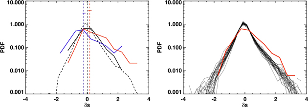
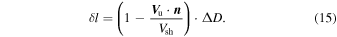
Figure 7. Left panel shows the PDFs of specific entropy increments δ s2010 (dashed black curve). The blue, black, and red curves denote the PDFs of δ sdd,01 for the groups G1, G2, and G3, respectively. The vertical dashed blue, black, and red lines mark the corresponding median values of the groups. Horizontal solid lines show the uncertainties of the medians. Right panel shows the PDF of δ sdd,01 for the entire set of analyzed IP shocks (solid red), while the black lines show the PDFs of specific entropy increments for each year between 1995 and 2022.
Download figure:
Standard image High-resolution imageIn the left panel of Figure 7, we show the distributions of δ
sdd,01 for G1, G2, and G3 with blue, black, and red lines, respectively. For illustration, we overplot the distribution of δ
s for the year 2010, δ
s2010. Complementary to the right panel in Figure 5, we show the median values δ
sdd,01 and their uncertainties for G1, G2, and G3 by dashed vertical and solid horizontal lines, respectively. While the three distributions overlap, we observe a consistent shift toward higher values of δ
sdd,01 as Rce increases, confirmed by the trends of the corresponding median values. The median values and their uncertainties for the groups G1, G2, and G3 read 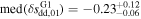 ,
, 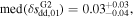 and
and 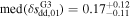 , respectively.
We suggest that it is the dependence of  on Rce that causes
  . Although we do not provide an explicit formula
 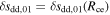 , which could be used to model the contribution of the true variation, we can roughly estimate the limiting value for
  , i.e., a situation when the downstream turbulent heating is insignificant with respect to the upstream heating. From Equation (5), we see that
 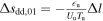 , i.e., the absolute value of the drop in the specific entropy Δsdd,01 is equal to the value of the increase in the specific entropy of the corresponding upstream pristine SW due to the turbulent heating on spatial scale δ
l (see Figure 1). Following Whang et al. (1990), we can roughly estimate the change in the specific entropy between 0.8 and 1 au as
7
, i.e., the absolute value of the drop in the specific entropy Δsdd,01 is equal to the value of the increase in the specific entropy of the corresponding upstream pristine SW due to the turbulent heating on spatial scale δ
l (see Figure 1). Following Whang et al. (1990), we can roughly estimate the change in the specific entropy between 0.8 and 1 au as
7
 , a value consistent with the median of δ
sdd,01 for Rce < 1/3 (group G3) in left panel in Figure 7 and right panel in Figure 5. Naturally, for Rce ≫ 1, one would expect that
, a value consistent with the median of δ
sdd,01 for Rce < 1/3 (group G3) in left panel in Figure 7 and right panel in Figure 5. Naturally, for Rce ≫ 1, one would expect that  . In other words, the enhancement of the specific entropy should be caused by the turbulent heating in the DR only. We conclude that Rce provides a good ordering of the observed changes in the specific entropy of the downstream plasma.
4.3. Implications for SW Heating beyond 1 au
In this section, we further elaborate on our findings and discuss the implications for SW heating beyond 1 au. We analyze observations at L1 and our analysis allows us to infer the changes in temperature/specific entropy within DRs on a spatial scale of ∼0.2 au. Since the median of Rce in our sample is ∼2, we suggest that the DRs exhibit stronger turbulent heating than the corresponding upstream plasma. Taking into consideration that the pristine SW exhibits a nonadiabatic profile of temperature  , αT > −4/3, it follows that the temperature profile in DRs is less steep,
  , αT,DR > αT. Consequently, this implies a more significant increase in specific entropy with heliospheric distance. It is evident that within and near 1 au, the influence on the overall temperature or specific entropy evolution is minimally affected since DRs constitute only a small fraction of the total SW mass. However, as the SW expands into the outer heliosphere, the role of stream interaction regions (SIRs) becomes increasingly important. Therefore, the physical processes within naturally occurring forward-reverse IP shock pairs beyond ∼1 au gradually exert a more substantial influence on the overall thermodynamic evolution of the SW.
A necessary condition for the excessive turbulent heating of DRs can be expressed as Rce(l) > 1. Here, we provide a phenomenological argument as to why such a condition is likely to be satisfied in the outer heliosphere. Starting with the definition of R
(see Equation (10)), we model the ratio of the downstream and upstream power spectra  by employing the turbulence transmission framework of Zank21. Assuming (1) quasi-perpendicular shock geometry and (2) fluctuation wavevectors lying in a direction parallel with the shock normal, the downstream wavevector kd and its fluctuation amplitude δ
Bd can be trivially expressed in terms of their respective upstream counterparts, ku and δ
Bu, as kd = RN
ku and δ
Bd = RN
δ
Bu. We approximate
by employing the turbulence transmission framework of Zank21. Assuming (1) quasi-perpendicular shock geometry and (2) fluctuation wavevectors lying in a direction parallel with the shock normal, the downstream wavevector kd and its fluctuation amplitude δ
Bd can be trivially expressed in terms of their respective upstream counterparts, ku and δ
Bu, as kd = RN
ku and δ
Bd = RN
δ
Bu. We approximate  as
as
where αB
denotes the spectral index of the spectra  and
and  , i.e., we assume
  . The extra factors RN
and αB
come from our desire to express
. The extra factors RN
and αB
come from our desire to express  at the same wavenumber k. Equation (16) expresses the upper limit for the theoretical enhancement of the power spectra.
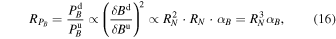
Next, we express RT as a function of RN using standard relations that couple the upstream and downstream thermal pressure and compression ratio (see, e.g., Zank21) as
For RN ≲ 2, this expression can be approximated as

Finally, we account for the weak dependence of RN on RV . For our statistical set, we found that

Using Equations (16), (18), and (19) allows us to approximate Rce as

We note that this approximation breaks down for RN ≳ 3 because the function RT (RN ) becomes highly nonlinear (its first derivative is highly dependent on RN for 3 ≲ RN < 4).
For moderate shocks (RN
≈ 2), assuming αB
= 5/3 and γ = 5/3, we obtain Rce ≈ 8, which is clearly an overestimate of the observed values within our set (recall that med(Rce) = 1.7). However, we focus on the strong dependence of Rce on RN
. Since the shocks associated with SIRs become stronger (RN
and their Mach numbers increase) with increasing heliospheric distance (Hoang et al. 1995; Pérez-Alanis et al. 2023), we suggest that Rce should increase with R, as long as RN
< 3. On the basis of the observations at ∼1 au (see Figure 5(c)), we suggest that Δsdd,01 > 0 for Rce > 1, implying that the observed DR IP shock profile would correspond to the situation when the downstream entropy change is larger than the upstream entropy change (see Equation (8)). In terms of temperature evolution, this would imply the following: if the upstream plasma exhibits a nonadiabatic radial temperature/entropy profile  with
with  , then the downstream plasma would follow
  with
with  . Although we do not provide a quantitative estimate for Δsdd,01 > 0, we suggest that the extra heating of DRs can partially explain the excess of specific entropy and temperature of SW protons observed between ∼ 5 and ∼ 15 au by Voyager 2 (see Figures 1 and 2 in Adhikari et al. 2020a).
5. Discussion and Conclusions
In this paper, we investigate the profiles of density, temperature, and specific entropy in DRs of FF IP shocks. Trivially, an IP shock increases N, T and s across the shock front. However, it is less obvious what the profiles of these quantities should look like further downstream in the spacecraft frame of reference. We suggest that the observed profile of specific entropy depends on the enhancement of temperature across the shock and on the increase of the turbulent heating rate from the upstream to downstream region. In the analysis, we made a number of simplifying assumptions, which we discuss further in the following paragraphs.
We made two crucial simplifications in the analysis: (a) the only source of energy that heats the upstream and downstream plasma is the cascaded turbulent energy and (b) all this energy is absorbed by the protons only. On the basis of numerous studies which investigate SW heating (Smith et al. 2001; Cranmer et al. 2009; Adhikari et al. 2017) and the partitioning of the cascading energy into protons and electrons (Howes 2010; Matthaeus et al. 2016; Roy et al. 2022), we suggest that both of these assumptions are well-supported. However, we acknowledge that the change in the ratio of heating rates of protons, Qp, and electrons, Qe, RQ
= Qp/Qe, may influence the results of our analysis, e.g., Matthaeus et al. (2016), Roy et al. (2022) have shown that RQ
scales with the sum Qp + Qe ∼ . Thus, the DR of IP shocks should exhibit larger proton heating. Furthermore, since the reported values of RQ
are generally larger than one for a plasma that exhibits proton–electron temperature anisotropy Tp/Te > 1, βp ∼ 1, proton heating within DRs should be larger than the electron heating on average.
Next, we explore our simplified perspective on the entropy change across the shock front. The problem of entropy generation and R-H conditions were discussed by a few authors in various contexts, namely, (1) variability of upstream/downstream polytropic indices (Livadiotis 2015; Scherer et al. 2016), (2) inclusion of PUIs and electrons into entropy jump calculations (Wu et al. 2009; Fahr & Siewert 2015), (3) effect of a nonthermal velocity distribution function f v in a form of κ-function (Livadiotis & McComas 2013) on the R-H conditions (Fahr & Siewert 2015; Livadiotis 2015, 2019), and (4) gyrotropic extension of fluid entropy (Du et al. 2020). Any of the listed points can be pursued further and could lead to a more detailed analysis of DRs. While we believe that a multi-fluid approach for the calculation of the entropy jump and its evolution inside DRs, together with empirical heating functions of protons and electrons, may improve the analysis outlined in this work, we leave this interesting and rather complex topic for future study. On the other hand, protons, as the primary ions in the SW, receive the majority of the turbulent heating and they are generally hotter than electrons. Therefore, it is reasonable for us to prioritize our focus on protons based on these factors.
We recognize that the statistical significance of median values of normalized T and s for distances 0.1 au ≲ D ≲ 0.2 au is weak. This is due to the fact that the 68.3% confidence regions for groups G1 and G3 only marginally deviate from the value δ
sdd,01 = 0, as depicted in the middle and right panels in Figure 5. However, given the substantial prior uncertainties associated with Rce and δ
sdd,01 and the sample sizes of the subgroups, these levels of statistical significance are expected. Indeed, if we crudely assume a normally distributed random variable G,  , we can roughly estimate the sample size NG
(number of independent draws from
, we can roughly estimate the sample size NG
(number of independent draws from  ) so that the standard error of the median value σmed of a random draw would be equal to μG
. Employing the relation between σmed and standard error of the mean value σmean,
) so that the standard error of the median value σmed of a random draw would be equal to μG
. Employing the relation between σmed and standard error of the mean value σmean,  (see, e.g., Maindonald & Braun 2010), and using expression
  , yields the formula
  . Calculation with μG
= Δs0.8→1 = − 0.18 and
. Calculation with μG
= Δs0.8→1 = − 0.18 and  , yields NG
≈ 21. This value is smaller but of the same order as the sample size of group G1, as expected. On the other hand, a similar calculation using σmed = μG
/2 and σmed = μG
/3 yields NG
≈ 60 and NG
≈ 130, respectively. These sample sizes are compatible with those of G3. Intriguingly, the middle group G2 exhibits a slightly increasing trend in s that can be considered as significant. We suspect that it is the distribution of the values of Rce within the ranges that define the group G3 that can explain this trend. We see that the majority of values of Rce are larger than 1. This feature is in accord with our hypothesis that Rce can well discriminate between the downstream entropy profiles (see Equations (6)–(9)). Importantly, the consistent trends observed in the (constant) density, along with the (decreasing/constant/increasing) trends observed in temperature and specific entropy across the entire range of investigated distances D for the three groups, provide compelling evidence.
, yields NG
≈ 21. This value is smaller but of the same order as the sample size of group G1, as expected. On the other hand, a similar calculation using σmed = μG
/2 and σmed = μG
/3 yields NG
≈ 60 and NG
≈ 130, respectively. These sample sizes are compatible with those of G3. Intriguingly, the middle group G2 exhibits a slightly increasing trend in s that can be considered as significant. We suspect that it is the distribution of the values of Rce within the ranges that define the group G3 that can explain this trend. We see that the majority of values of Rce are larger than 1. This feature is in accord with our hypothesis that Rce can well discriminate between the downstream entropy profiles (see Equations (6)–(9)). Importantly, the consistent trends observed in the (constant) density, along with the (decreasing/constant/increasing) trends observed in temperature and specific entropy across the entire range of investigated distances D for the three groups, provide compelling evidence.
Although our analysis does not depend on the validity of the R-H jump conditions, we discuss how common it is for IP shocks to comply with them. While it is generally accepted that for laminar low Mach number shocks, standard textbook R-H conditions capture the evolution of magnetic field and plasma parameters across the shock front, the situation is much more complex when the upstream medium contains some level of self-induced or preexisting population of magnetic field and plasma fluctuations (Trotta et al. 2022b; Gedalin 2023; Trotta et al. 2023a). The two mutually connected phenomena showing the complexity of the problem are the shock normal variability (connected to the shock rippling) and order-of-one fluctuations of the magnetic field (δ B/B0 ∼ 1) in upstream/downstream regions. For example, Gedalin (2023) investigated a special case of interaction of high Mach number quasi-parallel shocks with Alfvénic fluctuations, and derived a modified set of R-H conditions that couple the compression ratio, downstream root-mean-square magnetic field fluctuation and downstream pressure, implying that downstream turbulent magnetic field pressure influences the heating and compression across the shock. On the other hand, Zank et al. (2021) have shown that for a quasi-perpendicular shock interacting with a distinctly different kind of fluctuations (magnetic island mode), no modifications to R-H conditions are needed. In general, the variety of methods used in the determination of the key shock parameters, Alfvén and magnetosonic Mach numbers and angle θBn employ either a R-H shock fitting technique (Vinas & Scudder 1986; Koval & Szabo 2008) or a more direct approach of employing a coplanarity theorem and mass flux algorithm (Paschmann & Schwartz 2000). While these approaches are extremely useful in inferring the basic shock parameters, it is likely that for arbitrary oblique super-critical high Mach number shocks, an inclusion of magnetic and plasma fluctuations into a theoretical description may lead to modified R-H conditions.
In conclusion, we present a novel approach to analyzing the DRs of IP shocks using single spacecraft observations. We showed that the superposed profiles of density, temperature, and specific entropy are consistent with the view that SW turbulence heats predominantly protons in both the upstream and downstream regions. Due to the inherent geometry of IP shock propagation in the expanding SW and its consequent detection at a single distance from the Sun, single spacecraft measurements of DRs contain entangled information about the evolution of pristine/unshocked plasma and the evolution of the shocked plasma itself. We focus on the evolution of the specific entropy and we introduce a phenomenological parameter that couples the parameters of an IP shock and heating rates of the upstream/downstream turbulence. Using this parameter, we can discriminate between three basic scenarios: the entropy of a DR is decreasing/constant/increasing. We show that this parameter should increase as IP shocks propagate into the outer parts of the heliosphere, suggesting that the turbulent heating that takes place in DRs may contribute to the overall SW heating between ∼5 and ∼15 au. In a follow-up study, we plan to investigate the evolution of temperature and specific entropy in the framework of recently developed NI MHD turbulence transport models (Adhikari et al. 2023). Furthermore, a combination of such modeling with the novel IP shock observations through radially aligned spacecraft (such as Parker Solar Probe, Solar Orbiter, and/or L1 SW monitor) may help address the shock DR and how it evolves as it propagates to 1 au.
Acknowledgments
This work is supported by the Czech Grant Agency under contract (23-06401S). This paper uses data from the Heliospheric Shock Database, generated and maintained at the University of Helsinki. G.Z., L.Z., L.A., and M.N. acknowledge the partial support of NASA awards 80NSSC20K1783 and 80NSSC23K0415.
Appendix: Solar Cycle Dependence of Standard Deviation of Specific Entropy Differences
We analyze the differences in the specific entropy on a timescale of 5 hr for each year between 1995 and 2022. We employ Wind SWE measurements of proton density and trace proton temperature. Within each year, we estimate the empirical distribution of the differences of s, δ s, and we estimate its standard deviation, σδ s . The left panel in Figure 8 shows the variation of σδ s over two solar cycles and international sunspot number (ISSN) (Hathaway 2015). The right panel shows a modest correlation between σδ s and ISSN. Notably, during the years around solar minima, σδ s exhibits significantly lower values in comparison with the solar maxima.

Figure 8. The left panel shows the evolution of ISSN (black) and σδ s (red) between 1995 and 2022. The right panel shows the scatter plot of ISSN and σδ s . The value in the upper left corner is the Spearman's rank correlation between ISSN and σδ s .
Download figure:
Standard image High-resolution imageFootnotes
- 5
- 6
For details see http://ipshocks.fi/documentation
- 7
