


Abstract
The aim of this study is to compare observations of the magnetic field structure of observed quasi-parallel collisionless shock fronts with the results obtained analytically. A two-fluid analytic model of the shock front structure was derived under the assumptions that the shock is stationary and planar. The ion and electron kinetic pressures were assumed to be scalar, and polytropic state equations were used. The results of this analytical approach show that the shock magnetic field has an oscillatory structure. Venus Express (VEX) observations of the Venusian bow shock have been used to validate these theoretical findings. The Venusian bow shock and corresponding foreshock are significantly smaller than those of Earth. Thus, observations of the underlying structure of the quasi-parallel shock at Venus are not masked by the presence of high-amplitude waves and nonlinear structures originating in the foreshock. It is shown that the structure of the shock front, as observed by VEX, has a very strong similarity to the structure obtained analytically.
Export citation and abstract BibTeX RIS

Original content from this work may be used under the terms of the Creative Commons Attribution 4.0 licence. Any further distribution of this work must maintain attribution to the author(s) and the title of the work, journal citation and DOI.
1. Introduction
Collisionless shocks abound in the Universe. They are associated with gamma-ray bursts and appear in the vicinity of supernova remnants, ordinary stars, binary systems, and many other astrophysical objects. At present, collisionless shocks are regarded to be very efficient accelerators of charged particles. In many cases, the radiation generated by particles energized by collisionless shocks is a key source of information about the environment of a remote astrophysical object. A comprehensive understanding of the structure of the shock front and processes occurring there is crucial for the interpretation of this information. Currently, only collisionless shocks that occur within the heliosphere can be subjected to in situ measurements. While the majority of observations are made at the terrestrial bow shock, it is very important to study all other shocks in the heliosphere, to widen the range of environmental parameters and advance our understanding of collisionless shocks in the vicinity of distant astrophysical objects.
Shocks naturally occur in nature when a supersonic flow encounters an object in its path. In the case of a planetary bow shock, the object takes the form of either a magnetosphere, if the object possesses a natural magnetic field (e.g., Earth and Jupiter), or an "induced magnetosphere," if the object possesses an ionosphere but no intrinsic magnetic field (e.g., Venus). The two main parameters that are used for the characterization of collisionless shocks in the heliosphere are the Mach number (MA
Alfvénic or MF
fast magnetosonic) and the angle θBn
between the normal to the shock front
n
and the upstream magnetic field
B
u
. If the Mach number exceeds some critical value, then neither resistive nor dispersive processes are able to counterbalance the process of shock steeping and the process of ion reflection occurs to maintain a stationary shock front. In such strong, supercritical reflection shocks, θBn
is used to classify shocks as either perpendicular  , quasi-perpendicular
  , quasi-parallel
  , or parallel
  . Most of the ions reflected at the front of a quasi-perpendicular bow shock will be turned back toward the shock front under the influence of the upstream magnetic field. Thus, their motion will be restricted to a narrow region, known as the foot, whose width is on the order of half of the upstream ion convective Larmor radius. Various instabilities may operate in the foot, due to the presence of reflected ions. However, these instabilities will be confined to this relatively narrow region. In contrast, the ions reflected from a quasi-parallel shock are capable of traveling far upstream, forming an extended foreshock region. The simultaneous presence of reflected backstreaming and solar wind ions leads to the excitation of various plasma instabilities, resulting in the generation of plasma waves throughout the whole foreshock region. While these waves are propagating (and convected) in the foreshock, they are subjected to the same plasma instabilities, leading to their growth and the formation of nonlinear wave structures. The terrestrial foreshock is saturated with high-amplitude waves and nonlinear structures.
The Earth's bow shock results from the interaction between the supersonic flow of the solar wind with the terrestrial magnetosphere. The distance from the center of the Earth to the subsolar magnetospheric boundary is on the order of 10 Re (terrestrial radii), while that of the bow shock is about a couple of Re more distant. In contrast, at Venus, the position of the bow shock is much closer to the planet, due to the fact that Venus does not possess an intrinsic magnetic field, and so the Venusian ionosphere forms the obstacle to the solar wind flow (Zhang et al. 2008b). The distance to the subsolar point of Venusian bow shock from the center of the planet is about 1.5 Rv . By comparing the locations of Venus Express (VEX) crossings, Shan et al. (2015) determined that the subsolar stand-off distance varied within a solar cycle, being around 1.36 Rv during solar minimum and about 1.46 Rv at solar maximum. Because the planetary radii of both Venus and the Earth are similar, the typical stand-off distance of the Venusian bow shock is about an order of magnitude smaller than of the terrestrial bow shock. The close proximity of the shock to the planet translates into substantially shorter geometrical scales of the shock surface and the foreshock region. It is reasonable to expect that waves generated in the Venusian foreshock will have less time to interact with plasma instabilities, reducing their overall growth in comparison to waves generated within the foreshock at Earth. This should result in lower-amplitude plasma waves and nonlinear structures, and it may enable quasi-parallel shock observations that are not masked by a patchwork of nonlinear structures.
There is a distinct disparity between the numbers of observational studies of the structures of quasi-parallel and quasi-perpendicular shock fronts. Schwartz & Burgess (1991) analyzed data obtained by the AMPTE-UKS and AMPTE-IRM spacecraft in the vicinity of the terrestrial bow shock and concluded that the quasi-parallel region of the terrestrial bow shock was made up of a patchwork of three-dimensional, nonlinear structures, or SLAMS (Short Large-Amplitude Magnetic Structures). Since Schwartz & Burgess (1991), many studies based on in situ geospace data have studied the structure and dynamics of SLAMS as opposed to the structure of the quasi-parallel shock transition layer. This is probably due to the fact that the overall structure of the terrestrial quasi-parallel shock front is both hidden and modified by the existence of SLAMS according to Schwartz & Burgess (1991).
In this paper, a number of VEX observations of crossings of the quasi-parallel part of the Venusian bow shock are presented. All of these crossings display a shock transition layer that is not hidden by nonlinear structures formed in the foreshock. This allows them to be directly compared with theoretical models of the quasi-parallel shock front structure. It is shown that the theoretical models of the field structure within the front are in good agreement with the observations. This paper is structured as follows. Section 2 describes the data used in this study. Sections 3 and 4 present the observations of shock crossings. The development of an analytical model of a shock is presented in Section 5. Finally, in Section 6, the model and observations are compared and discussed.
2. Data and Instrumentation
The Venus Express spacecraft (VEX) had a highly elliptical orbit with a period of 24 hr. Its distance from the planet varied from about 66,000 km at apoapsis to a periapsis in the range 250–350 km (Zhang et al. 2006). The magnetic field measurements presented here were collected by the fluxgate magnetometer MAG (Zhang et al. 2006). Because VEX was not a magnetically clean spacecraft, MAG utilized measurements from two sensors at different distances from the spacecraft, to enable the automatic removal of interference resulting from the operation of the spacecraft (Pope et al. 2011). During most of the VEX orbit, MAG sampled the magnetic field at a rate of 1 Hz. However, during a two-hour period centered on periapsis, the sampling rate was 32 Hz. This study is based on observations using 32 Hz MAG data.
3. Shock Crossing on 2011 July 26 at 03:57 UT
The first shock crossing presented here occurred on 2011 July 26th at 03:57 UT and has been previously investigated by Shan et al. (2014). The three components (Venus Solar Orbital (VSO) coordinates) and the magnitude of the magnetic field are shown in Figure 1. The VSO coordinate system is planet-centered, with the X-axis directed toward the Sun, the Y-axis directed opposite to the Venus orbital velocity, and the Z-axis completing the right-handed triad. This is an outbound shock crossing that was observed soon after the detection of the ionopause at about 03:48:00 UT, as reported by Shan et al. (2014). As can be seen from Figure 1, the shock transition layer, highlighted by the gray shaded region between about 03:55:25 UT and 03:57:47 UT, is characterized by a decrease in the magnetic field magnitude from ∼20 nT to ∼8 nT. During this period, the spacecraft was located at ≈(8.12, 0.23, 4.1) · 103 km (VSO). Upstream of the shock, the spacecraft enters a region with significant wave activity with amplitudes of about 10 nT. However, the amplitude of these waves generally decreases with time such that, at around 04:07:00 UT, the wave magnitudes are only a few nT. Prior to the shock crossing, VEX observed multiple rotations of the magnetic field for about 6 minutes starting from 03:51:00 UT. The period of these rotations was around 20 s, during which the Y and Z magnetic field components oscillated in the range ±20 nT, exceeding the change of the magnetic field magnitude observed within the shock transition layer. During this period, the field magnitude remained constant at around 20 nT. The sharp decrease of their amplitudes in the upstream coincides with the decrease of the magnetic field magnitude. Shan et al. (2014) interpreted this feature of the shock crossing as the transmission of ULF waves through a shock front.

Figure 1. Three components and the magnitude of the magnetic field in the VSO coordinate system as observed during the Venusian bow shock crossing on 2011 July 26. The transition is highlighted by the gray shaded area.
Download figure:
Standard image High-resolution imageTwo methods, one based on minimum variance analysis (MVA) and the other on the model shape of the Venusian bow shock (Zhang et al. 2008a), have been used to identify the direction of the shock normal. Application of MVA to the 32 Hz full-resolution data for the interval 03:52:55.3–03:57:39.7 UT resulted in
n
MV ≈ [0.94, − 0.08, 0.34]. The ratios of the corresponding eigenvalues are  , providing a high level of confidence in the estimation of the minimum variance direction. In an attempt to remove any effects due to higher-frequency waves on the identified front normal direction, these data were smoothed using an 81 point moving average. Subsequent application of MVA to smoothed data resulted in a normal
n
MVs ≈ [0.95, − 0.06, 0.32]. The normal identified using the modeled shock surface (Zhang et al. 2008a) was
, providing a high level of confidence in the estimation of the minimum variance direction. In an attempt to remove any effects due to higher-frequency waves on the identified front normal direction, these data were smoothed using an 81 point moving average. Subsequent application of MVA to smoothed data resulted in a normal
n
MVs ≈ [0.95, − 0.06, 0.32]. The normal identified using the modeled shock surface (Zhang et al. 2008a) was ![${{\boldsymbol{n}}}_{\mathrm{mod}}\approx [0.96,\,-0.02,\,0.29]$](https://content.cld.iop.org/journals/0004-637X/959/2/130/revision1/apjad0b71ieqn6.gif) . All three identified directions for the shock normal are very similar. The angle between
n
MV and
n
MVs is less than 2°, while that between
n
MV and
. All three identified directions for the shock normal are very similar. The angle between
n
MV and
n
MVs is less than 2°, while that between
n
MV and  is ≈3
is ≈3 1. The upstream magnetic field has been estimated as the average over the time interval 04:04:50.5–04:09:46.1 UT
B
u
≈ [ − 6.38, − 0.72, − 1.87] nT. Comparison of these normal directions and the upstream magnetic fields reveals that the shock is quasi-parallel, because θBn
≈ 11°, ≈10°, and ≈7° for
n
MV,
n
MVs, and
1. The upstream magnetic field has been estimated as the average over the time interval 04:04:50.5–04:09:46.1 UT
B
u
≈ [ − 6.38, − 0.72, − 1.87] nT. Comparison of these normal directions and the upstream magnetic fields reveals that the shock is quasi-parallel, because θBn
≈ 11°, ≈10°, and ≈7° for
n
MV,
n
MVs, and  , respectively. These values are very similar to those obtained by Shan et al. (2014): 10° (MVA) and 4° (model).
Figure 2 shows the three components and the magnitude of the magnetic field in the shock coordinate system in which the n a -axis is directed along the front normal as determined using MVA, the l a -axis lies along the projection of the upstream magnetic field into the plane orthogonal to the n a -axis, and the m a -axis completes the right-handed triad. Again, the shock front transition region is highlighted in gray. To some extent, Figure 2 can be used to assess the validity of the identified shock normal. It can be seen that the Bn component does not exhibit any significant trend during the crossing of the shock transition layer 03:55:25–03:57:47 UT. In addition, the quasi-periodic oscillations with amplitudes exceeding 20 nT seen in the Bl and Bm components are absent in Bn . Morphologically, Figure 2 also indicates that the shock is quasi-parallel. The spacecraft took around two minutes to cross the shock transition region. This is significantly longer than can be expected for a crossing of a quasi-perpendicular shock magnetic ramp. The magnitudes of the waves and nonlinear structures observed in this particular foreshock region are significantly lower than those observed during a typical crossing of the terrestrial foreshock regions adjacent to the quasi-parallel shock front. Figure 3 shows a 3D plot of the evolution of the magnetic field in the plane orthogonal to the shock normal during the time interval 03:55:30–03:57:45 UT. The X-axis shows the time of observation and also gives an estimate of the distance of VEX from the time of the shock crossing (03:56:27), measured along the shock normal direction (assuming a stationary shock). It can be seen that the Bl and Bm components trace out a conical helix (conical spiral) along the time axis or a spiral in the plane orthogonal to the normal direction, with a radius that decreases as the spacecraft transits from downstream of the shock into the upstream region. The orthogonal magnetic field component rotations are almost circular in nature, as indicated by the similarity of the intermediate and maximum eigenvalues. Figure 3 displays four helical cycles observed between 03:55:30 and 03:57:00 UT. This period includes the time interval when ∣B∣ undergoes a transition between upstream and downstream values. More cycles, which are observed downstream of this transition region, are evident from Figure 2, but for the sake of clarity they are not displayed in Figure 3. From Figures 2 and 3, it is possible to estimate the spatial size of these oscillations. Within the transition region, the first and fourth peaks in the Bm component are observed at 03:55:36.4 and 03:56:33.0, respectively. During this period, the position of the spacecraft changes by about 300.5 km along the normal. Therefore, the spatial size corresponding to a single oscillation is approximately 100 km in the shock normal direction.

Figure 2. Three components and the magnitude of the magnetic field in the shock coordinate system, based on n MV as observed during the Venusian bow shock crossing on 2011 July 26. The gray shaded region marks the shock transition region.
Download figure:
Standard image High-resolution image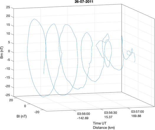
Figure 3. Three-dimensional plot of the evolution of the smoothed magnetic field component in the plane orthogonal to the shock normal B ⊥ = Bl l a + Bm m a , as observed during the Venusian bow shock crossing on 2011 July 26. The distance scale represents the distance from the shock (crossing time 03:56:27) along the shock normal direction.
Download figure:
Standard image High-resolution image4. Shock Crossings on 2011 December 15
The three VSO components and the magnitude of the magnetic field observed by VEX during the shock crossings on 2011 December 15 are shown in Figure 4. This is also an outbound passage of VEX during which the bow shock was crossed on three separate occasions. The spacecraft first entered the solar wind around 10:28:20 UT. About 3 minutes later, at 10:31:12 UT, the spacecraft crossed the shock for the second time, passing back into the downstream region. VEX finally crossed the bow shock for a third time at 10:32:24 UT, entering the region upstream of the shock. Each of these shock crossings will be discussed separately in the following subsections. These shock crossings were observed on the flank of the magnetosphere at an approximate location of ≈(− 1.57, 1.72, − 1.76) · 104 km (VSO), corresponding to a solar zenith angle of ≈120°.
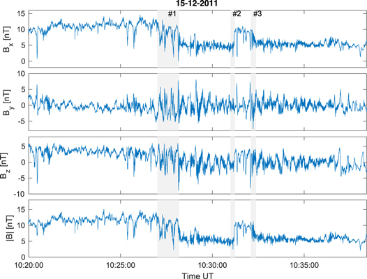
Figure 4. Three components and the magnitude of the magnetic field in the VSO coordinate system as observed during the Venusian bow shock crossing on 2011 December 15.
Download figure:
Standard image High-resolution image4.1. Shock Crossing 1 (10:28 UT)
The transition region associated with the first shock was encountered in the interval 10:28:02.4–10:28:15.2 UT. Using this period, MVA was used to determine the shock normal direction
n
MV ≈ [0.75, 0.44, − 0.50]. The ratios of the corresponding eigenvalues are  , again providing a high level of confidence in the estimation of the minimum variance direction. The upstream magnetic field
B
u
≈ [4.73, 0.02, − 0.5] nT has been estimated as the average over the time interval 10:29:32.1–10:31:02.4 UT. The corresponding angle between the shock normal and the upstream magnetic field is θBn
≈ 37°. While θBn
for this shock is significantly larger than for the previous shock discussed above, it is still considered as quasi-parallel.
, again providing a high level of confidence in the estimation of the minimum variance direction. The upstream magnetic field
B
u
≈ [4.73, 0.02, − 0.5] nT has been estimated as the average over the time interval 10:29:32.1–10:31:02.4 UT. The corresponding angle between the shock normal and the upstream magnetic field is θBn
≈ 37°. While θBn
for this shock is significantly larger than for the previous shock discussed above, it is still considered as quasi-parallel.
Figure 5 displays the magnitude and three components of the magnetic field in the shock coordinates system (Bn , Bl , and Bm ) for the shock crossing at 10:28 UT. It can be seen that ∣B∣ undergoes a change from ∼11 nT in the downstream at 10:28:06 UT to ∼5 nT on the upstream edge of the shock transition, shaded gray, at about 10:28:20 UT. Further validation of the identified direction of the shock normal is provided by the absence of significant changes or trends in the evolution of the normal component during this time interval. Oscillations in the Bl and Bm components are once again evident within the shock transition in Figure 5. These oscillations have some similarity with those observed at the shock 2011 July 26 discussed above. Their amplitudes decrease as the spacecraft travels from the downstream to the upstream region. The magnitude of the first oscillation encountered in the downstream region exceeds the 6 nT change in ∣B∣ observed in the transition region between the upstream and downstream. There is also one notable difference. The number of oscillations is smaller, and the time interval when they were observed is about 15 s and therefore much shorter than at the shock observed on 2011 July 26. Figure 6 shows a 3D plot of the evolution of the magnetic field in the plane orthogonal to the shock normal within the shock front transition region 10:28:03–10:28:18 UT. As in the previous case discussed above, the evolution of the magnetic field follows a conical spiral trajectory with the magnitudes of the almost circular rotations decreasing as the spacecraft travels upstream. However, only two large-magnitude oscillations are observed on the downstream side of the shock transition.
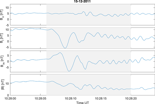
Figure 5. Three components and the magnitude of the magnetic field in the shock coordinate system, based on n MV as observed during the first Venusian bow shock crossing on 2011 December 15. The transition region is shaded in gray.
Download figure:
Standard image High-resolution image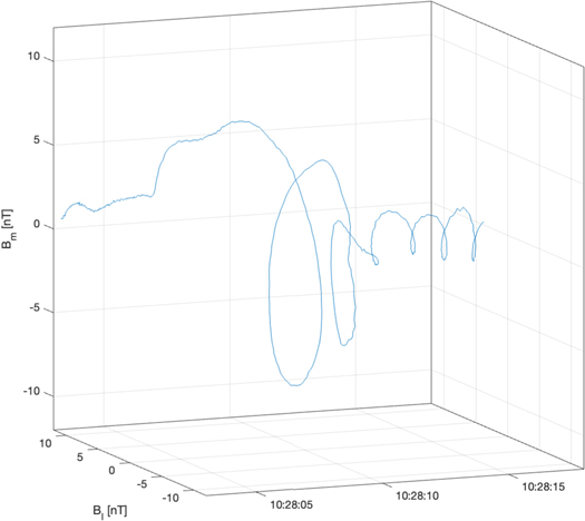
Figure 6. Three-dimensional plot of the evolution of the magnetic field component orthogonal to the shock normal B ⊥ = Bl l a + Bm m a , as observed during the first Venusian bow shock crossing on 2011 December 15.
Download figure:
Standard image High-resolution image4.2. Shock Crossing 2 (10:31:12 UT)
The changes in the shock frame components of the magnetic field for the second shock crossing observed on 2011 December 15 at 10:31:12 UT are shown in Figure 7. The shock transition is much shorter than that for the shocks discussed above. The normal direction, obtained using MVA, was
n
MV ≈ [0.63, 0.38, − 0.68] with eigenvalue ratios of  . Using the same upstream magnetic field determined above for the analysis of the first shock on this day, the angle between normal and upstream magnetic field was calculated to be θBn
∼ 46°. Ergo, this is an oblique shock that corresponds to the formal transition between quasi-parallel and quasi-perpendicular geometry.
. Using the same upstream magnetic field determined above for the analysis of the first shock on this day, the angle between normal and upstream magnetic field was calculated to be θBn
∼ 46°. Ergo, this is an oblique shock that corresponds to the formal transition between quasi-parallel and quasi-perpendicular geometry.

Figure 7. Three components and the magnitude of the magnetic field in the shock coordinate system, based on n MV as observed during the second Venusian bow shock crossing on 2011 December 15.
Download figure:
Standard image High-resolution imageFigure 8 shows the evolution of the magnetic field in the Bl , Bm plane. It can be seen that this shock does not exhibit high-magnitude oscillations within the region where ∣B∣ increases. This contrasts with the two previously discussed shock crossings. Only lower-magnitude oscillations, reminiscent of a whistler wave precursor, can be seen upstream of the transition region.

Figure 8. Three-dimensional plot of the evolution of the magnetic field component orthogonal to the shock normal B ⊥ = Bl l a + Bm m a , as observed during the second Venusian bow shock crossing on 2011 December 15.
Download figure:
Standard image High-resolution image4.3. Shock Crossing 3 (10:32:24 UT)
The shock frame magnetic field components and magnitude measured during the final shock crossing on 2011 December 15 are shown in Figure 9. As in the previous cases discussed above, the shock normal was determined by MVA to be
n
MV ≈ [0.85, 0.29, − 0.45] and the ratio of the eigenvalues was  . For this particular shock, the angle between normal and upstream magnetic field was computed to be θBn
∼ 32°, and thus the shock is quasi-parallel in nature. During the shock transition region, marked in gray, the magnitude of the magnetic field decreases by less than 5 nT. This shock crossing also exhibits a series of large (±5 nT) variations in the components of the magnetic field in the plane perpendicular to the shock normal direction, the sizes of which are comparable to or larger than the magnitude of the magnetic field change observed during the transition region. These variations are largest at the downstream edge on the transition region and become smaller as the satellite travels toward the upstream region, i.e., appearing as a conical helix. This evolution is clearly seen in Figure 10.
. For this particular shock, the angle between normal and upstream magnetic field was computed to be θBn
∼ 32°, and thus the shock is quasi-parallel in nature. During the shock transition region, marked in gray, the magnitude of the magnetic field decreases by less than 5 nT. This shock crossing also exhibits a series of large (±5 nT) variations in the components of the magnetic field in the plane perpendicular to the shock normal direction, the sizes of which are comparable to or larger than the magnitude of the magnetic field change observed during the transition region. These variations are largest at the downstream edge on the transition region and become smaller as the satellite travels toward the upstream region, i.e., appearing as a conical helix. This evolution is clearly seen in Figure 10.

Figure 9. Three components and the magnitude of the magnetic field in the shock coordinate system, based on n MV as observed during the third Venusian bow shock crossing on 2011 December 15.
Download figure:
Standard image High-resolution image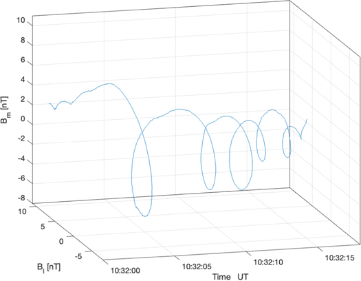
Figure 10. Three-dimensional plot of the evolution of the magnetic field component orthogonal to the shock normal B ⊥ = Bl l a + Bm m a , as observed during the third Venusian bow shock crossing on 2011 December 15.
Download figure:
Standard image High-resolution image5. The Upstream Magnetic Field from the Two-fluid Plasma Model
The upstream region of a supercritical collisionless shock may be affected by the reflected and backstreaming ions. Backstreaming ions are produced mainly in supercritical quasi-parallel shocks. They may cause instabilities and the generation of elliptically polarized waves well upstream of the shock transition. In low Mach number shocks, the number of backstreaming ions may be sufficiently low so as not to affect the upstream plasma. Low Mach number shocks in the heliosphere are also usually approximately planar and stationary. Based on these conditions and following Gedalin et al. (2015), two-fluid plasma theory should be an appropriate analytical approach to study the shock front structure. Within this approach, we consider a one-dimensional stationary plasma where all variables depend only on the coordinate x along the shock normal. Electrons are treated as a massless fluid. The ion and electron kinetic pressures are assumed to be scalar, and the polytropic state equations are used. Resistive dissipation is included as a friction term between the two fluids. Quasi-neutrality, ni = ne = n, is assumed, which is natural for the spatial and temporal scales under consideration. With these assumptions, the model equations take the following form:


where  is the unit vector along the x-axis,
  , and ⊥ denotes components perpendicular to
  .
E
and
B
are the total electric and magnetic field, respectively;
v
s
is the bulk velocity of the species s = e, i; ns
is the number density of the species s; and ps
is the pressure of the species s. The momentum exchange (friction between the electrons and protons) is described by the term ν. We have also taken into account that ni
=ne
implies vi
=ve
.
.
E
and
B
are the total electric and magnetic field, respectively;
v
s
is the bulk velocity of the species s = e, i; ns
is the number density of the species s; and ps
is the pressure of the species s. The momentum exchange (friction between the electrons and protons) is described by the term ν. We have also taken into account that ni
=ne
implies vi
=ve
.
In order to achieve better physical understanding, we introduce the following normalized variables:

allowing (1), (2), and (3) to be rewritten in the form of


where the subscript u denotes the asymptotically uniform upstream region, and

Here, nu
is the upstream number density, pu
is the upstream kinetic pressure, Vu
is the upstream plasma velocity along the shock normal  , mi
is the proton mass, e is the proton charge,
, mi
is the proton mass, e is the proton charge,  is the Alfvén speed, and M = Vu
/vA
is the Alfvénic Mach number.
is the Alfvén speed, and M = Vu
/vA
is the Alfvénic Mach number.
The dispersive length lw and the dissipative length ld are defined as follows:

where  and η is the resistivity. The length lw
is easily recognizable as the inverse wavenumber of a low-frequency whistler wave standing in the frame moving with velocity
and η is the resistivity. The length lw
is easily recognizable as the inverse wavenumber of a low-frequency whistler wave standing in the frame moving with velocity  .
.
The set of Equations (6), (7), and (8) cannot be solved analytically. For the numerical visualization shown below, we have chosen the fast magnetosonic Mach number MF
= 2 as fixed while θBn
and β are varied. A polytropic pressure is chosen, p(N) = NG
, with G = 5/3, so that  . The fast magnetosonic Mach number MF
= M(vA
/vF
), where
. The fast magnetosonic Mach number MF
= M(vA
/vF
), where
The ratio of the dissipation and dispersion lengths in terms of resistivity is
where Ωi
= eBu
/mi
c is the upstream proton gyrofrequency. For typical solar wind conditions, Vu
/c ∼ 10−3, one would have  . For the visualization below, we have chosen
  , which roughly takes into account the dependence of
  on the shock angle for constant resistivity. For the chosen parameters, the latter is in the range
  .
.
We solve Equations 6–8 numerically for x < 0, specifying boundary conditions for N, by , bz at x = 0. The equations are not valid in the region inside the ramp or downstream where kinetic effects are already important, so that the presented profiles describe the behavior of the magnetic field only upstream of the ramp. Figure 11 shows the magnetic profiles as a function of distance for cases when MF =2, β = 0.2, and for four values of the angle between the shock normal and the upstream magnetic field: θBn = 15°, 30°, 45°, 60°. The number of oscillations drops rapidly with the increase of the angle. Figure 12 shows a 3D plot of the evolution of the magnetic field component in the plane orthogonal to the shock normal for the analytical solution with θ = 15° and M = 2.01 in the same style as Figures 3 and 6. In Figure 12, the upstream plasma is hotter, β = 0.5, while MF and θBn are the same as in Figure 11. There is little difference between the behavior of the magnetic profiles for the same MF and θBn and different β. However, with the increase of β for given MF and θBn , the Alfvenic Mach number is higher. Respectively, the whistler wavelength is smaller.

Figure 11. The total normalized magnetic field b = ∣ B ∣/Bu (black line) and the two perpendicular components, bz = Bz /Bu (red) and by = By /Bu (blue). Top left: θBn = 60°, M = 2.13. Top right: θBn = 45°, M = 2.09. Bottom left: θBn = 30°, M = 2.05. Bottom right: θBn = 15°, M = 2.01. Other parameters: β = 0.2, MF = 2.
Download figure:
Standard image High-resolution image
Figure 12. Three-dimensional plot of the evolution of the magnetic field component orthogonal to the shock normal, for the analytical solution with θBn = 15° and M = 2.01.
Download figure:
Standard image High-resolution image
6. Discussion and Conclusions
For the quasi-parallel part of the terrestrial bow shock, the structure of the front may be concealed by the profusion of high-amplitude waves and nonlinear structures generated by various instabilities operating in the foreshock. At Venus, however, it is harder for the foreshock waves to reach similar amplitudes, simply because the smaller geometrical size of the Venusian foreshock implies that any waves would spend a shorter time among the instabilities that exist within the foreshock and therefore be limited in their growth. Therefore, at Venus, it is significantly easier to perceive the structure of a quasi-parallel shock, because it is not hidden by SLAMS or other waves/structures. The structure of the magnetic field for four bow shock crossings observed by the VEX spacecraft has been presented. For all of these shock crossings, the dynamics of the magnetic field throughout the shock transition in the plane perpendicular to the shock normal exhibit a conical helix or conical spiral evolution, with the amplitudes of the almost circular rotations increasing toward the downstream region (e.g., Figure 3). The center of rotation also changes as ∣B∣ increases within the shock transition layer. A shock structure resulting from two-fluid plasma theory exhibits very similar evolution of the magnetic field in the plane perpendicular to the shock normal within the shock transition layer (Figure 12). The good agreement between the observations and our theoretical model shows that the observed oscillations are not ULF waves transmitted through a shock front, as was suggested by Shan et al. (2014), but instead represent the internal structure of the shock transition layer.
The values of θBn for the four shocks observed by VEX are 11°, 32°, 37°, and 46°. Comparison of Figures 3, 6, 8, and 10 indicates that the number of rotations decreases as θBn increases. For the first shock discussed above, it was calculated that the spatial size of the observed oscillations is around 100 km along the shock normal direction. To allow a direct comparison with the numerical results shown in Figure 12, it is necessary to estimate the plasma dispersive length (Equation (11)). The estimation of the plasma dispersive length lw has been made based on the observations of the upstream magnetic field, together with typical values for the plasma density (10 cm−3) and velocity (400 km s−1). While these typical values for the plasma density and velocity may be different from reality, they are appropriate for the estimation of the order of magnitude of the dispersive length. These values yield an Alfvén velocity VA ∼ 34 km s−1, an ion inertial length c/ωpi ∼ 75 km, and a dispersive length lw ∼ 8 km. Thus, 100 km corresponds to ≈12 dispersive lengths. From the results of the numerical model for the case corresponding to θBn = 15° (lower right panel of Figure 11), we find that the wavelength of these oscillations is around eight dispersive lengths. This value is also in a good agreement with the observations. The main conclusion is that the VEX observations of the quasi-parallel shock front at Venus enable the identification of the structure of the magnetic field within the transition layer. This structure exhibits a conical helical evolution with the magnitude of the rotations increasing from the upstream to downstream.
Acknowledgments
M.A.B. and S.N.W. were supported by UK Natural Environment Research Council [NE/V002511/1]. M.G. was supported by the European Union's Horizon 2020 research and innovation program under grant agreement No. 101004131 (SHARP). M.A.B. and M.G. acknowledge support from the International Space Science Institute, Bern, Switzerland. The work of O.V.A. was supported by NSF grant No. 1914670 and NASA grants via contracts 80NNSC19K0848, 80NSSC22K0433, 80NSSC20K0218, 80NSSC22K0522, and 80NSSC20K0697. M.B. acknowledges helpful discussions with R. Drummond. Venus Express magnetic field data are available in the ESA's Planetary Science Archive (ftp://psa.esac.esa.int/pub/mirror/VENUS-EXPRESS/).