


Abstract
During the thirteenth encounter of the Parker Solar Probe (PSP) mission, the spacecraft traveled through a topologically complex interplanetary coronal mass ejection (ICME) beginning on 2022 September 5. PSP traversed through the flank and wake of the ICME while observing the event for nearly two days. The Solar Probe ANalyzer and FIELDS instruments collected in situ measurements of the plasma particles and magnetic field at ∼13.3 RS from the Sun. We observe classical ICME signatures, such as a fast-forward shock, bidirectional electrons, low proton temperatures, low plasma β, and high alpha particle to proton number density ratios. In addition, PSP traveled through two magnetic inversion lines, a magnetic reconnection exhaust, and multiple sub-Alfvénic regions. We compare these in situ measurements to remote-sensing observations from the Wide-field Imager for Solar PRobe Plus instrument on board PSP and the Sun Earth Connection Coronal and Heliospheric Investigation on the Solar Terrestrial Relations Observatory. Based on white-light coronagraphs, two CMEs are forward modeled to best fit the extent of the event. Furthermore, Air Force Data Assimilative Flux Transport magnetograms modeled from Global Oscillation Network Group magnetograms and Potential Field Source Surface modeling portray a global reconfiguration of the heliospheric current sheet (HCS) after the CME event, suggesting that these eruptions play a significant role in the evolution of the HCS.
Export citation and abstract BibTeX RIS

Original content from this work may be used under the terms of the Creative Commons Attribution 4.0 licence. Any further distribution of this work must maintain attribution to the author(s) and the title of the work, journal citation and DOI.
1. Introduction
Interplanetary coronal mass ejections (ICMEs) are macroscale structures of coronal plasma material and magnetic fields that drive space weather events and shape the heliosphere. ICMEs are one of the most energetic phenomena in our solar system and originate from the expulsion of coronal mass ejections (CMEs) from the Sun. There have been many proposed trigger mechanisms that eject CMEs from closed field lines on the Sun, such as magnetic reconnection (Gosling 1990). The occurrence rate of these eruptions has been shown to vary with the solar cycle (Webb & Howard 1994; St. Cyr et al. 2000), from less than one per day during solar minima, to a few events per day during solar maxima. Although white-light CME observations occur relatively frequently, the number of events that have been detected using in situ measurements is comparatively low. However, recently launched solar missions, such as Parker Solar Probe (PSP; Fox et al. 2016; Raouafi et al. 2023), provide in situ data much closer to the Sun to characterize the structure of CMEs at the early stages of their evolution.
The first spacecraft observations of CMEs can be traced back to the early 1970s when white-light coronagraphs on board the Orbiting Solar Observatory (OSO) and the Skylab space station revealed the presence of coronal transients (Tousey 1973). With the launch of the Solar Maximum Mission (SMM), the classical three-part CME structure was confirmed to have a bright frontal loop, dark cavity, and prominence core (Crifo et al. 1983; Illing & Hundhausen 1986). However, this structure is not universal, as some CMEs can be more complex. Narrow CME structures have been observed (Howard et al. 1985), either as narrow jets originating from coronal holes or narrow blobs from coronal streamers (Webb & Howard 2012). Other structures, such as Halo CMEs (Howard et al. 1982), appear large over a wide angular range as they primarily expand along the Sun–observer line.
In addition to remote-sensing observations, a number of in situ signatures have been identified for the detection of ICMEs, as compiled by Zurbuchen & Richardson (2006). It is important to note that none of these characteristics are necessarily guaranteed to be observed by a single spacecraft traveling through the event, owing to the inherent variability of each ICME (Gosling 1993). A certain group of ICMEs, known as magnetic clouds (MCs; Burlaga et al. 1981), are categorized by regions of smoothly rotating magnetic fields (≫30°) with a magnitude enhancement of at least 10 nT and low plasma β at 1 au (Klein & Burlaga 1982). MCs tend to have low proton temperatures Tp
, satisfying the condition  , where Texp is the expected proton temperature based on the solar wind (SW) speed relationship (Gosling et al. 1973; Richardson & Cane 1995). A significant difference between the expected and measured proton temperature may indicate solar wind plasma that has been perturbed by an ICME event or has experienced local compression or rarefaction. Cane & Richardson (2003) defined a quality index for MC identification, such that an index of two is assigned to ICME events that exhibit all typical features of MCs. An index of one indicates evidence of an MC solely based on magnetic field rotation, while an index of zero corresponds to events with no MC features. MCs are composed of a cylindrical bundle of twisted magnetic field lines with a helical structure, known as a flux rope (Burlaga et al. 1981; Klein & Burlaga 1982). Some MCs have been modeled with an elliptical cross section for the magnetic flux rope topology (Nieves-Chinchilla et al. 2018). While some of these characteristics have been observed separately for other macroscale structures in the solar wind, such as interplanetary sector boundaries (e.g., heliospheric current sheet (HCS) crossings; Schulz 1973; Bothmer & Schwenn 1992), they tend to simultaneously occur for MCs (Bothmer & Schwenn 1997). Other ICMEs may contain "complex ejecta" without flux ropes and typically have weaker magnetic fields and higher proton temperatures than MCs (Burlaga et al. 2001). However, MCs may appear as nonrope configurations in the case of a partial observation of the entire magnetic field structure (e.g., a spacecraft traveling through the legs of a flux rope).
Other in situ ICME signatures include directional discontinuities in the magnetic field around ICME boundaries (Janoo et al. 1998), fast-forward interplanetary shocks for fast ICMEs (Reames 1999; Manchester et al. 2012), and less magnetic field variation compared to ICME sheath regions (Klein & Burlaga 1982). At 1 au, enhanced alpha particle (fully ionized helium) to proton density ratios (>8%; Hirshberg et al. 1972) and periods of low density (<1 cm−3; Richardson et al. 2000) have occurred for ICME events. A monotonic decrease in solar wind velocity has also been reported after a sharp increase near the structure front (Klein & Burlaga 1982). The most common signature, valid for both slow and fast ICMEs, is the observation of bidirectional electrons above 80 eV (Gosling et al. 1987; Nieves-Chinchilla & Viñas 2008). The electron pitch-angle distributions (ePADs) typically show a single strahl beam directed along the magnetic field (Pilipp et al. 1987). The presence of bidirectional electrons (i.e., electrons streaming both parallel and antiparallel to the magnetic field) may indicate a connection to both foot points on the Sun from closed field line loops within ICMEs.
The scope of this study encompasses a time interval of nearly two days, from 2022 September 5 to September 7, as PSP traversed an ICME at ∼13.3 solar radii. This event provides an unprecedented opportunity to study the plasma and field structures of an ICME in detail at an early stage of its evolution. PSP observed the flank and wake regions of the ICME, providing novel observations compared to measurements near 1 au. We focus primarily on PSP in situ measurements—the mission does offer remote-sensing capabilities that are discussed in greater detail elsewhere (e.g., A. Vourlidas et al. 2023, in preparation). The event included a combination of several interesting features related to classical ICME in situ signatures (described above) that have not previously been observed by PSP. Section 2 provides a summary of the in situ data, highlighting important features and time intervals related to the ICME. Section 3 presents the CME model from C. R. Braga et al. (2023, in preparation) along with white-light coronagraph observations. An animation of the model is shown to synchronize the remote-sensing observations, in situ measurements, and modeled CME propagation over time, providing a comprehensive visualization of the event. Section 4 uses Potential Field Source Surface (PFSS) modeling and in situ data to investigate the source region and large-scale coronal structure before and after the event. Finally, Section 5 compares PSP observations with CME modeling and coronal magnetograms to offer insight into the ICME structure and evolution.
2. PSP in Situ Measurements
2.1. Instrumentation
The PSP mission was launched in 2018 August 12 to collect unprecedented in situ measurements of the solar wind close to the Sun (Fox et al. 2016; Raouafi et al. 2023). The main science goals are to study the Sun's lower coronal structure, solar wind heating and acceleration, and energetic particle acceleration. The spacecraft orbits the Sun in a highly elliptical trajectory, using Venus gravity assists in gradually decreasing its perihelion distance from 35.7 to 9.9 solar radii (RS ) over the course of the prime mission. During each encounter phase, the instruments on board PSP collect measurements of solar wind plasma ions and electrons, magnetic and electric fields, and energetic particles, as well as white-light images off-disk. The orbital perihelion for the thirteenth PSP encounter, which is the focus of the present paper, was reached on 2022 September 6, with a closest approach of 13.3 RS .
For this study, we use data from the Solar Wind Electrons, Alphas, and Protons (SWEAP; Kasper et al. 2016) suite. SWEAP consists of two electron electrostatic analyzers collectively known as Solar Probe ANalyzer for Electrons (SPAN-E; Whittlesey et al. 2020), one ion electrostatic analyzer referred to as the Solar Probe ANalyzer for Ions (SPAN-I; Livi et al. 2022), and a Faraday Cup called the Solar Probe Cup (SPC; Case et al. 2020). SPC was powered off for most of the period of interest due to temperature constraints. Thus, the proton and alpha particle parameters in this study, i.e., number density n, temperature T, and velocity v , are estimated exclusively from the SPAN-I moments. To obtain electron plasma parameters, we follow a similar method from Halekas et al. (2020) with a few minor differences. An anisotropic bi-Maxwellian distribution is fitted to the core electron population along all pitch angles using SPAN-E three-dimensional electron velocity distributions. We have recomputed the anode efficiencies for both SPAN-E instruments to match the plasma density calculated from other onboard instruments, discussed below. Below ∼25 eV, the SPAN-E instruments are contaminated by secondary electrons and photoelectrons. We determine the local minimum between the secondary and core electron distributions and fit the core from this minimum to the peak of the distribution.
We also utilize Level 2 magnetic field data from the fluxgate magnetometer in radial–tangential–normal (RTN) coordinates at ∼4 samples per second from the FIELDS suite (Bale et al. 2016). The RTN coordinate system is defined as: R is directed away from the Sun to the spacecraft, T is tangential to the spacecraft orbit, and N is normal to the RT plane (Fränz & Harper 2002). FIELDS measurements are used to study the background magnetic field structure and calculate ePADs. For comparison with the SPAN-derived plasma densities, we calculate the quasi-thermal noise (QTN) total electron density using the Radio Frequency Spectrometer (RFS) from the FIELDS suite, specifically the Low Frequency Receiver (LFR) data from the V1–V2 and V3–V4 antenna dipole pairs (Pulupa et al. 2017). We implement a new simplified heuristic algorithm to calculate the QTN electron density, described in Appendix A. We find the density derived from this method agrees with the QTN electron density from Moncuquet et al. (2020) within 5%–10%, and the electron core density within 5%–15% near each encounter.
2.2. Overview of in Situ Observations
Figure 1 presents an overview of the encounter 13 ICME event between 2022 September 5 and September 7. The first panel shows three different plasma densities n computed from QTN (black), SPAN-E core electron fits (red), and SPAN-I proton moments (blue). The second panel displays the bulk SW speed ∣
v
∣ from SPAN-I moments for protons (blue) and alpha particles (green). Core electron (red), proton (blue), and alpha particle (green) temperatures are shown in the third panel. We compute an expected proton temperature (magenta) to compare with Tp
as measured by SPAN-I (see Appendix B for details). The next panel shows the alpha particle to proton number density ratio na
/np
, with a dashed horizontal line indicating the typical fast solar wind value of 4%. Figures 1(e) and 1(f) display the Alfvén Mach Number ( ), and electron (red) and proton (blue) plasma β (
β
s
= 8π
ns
kTs
/B2 for species s), where the horizontal dashed lines are set to 1. The QTN electron density measurement is used for both βe
and βp
calculations, as the absolute accuracy of this method is superior and quasi-neutrality of the plasma may be safely assumed. While np
is replaced by the QTN electron density for βp
(which includes a small alpha particle density portion), the proton temperature is used to compute βp
. The next panel shows the differential energy flux (Eflux) spectrogram, with units of eV s−1 cm−2 ster eV−1, for protons summed over all field of view (FOV) angles measured by SPAN-I. Figure 1(h) depicts the magnetic field data in RTN coordinates from FIELDS. The bottom panel shows ePADs measured at 433 eV from SPAN-E, normalized to the differential energy flux average for each sample. This energy band is selected as the peak of the strahl distribution tends to be within ∼300–500 eV. The vertical dashed lines represent different time intervals when the plasma parameters display significant changes or interesting features. These intervals are summarized in Table 1, with a lettered label for each subinterval. Remote-sensing observations from PSP and other spacecraft, described in Section 3, indicate that the CME eruption became visible near time t0 (2022 September 5 at 16:10 UT).
), and electron (red) and proton (blue) plasma β (
β
s
= 8π
ns
kTs
/B2 for species s), where the horizontal dashed lines are set to 1. The QTN electron density measurement is used for both βe
and βp
calculations, as the absolute accuracy of this method is superior and quasi-neutrality of the plasma may be safely assumed. While np
is replaced by the QTN electron density for βp
(which includes a small alpha particle density portion), the proton temperature is used to compute βp
. The next panel shows the differential energy flux (Eflux) spectrogram, with units of eV s−1 cm−2 ster eV−1, for protons summed over all field of view (FOV) angles measured by SPAN-I. Figure 1(h) depicts the magnetic field data in RTN coordinates from FIELDS. The bottom panel shows ePADs measured at 433 eV from SPAN-E, normalized to the differential energy flux average for each sample. This energy band is selected as the peak of the strahl distribution tends to be within ∼300–500 eV. The vertical dashed lines represent different time intervals when the plasma parameters display significant changes or interesting features. These intervals are summarized in Table 1, with a lettered label for each subinterval. Remote-sensing observations from PSP and other spacecraft, described in Section 3, indicate that the CME eruption became visible near time t0 (2022 September 5 at 16:10 UT).

Figure 1. Time series of the encounter 13 ICME event observed by PSP. (a) QTN electron (black), proton (blue), and core electron (red) density, (b) proton (blue) and alpha particle (green) bulk speed, (c) proton (blue), alpha particle (green), core electron (red), and expected proton (magenta) temperature, (d) alpha particle to proton number density ratio, (e) Alfvén Mach number, (f) proton (blue) and electron (red) plasma β, (g) proton differential energy flux spectrum with units of eV s−1 cm−2 ster eV−1, (h) RTN magnetic field with magnitude (black), (i) normalized electron pitch-angle distribution at 433 eV. The heliocentric distance of PSP in RS is shown at the bottom along the time axis. The light and dark orange shaded regions depict intervals when ions or alpha particles are outside of the SPAN-I FOV or energy range, respectively. The vertical dashed lines represent different time intervals when the plasma parameters display significant changes or interesting features, corresponding to the intervals in Table 1. The subinterval labels are not shown.
Download figure:
Standard image High-resolution imageTable 1. Time Intervals of ICME Event
| Time Interval | Start Time (UTC) | In Situ Signatures | ICME Feature |
|---|---|---|---|
| t0 | 22-09-05/16:10:00 | Remote-sensing Observations | CME Eruption Visible |
| t1 | 22-09-05/17:27:20 | n, v, T, & B increase ∥ 90° ePADs | ICME Shock |
| t2a | 22-09-05/17:33:04 | Diffuse ePADs ∥ Smooth B | End of Sheath |
| t2b | 22-09-05/18:02:26 |

| ICME Flank |
| t3a | 22-09-05/19:08:46 | Bidirectional ePADs ∥ B rotations | Closed Field Lines |
| t3b | 22-09-05/19:49:23 |
 ∥ n < 103 cm−3 ∥ n < 103 cm−3
| |
| t4a | 22-09-05/20:09:05 | n ≫ 103 cm−3 ∥ B rotation | First Inversion Line |
| t4b | 22-09-05/21:19:06 |
 ∥ ePAD inversion ∥ ePAD inversion | |
| t5a | 22-09-06/01:14:17 | v & T decrease | Exiting ICME Plasma |
| t5b | 22-09-06/03:26:00 | Stable plasma conditions | Typical SW |
| t6 | 22-09-06/08:39:49 | MA < 1 ∥ Diffuse ePADs | Sub-Alfvénic Region |
| t7a | 22-09-06/17:27:28 | MA > 1 ∥ ePAD inversion | CS Leading Edge |
| t7b | 22-09-06/17:40:00 | MA ≪ 1 | CS Trailing Edge |
| t8 | 22-09-07/06:11:28 | MA increase | |
| t9 | 22-09-07/11:30:16 | Pre-event SW conditions | End of Event |
Note. Selected time intervals during the encounter 13 ICME event. Some intervals are divided into subintervals, denoted by a lettered subscript. The plasma signatures described in the table represent the most significant in situ observations for each interval and correspond to an ICME feature.
Download table as: ASCIITypeset image
The SPAN-I sensor is mounted behind the thermal protection of PSP and therefore does not have a direct view of the Sun line. The gap in the SPAN-I FOV is mostly apparent at far heliocentric distances, where the spacecraft velocity is slow (relative to perihelion) and the solar wind appears more radial in the spacecraft frame. As the spacecraft approaches perihelion, the aberration between the SW velocity and spacecraft velocity becomes large enough to measure the full three-dimensional velocity distribution function (VDF). The transition between regimes is variable and depends on local solar wind conditions. The light and dark orange shaded regions in Figure 1 depict intervals when either ions or alpha particles are outside of the SPAN-I FOV or energy range. During this event, the proton VDF moved out of the SPAN-I FOV and briefly out of the instrument energy range above 20 keV.
2.3. ICME Shock Analysis
Figure 2 shows a magnified time series from time intervals t1 (17:27:20 UTC) to t4 (20:09:05 UTC) with similar panels to Figure 1. In addition, Figure 2 includes normalized ePADs measured at 1152 eV, and the magnetic field elevation angle θB and azimuthal angle ϕB . The magnetic field angles have been smoothed over an averaging window of 5.5 minutes to focus on large-scale rotations in B . At time t1 on 2022 September 5, the electron number density ne is measured to abruptly increase from about 1880 to 4000 cm−3, followed by a gradual decrease below 1000 cm−3. The bulk speed ∣ v ∣ sharply increases from ∼340 to 650 km s−1 and continues to grow until 1350 km s−1. The proton temperature Tp surges from 65 to 520 eV with a subsequent increase to 2 keV. The magnetic field magnitude B abruptly strengthens from approximately 625 to 1500 nT and continues to about 1650 nT. These values of n, v, T, and B downstream of the discontinuity are not typical at these solar distances based on previous PSP encounters. This may indicate that PSP has encountered a compression region. In addition, PSP observes the magnetic field to become more turbulent after t1, along with an increase in higher-energy protons (E > 3500 eV, see Figure 1(g)) and electrons (E > 350 eV, not shown).
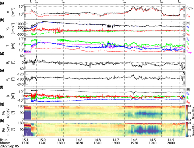
Figure 2. Time series from 17:20 to 20:15 UTC on 2022 September 5 as observed by PSP. (a) QTN (black) and core (red) electron density, (b) RTN proton velocity with magnitude (black), (c) proton (blue), alpha particle (green), core electron (red), and expected proton (magenta) temperature, (d) magnetic field elevation angle, (e) magnetic field azimuthal angle, (f) RTN magnetic field with magnitude (black), and normalized ePADs measured at (g) 433 eV and (h) 1152 eV. The magnetic field angles have been smoothed using a moving average of 5.5 minutes. The heliocentric distance of PSP in RS is shown at the bottom along the time axis. The vertical dashed lines represent different time intervals, corresponding to the intervals in Table 1, from t1 to t4a .
Download figure:
Standard image High-resolution imageTo estimate the orientation of the leading discontinuity at time t1, we perform a shock geometry analysis using measurements from PSP. We implement a standard single-spacecraft analysis of the magnetohydrodynamic (MHD) Rankine–Hugoniot (RH) jump conditions across the discontinuity to derive the most probable shock plane propagation vector using the methods described in Viñas & Scudder (1986), Szabo (1994), and Koval & Szabo (2008). The sampled upstream and downstream in situ measurements from PSP represent the slab-symmetric asymptotic conditions. Using the pre-shock and post-shock conditions, the shock orientation and speed are determined based on the optimal solution that satisfies Maxwell's equations and the conservation of mass, momentum, and energy across the discontinuity. The RH equations will yield a unique and robust solution if the bootstrap analysis consistently approaches the same solution. The model assumes ideal MHD, thermal isotropy, and equal partitioning of pressures between ions and electrons. As none of these are strictly true, we expect only a rough estimate for the shock solution from this exercise.
The upstream and downstream plasma parameters near time t1 are described in Table 2, averaged ∼60 and 30 s before and after the discontinuity, respectively. These include the RTN velocity v RTN, RTN magnetic field B RTN, proton scalar thermal speed ωp , and electron number density ne . The associated uncertainties are based on the ensemble of outcomes from sampling the upstream and downstream conditions. We find a fast-forward shock solution of cross-boundary flow with a Fast Mode Mach number transition from 2.40.1 on the upstream side to 0.650.03 on the downstream side. The most probable shock orientation is found to be significantly nonradial, with a propagation vector directed −51° ± 4° from +R in the RT plane and 23° ± 3° from +R in the RN plane. The most probable propagation speed is estimated as 1002 ± 30 km s−1 in the SW frame. Figure 3 illustrates this inferred shock geometry with the orbital trajectory of PSP for encounter 13 in Heliocentric Earth Equatorial (HEEQ) coordinates. The portion of the orbit from times t1 to t9 listed in Table 1 is highlighted in orange. The HEEQ coordinate system is defined with the x-axis directed toward the intersection between the solar equator and solar central meridian of date and the z-axis toward the solar rotation axis (Fränz & Harper 2002). PSP is located in its orbit at time t1, with the projected shock plane and normal in red. The black dashed line in Figure 3 represents the eruption axis of the event, aligned with active region AR 13102 (previously named AR 13088), discussed in Section 4. In addition, Figure 3 includes the orbital positions of the Earth, the Solar Orbiter (SOLO; Müller et al. 2020), and the Solar Terrestrial Relations Observatory (STEREO; Kaiser et al. 2008), specifically STEREO-A (STA). This shock geometry is consistent with encountering the flank of an ICME as it expands into interplanetary space (see Figure 9(a) below).
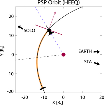
Figure 3. Polar view of the encounter 13 PSP orbit in HEEQ coordinates, where the trajectory follows a counterclockwise direction around the Sun (red) with time. The position of PSP at time t1 is shown with the spacecraft directed toward the Sun, where the purple dashed line represents the Sun-PSP line. The portion of the orbit highlighted in orange signifies the ICME event duration from time t1 to t9. The eruption axis of the event is shown by the black dashed line, aligned with active region AR 13102. The shock plane and normal are shown with a red line segment and arrow, respectively. In addition, the orbital positions of SOLO, STA, and the Earth are indicated by black arrows.
Download figure:
Standard image High-resolution imageTable 2. Upstream and Downstream Plasma Conditions at Time t1
| Plasma Parameter | Upstream | Downstream |
|---|---|---|
| vR (km s−1) | 333 ± 10 | 455 ± 16 |
| vT (km s−1) | 8 ± 17 | −358 ± 46 |
| vN (km s−1) | 60 ± 32 | 251 ± 41 |
| BR (nT) | −602 ± 20 | −1349 ± 43 |
| BT (nT) | 86 ± 59 | 142 ± 196 |
| BN (nT) | 102 ± 75 | 317 ± 222 |
| ωp (km s−1) | 113 ± 4 | 294 ± 13 |
| ne (cm−3) | 1962 ± 74 | 3989 ± 60 |
Note. Upstream and downstream conditions from the leading discontinuity at time t1 for the RTN velocity v RTN, RTN magnetic field B RTN, proton scalar thermal speed ωp , and electron number density ne . The uncertainties are based on the ensemble of outcomes from sampling the upstream and downstream conditions.
Download table as: ASCIITypeset image
2.4. ICME Sheath and Flank
Before encountering the region influenced by the ICME at time t1, the electron strahl is directed 180° from the magnetic field direction (Figures 2(g–h)). We can examine the evolution of the ePADs to study the magnetic topology of the event. After the discontinuity at t1, the electron distributions evolve differently depending on energy, shown in Figure 4 from 17:25 to 17:45 UTC. Each panel displays a different energy between ∼200 eV and 2 keV, spanning most of the instrumental range. The ePADs with energies exceeding 750 eV exhibit a strong peak near 90°, most likely associated with the ICME shock. As the energy decreases, the peak in the distribution slowly shifts toward higher pitch angles. Eventually, the ePADs appear diffuse with no strong indication of bidirectional electrons. However, ePADs below 300 eV retain a distinct strahl flowing antiparallel to the magnetic field. The duration of the 90° ePADs is dependent on energy but primarily concludes around time t2a (17:33:04 UTC).

Figure 4. Time series from 17:25 to 17:45 UTC on 2022 September 5, showing the (a) RTN magnetic field vector with magnitude (black). The normalized ePADs are shown for energies (b) 2072 eV, (c) 1401 eV, (d) 947 eV, (e) 779 eV, (f) 640 eV, (g) 526 eV, (h) 433 eV, and (i) 241 eV. The time intervals t1 and t2a are designated by the vertical dashed lines. The ePADs above 750 eV exhibit a strong peak near 90°, while electrons below 300 eV show a distinct strahl flowing antiparallel to the magnetic field.
Download figure:
Standard image High-resolution imageWhile the strahl measured below 300 eV by SPAN-E are predominantly unidirectional following time t2a
, the ePADs above 300 eV remain diffuse. A small rotation in θB
of about 50° is centered around this t2a
from 17:32:33 to 17:34:37 UTC (Figure 2(d)). After this time, the magnitude of the fluctuations in
B
diminishes, suggesting the spacecraft exits the ICME sheath region. Furthermore, v, Tp
, and B reach maximum values a few minutes after t2a
of approximately 1375 km s−1, 2300 eV, and 1640 nT, before gradually decreasing in Figure 2. Typical evidence of an MC is identified at time t2b
(18:02:26 UTC), when  and the fluctuations in
B
diminish further. At time t3a
(19:08:46 UTC), SPAN-E observes dominantly bidirectional electrons for energies above 300 eV, accompanied by a period of high density (∼104 cm−3). This interval of bidirectionality is one of the clearest examples ever observed by PSP during an encounter. This interval is strongly suggestive of closed magnetic field lines driven out into interplanetary space by the ICME. Subsequent to time t3a
, the alpha particles return to the energy range measured by SPAN-I with na
/np
> 8% (Figure 1(d)). This interval of high na
/np
is not typical of solar wind plasma, and may indicate the ICME flank. Furthermore, PSP detects two rotations in θB
of about 40° starting at 19:15:30 UTC, with a period of ∼20 minutes. FIELDS also observes a small rotation in ϕB
of more than 30° over 5 minutes, centered around 19:18:30 UTC. Following time t3b
(19:49:23 UTC), the plasma density drops below 1000 cm−3 and
and the fluctuations in
B
diminish further. At time t3a
(19:08:46 UTC), SPAN-E observes dominantly bidirectional electrons for energies above 300 eV, accompanied by a period of high density (∼104 cm−3). This interval of bidirectionality is one of the clearest examples ever observed by PSP during an encounter. This interval is strongly suggestive of closed magnetic field lines driven out into interplanetary space by the ICME. Subsequent to time t3a
, the alpha particles return to the energy range measured by SPAN-I with na
/np
> 8% (Figure 1(d)). This interval of high na
/np
is not typical of solar wind plasma, and may indicate the ICME flank. Furthermore, PSP detects two rotations in θB
of about 40° starting at 19:15:30 UTC, with a period of ∼20 minutes. FIELDS also observes a small rotation in ϕB
of more than 30° over 5 minutes, centered around 19:18:30 UTC. Following time t3b
(19:49:23 UTC), the plasma density drops below 1000 cm−3 and  . This interval is also marked by diffuse ePADs, suggesting PSP no longer observes closed magnetic field lines.
The low-density period continues until time t4a
(20:09:05 UTC), when n abruptly increases to ∼7300 cm−3, shown in Figure 5. The radial component of
B
intermittently flips polarity between times t4a
and t4b
(21:19:06 UTC), along with the dominant direction of the strahl. This indicates the first magnetic inversion line that PSP travels through during the event. Within this interval, the values of MA
and
β
p
simultaneously increase to ∼3 and ∼1, respectively. In addition, PSP measures sharp rotation in θB
of more than 50°. The rotation in ϕB
is instead more gradual over time, rotating 180° until time t5a
(22-09-06/01:14:17 UTC). The sign of BR
is consistently positive after time t4b
, when the strahl is predominantly flowing parallel to the magnetic field direction, suggesting PSP is no longer grazing the inversion line. Moreover,  is observed for a brief interval of ∼22 minutes after t4b
. At time t5a
, the strahl distribution becomes more consistent and unidirectional, indicating open field lines. PSP observes v and Tp
to decline gradually from ∼850 to 330 km s−1 and from ∼400 to 40 eV, respectively. This change is paired with MA
and β decreasing to ∼1 and ∼0.1, respectively. This shift toward typical solar wind conditions may indicate that PSP is no longer traveling through ICME plasma. As PSP exits this region, the spacecraft observes a θB
rotation from −75° to 0° over more than one hour. After time t5b
(03:26:00 UTC), the observed plasma parameters presented in Figure 5 become less variable.
is observed for a brief interval of ∼22 minutes after t4b
. At time t5a
, the strahl distribution becomes more consistent and unidirectional, indicating open field lines. PSP observes v and Tp
to decline gradually from ∼850 to 330 km s−1 and from ∼400 to 40 eV, respectively. This change is paired with MA
and β decreasing to ∼1 and ∼0.1, respectively. This shift toward typical solar wind conditions may indicate that PSP is no longer traveling through ICME plasma. As PSP exits this region, the spacecraft observes a θB
rotation from −75° to 0° over more than one hour. After time t5b
(03:26:00 UTC), the observed plasma parameters presented in Figure 5 become less variable.
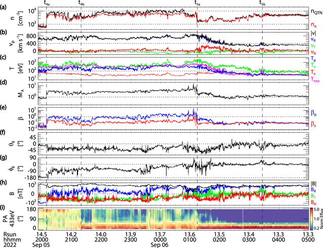
Figure 5. Time series from 22-09-05/19:52 to 22-09-06/05:00 UTC as observed by PSP. (a) QTN (black) and core (red) electron density, (b) RTN proton velocity with magnitude (black), (c) proton (blue), alpha particle (green), core electron (red), and expected proton (magenta) temperature, (d) Alfvén Mach number, (e) proton (blue) and electron (red) plasma β, (f) magnetic field elevation angle, (g) magnetic field azimuthal angle, (h) RTN magnetic field with magnitude (black), and (i) normalized ePADs at 433 eV. The magnetic field angles have been smoothed using a moving average of 5.5 minutes. The heliocentric distance of PSP in RS is shown at the bottom along the time axis. The vertical dashed lines represent different time intervals, corresponding to the intervals in Table 1, from t4a to t5b .
Download figure:
Standard image High-resolution image2.5. ICME Wake
After time t6 (08:39:49 UTC), the ePADs diffuse across the pitch angles while maintaining a preference toward 0°, illustrated in Figure 6. In addition, the values of ne , MA , and plasma β suddenly decrease below 1000 cm−3, 0.02, and 0.4, respectively. The alpha particle temperature Ta abruptly increases above 400 eV, while na /np drops below 4%. This interval is characterized by a sub-Alfvénic region behind the ICME unique to the first half of the event.
Figure 6. Time series from 22-09-06/08:00 to 22-09-07/15:00 UTC as observed by PSP. (a) QTN (black) and core (red) electron density, (b) RTN proton velocity with magnitude (black), (c) proton (blue), alpha particle (green), core electron (red), and expected proton (magenta) temperature, (d) alpha particle to proton number density ratio, (e) Alfvén Mach number, (f) proton (blue) and electron (red) plasma β, (g) RTN magnetic field with magnitude (black), and (i) normalized ePADs at 433 eV. The heliocentric distance of PSP in RS is shown at the bottom along the time axis. The vertical dashed lines represent different time intervals, corresponding to the intervals in Table 1, from t6 to t9.
Download figure:
Standard image High-resolution imageBetween times t7a (17:27:28 UTC) and t7b (17:40:00 UTC) shown in Figure 7, both MA and βp become greater than 1, while v and Tp increase above 600 km s−1 and 700 eV, respectively. At the beginning of this interval, ϕB rotates from 0° to 180° in <2 minutes, while θB fluctuates between −40° and 40° (not shown). The spacecraft passes through a second magnetic inversion line during this period as evidenced by the strahl polarity changing from 0° to 180°. The plasma conditions before t7a and after t7b are highly asymmetric, most likely attributed to different sides of a current sheet (CS). A reconnection exhaust is observed during this crossing, characterized by proton flow speed (Figure 7(b)) and temperature (Figure 7(c)) enhancements, and a significant drop in the magnetic field strength (Figure 7(g)).

Figure 7. Time series from 22-09-06/17:20 to 22-09-06/17:50 UTC as observed by PSP during the second magnetic inversion line crossing. (a) QTN (black) and core (red) electron density, (b) RTN proton velocity with magnitude (black), (c) proton (blue), alpha particle (green), core electron (red), and expected proton (magenta) temperature, (d) alpha particle to proton number density ratio, (e) Alfvén Mach number, (f) proton (blue) and electron (red) plasma β, (g) RTN magnetic field with magnitude (black), and (i) normalized ePADs at 433 eV. The heliocentric distance of PSP in RS is shown at the bottom along the time axis. The vertical dashed lines represent the t7a and t7b time intervals, corresponding to Table 1.
Download figure:
Standard image High-resolution imageAfter time t7b , n, and v decrease below 100 cm−3 and 300 km s−1, respectively. This interval is followed by a dominantly sub-Alfvénic region of space with MA ∼ 0.1. In addition, SPAN-I observes a considerable alpha particle depletion that does not appear to be an instrumental artifact (not shown). This low-density region may be a result of PSP traveling through the rear region of the ICME. After 17:48:30 UTC, v and Tp decrease below 150 km s−1 and 100 eV respectively. These conditions persist for more than 12 hr until time t8 (2022 September 7 at 06:11:28 UTC), when n and MA begin to rise, while na /np slightly decreases to 0.01. The increase in ne may indicate that ambient solar wind is flowing through the region behind the ICME. Eventually, at time t9 (11:30:16 UTC), PSP exits the sub-Alfvénic region and observes solar wind parameters similar to pre-event conditions, indicating the end of the event.
3. CME Reconstruction From Remote Sensing
Besides in situ instrumentation, PSP includes The Wide-field Imager for Solar PRobe Plus (WISPR; Vourlidas et al. 2016). WISPR is situated on the ram side of PSP and is comprised of two telescopes with a combined 95° radial by 58° transverse FOV and spatial resolution of 6 4. The range of the inner (WISPR-I) and outer (WISPR-O) telescopes span from 13
 5 to 53° and 505 to 1085, respectively. A snapshot of the combined WISPR FOV on 2022 September 5 at 17:30 UT is shown in Figure 8. This image has been processed via the L3 Algorithm developed by the WISPR team and detailed in the Appendix of Liewer et al. (2023). High particle density is associated with brighter regions in the white-light image. WISPR, along with other remote-sensing instruments discussed below, observes the beginning of the CME eruption on 2022 September 5 at ∼16:10 UT. At time t1 when PSP detects a fast-forward shock, WISPR images a clear, high-density spherical front. The leading edge observed by WISPR continues to propagate beyond PSP toward larger heliocentric longitudinal values after t1.
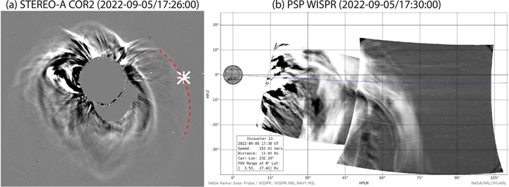
Figure 8. Remote-sensing observations of the CME on 2022 September 5 near time t1 when PSP encountered a fast-forward shock. (a) Running difference COR2 image from STA at 17:26 UT, where the location of PSP is represented by the white asterisk. An expanding front observed by COR2 is outlined by a red dashed curve. (b) Combined FOV of WISPR-I (left) and WISPR-O (right) at 17:30 UT, processed using the L3 algorithm and overlaid on a grid of heliocentric longitude and latitude. The Sun is shown to scale at the origin, with an overlaid Carrington map from the Helioseismic and Magnetic Imager onboard the Solar Dynamics Observatory (SDO/HMI). The orbital plane of PSP is represented by the blue line. The corresponding spacecraft speed, distance from the Sun, Carrington longitude, and FOV range at 0° latitude for this time are reported near the bottom left.
Download figure:
Standard image High-resolution imageAdditional imagers on board other spacecraft observed the ICME event, such as the Sun Earth Connection Coronal and Heliospheric Investigation (SECCHI; Howard et al. 2008) instrument suite on STA. SECCHI comprises five telescopes that cover a wide FOV from the Sun to interplanetary space. One of these telescopes, called COR2, is a visible light Lyot coronagraph with an FOV extent of 2–15 RS from the Sun. Figure 8(a) displays a running difference image from the COR2 telescope on 2022 September 5 at 17:26 UT. STA observes a wide-angled CME halo event during this time. As the expelled material expands with time, it appears to envelop the Sun. This suggests that at least a portion of the plasma propagates along the Sun–observer line. Both the COR2 and WISPR snapshots in Figure 8 represent the images observed nearest to time t1, when PSP encounters an ICME shock. During this time, COR2 observes a front, outlined by a red dashed curve in Figure 8(a), that is considered a shock candidate. While this front appears to intercept PSP, we note that the coronagraph observations represent line-of-sight integrated emission, and are not sufficient to determine if this front reaches PSP. Therefore, it is possible that PSP could be behind or in front of the CME shock.
To better evaluate the relative position between the ICME and PSP, we reconstruct the CME using forward modeling, as in C. R. Braga et al. (2023, in preparation). As CMEs are optically thin, coronagraphs only measure the integrated brightness over many layers along the line of sight. While these observations provide a limited perspective, we can implement CME reconstruction to improve our overall understanding. The forward modeling from C. R. Braga et al. (2023, in preparation) implements a graduated cylindrical shell (GCS) model (Thernisien et al. 2006; Thernisien 2011; Braga et al. 2022) of a flux rope structure. This empirical model is created from two conical legs connected to a curved tubular front with a cross section that increases with the distance from the solar surface. This shape is sometimes referred to as a "hollow croissant." The model is governed by three positional parameters (Stonyhurst latitude θ, Stonyhurst longitude ϕ, and tilt angle of the source region neutral line γ), two angular widths (angular width 2αw
between the legs and half-angle δ of the conical leg), and the CME height h. The half-angle δ is sometimes rewritten in terms of the aspect ratio  , which sets the expansion rate versus the CME height. In addition, we assume that the CME expands self-similarly, i.e., all model parameters are kept constant, except the height h. These free parameters are determined based on observations from the SECCHI and WISPR instruments, along with the Large Angle Spectroscopic Coronagraph (LASCO; Brueckner et al. 1995) on board the Solar and Heliospheric Observatory (SOHO; Domingo et al. 1995).
To reach an agreement with coronagraph observations, this event is modeled by two separate CMEs, denoted as the primary and secondary portions of the CME event. Figure 9 shows the primary CME (CME1) and secondary CME (CME2) at various stages of their expansion. CME1 erupted on the backside of the Sun with respect to Earth, propagating away from the planet. The model parameters for CME1 are θ = 168°, ϕ = −20°, γ = 66°, αw = 45°, and δ = 43°. Figure 9(a–b) shows CME1 (blue) at the time that PSP observes a fast-forward shock (t1), with a height of h = 14 RS . The CME is projected in HEEQ coordinates for both the polar and equatorial planes. The dark blue outline represents the cross section of the structure with the PSP orbital plane. The spacecraft is predicted to enter the flank of CME1 for a brief period of time from ∼19:40 UT to 20:20 UT, skimming the outer edge of the tubular front depicted in Figure 9(c–d). About 02:30 UT on September 6, PSP travels through a leg of CME1, where the height has expanded to h = 104 RS , shown in Figure 9(e–f). The parameters for CME2 are θ = 241°, ϕ = 5°, γ = 0°, αw = 20°, and δ = 23°. This CME is modeled to propagate quasi-perpendicular to the Sun–Earth line. The spacecraft enters CME2 on September 6 around 16:40 UT, when h = 202 RS , shown in Figure 9(g–h). This time closely corresponds to t7 when PSP crosses the second magnetic inversion line.
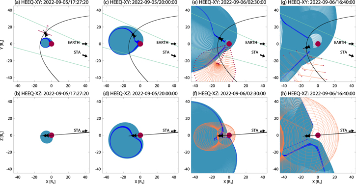
Figure 9. Encounter 13 PSP orbit in HEEQ coordinates, where the trajectory follows a counterclockwise motion around the Sun (red, not to scale) with time. The CME1 (blue region) model at time 22-09-05/17:27:20 UT, when PSP observes a fast-forward shock, is shown in the (a) XY plane (solar equatorial plane) and (b) XZ plane. The dark blue outline corresponds to the CME cross section within the orbital plane of PSP. The shock plane and normal are represented by a red line segment and arrow, respectively. At time 22-09-05/20:00 UT when PSP briefly enters the flank, CME1 is illustrated in the (c) XY plane and (d) XZ plane. Both CME1 and CME2 (orange region) at time 22-09-06/02:30 UT, when PSP enters the leg of CME1, are shown in the (e) XY plane and (f) XZ plane. The dark red outline along the wire frame of CME2 corresponds to the cross-sectional area within the orbital plane of PSP. At time 22-09-06/16:40 UT, when PSP passes the second magnetic inversion line, CME1 and CME2 are modeled in the (a) XY plane and (b) XZ plane. In addition, the orbital position of STA and Earth are depicted by black arrows, with the coronagraph COR2 FOV extent portrayed by two green lines in the solar equatorial plane.
Download figure:
Standard image High-resolution imageIt is important to note that the CME model will only reconstruct the large-scale morphology, and not necessarily the small-scale structure observed by PSP. In addition, self-similar propagation may not hold for the entire duration of this event. This event is only observable to COR2 and LASCO C3 between ∼16:30 and ∼18:30 UT. After this period, the CME reaches the outer edge of these coronagraphs and we do not have sufficient observational constraints to evaluate whether self-similarity is maintained. Moreover, the CME may experience some deflection, distortion, or rotation as it propagates from the Sun. Even with three observational points of view, we expect an error of CME propagation up to 1–2 hr (McComas et al. 2023). A more detailed description of the CME models and their agreement with coronagraph observations can be found in C. R. Braga et al. (2023, in preparation).
We now have a model that is constrained by remote-sensing estimates and geometrical assumptions for the expansion rate of the CME. To compare the model with in situ data, Figure 10 shows a snapshot of the event at 19:10 UT on 2022 September 5 near time t3a . This time is denoted by closed field lines possibly related to the flank of the structure. Due to the limited cadence of the imaging observations, the closest COR2 image to this time is 19:11 UT, illustrated in Figure 10(a). Similarly, Figure 10(b) shows the WISPR image at 19:07 UT, observed near time t3a . Figure 10(c) portrays the PSP orbital position at 19:10 UT, along with CME1. Finally, a subset of the in situ data is shown in Figure 10(d), spanning from 15:10 to 23:10 UT. The black vertical line is centered at 19:10 UT indicating the time of the current observation. An animation of this figure is available, spanning from 22-09-05/13:00 to 22-09-07/16:00 UT.
Figure 10. Combination of in situ data, remote-sensing observations, and CME modeling for the ICME on 2022 September 5 near time t3a , when PSP observes closed magnetic field lines based on bidirectional electrons. (a) Running difference COR2 image from STA at 19:11 UT, where the location of PSP is represented by the white asterisk. (b) The combined WISPR FOV at 19:07 UT, overlaid on a grid of heliocentric longitude and latitude, with an SDO/HMI Carrington map overlaid on a scale representation of the Sun. (c) PSP orbital trajectory in HEEQ coordinates at 19:10 UT, with CME1 in blue. The orbital locations of SOLO, STA, and the Earth are shown by black arrows. (d) In situ measurements observed by PSP. From top to bottom, the electron density from QTN (blue) and SPAN-E (red), solar wind velocity spectra from SPAN-I, RTN magnetic field vector with magnitude (black), and normalized ePADs measured at 433 eV. The time series is between 15:10 and 23:10 UT, with a vertical black bar indicating the time 19:10 UT. An animation of this figure is available in the online Journal, spanning from 22-09-05/16:00 to 22-09-07/12:00 UT, syncing the different cadence rates of the coronagraph imaging, in situ measurements, and CME modeling. A high-resolution version of the animation is provided by Romeo (2023).
(An animation of this figure is available.)
Download figure:
Video Standard image High-resolution imageBased on the animation from Figure 10, COR2 and WISPR begin to observe a perturbation in the white-light images around 16:10 UT. According to the GCS model, CME1 erupts around 16:10 UT on 2022 September 5, while CME2 is modeled to erupt around 20:30 UT. The in situ instruments on board PSP observe CME perturbed plasma after t1, more than an hour after the eruption. By the end of the event at time t9, both in situ and remote-sensing measurements (shown in the animation) return to pre-CME conditions.
4. Large-scale Reorganization of the Coronal Field
The in situ data observed by PSP and SOLO can be used in combination with Potential Field Source Surface (PFSS) models (Altschuler & Newkirk 1969; Schatten et al. 1969) to investigate the effect of the eruption on the large-scale configuration of the solar corona. While the CME reconstruction detailed in Section 3 models the large-scale morphology of the density structure carried by the CME, it does not constrain the magnetic structure and how it interacts with the coronal field, nor inform about the solar origin of the event. We follow the framework described in Badman et al. (2020) to project in situ magnetic polarity measurements taken by PSP and SOLO (Horbury et al. 2020) down to spatial coordinates in the outer corona before and after the CME eruption. We compare these measurements with a PFSS extrapolated model of the HCS before and after the eruption, examining the global magnetic topology, and how it relates to the source active region of the CME as seen in photospheric magnetograms.
In this study, we implement Air Force Data Assimilative Flux Transport (ADAPT; Arge et al. 2010) magnetograms modeled from Global Oscillation Network Group (GONG; Harvey et al. 1996) observations. Referred to as ADAPT-GONG magnetograms, these synoptic maps provide the lower boundary condition of the magnetic field at the surface of the photosphere. The PFSS model assumes a magnetostatic corona with zero current between the photosphere and an equipotential source surface region with a radius of RSS = 2.5 RS . At the source surface, the magnetic field lines are assumed to be radial, with solar wind plasma flowing away from the Sun along open field lines. With these assumptions, the coronal field is represented as a scalar potential allowing the PFSS model to generate the three-dimensional magnetic field structure within the modeling domain.
Figure 11 shows the ADAPT-GONG magnetograms in Carrington coordinates observed roughly one week before and after the CME event. The red and blue shadings on the synoptic maps indicate positive and negative radial photospheric magnetic fields, respectively. The nominal HCS is calculated from the PFSS model and shown in each magnetogram as a black curve. To connect these results with PSP in situ measurements above 13 RS from the Sun, the spacecraft orbit is ballistically propagated toward the source surface (Nolte & Roelof 1973). For any given point in space, the position of PSP can be connected back toward the Sun along its corresponding Parker spiral field line based on the measured solar wind speed. The orbital trajectories for PSP and SOLO are ballistically mapped down to the source surface in Figure 11, where the black and white squares indicate the initial and final positions of each orbit, respectively. The orbits are colorized according to the measured polarity of the magnetic field at each spacecraft. The orbits span about one month for each magnetogram and include a few data gaps in the magnetic field. By including the magnetic field observed by SOLO, we can compare the polarity measured by PSP before and after the event.
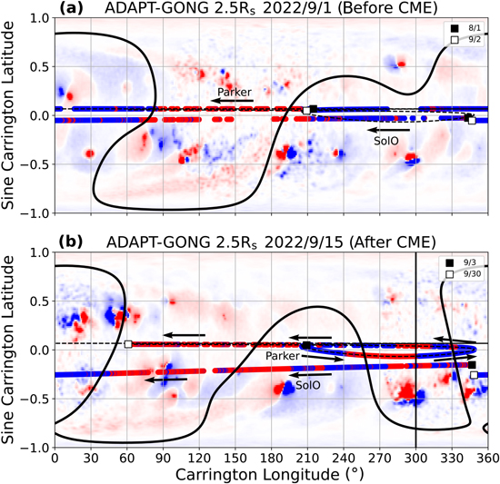
Figure 11. ADAPT-GONG magnetograms observed on (a) 2022 September 1, prior to the CME eruption, and (b) 2022 September 15, after the CME and rotation of the source active region into view. The red and blue map shadings indicate positive and negative radial photospheric magnetic fields, respectively. The black curve represents the nominal HCS obtained through a potential field source surface extrapolation for a given magnetogram. The trajectories of PSP and SOLO are ballistically mapped down to the same altitude as the HCS and colorized according to the measured polarity in space. The black and white squares indicate the initial and final positions of each orbit, respectively, with arrows depicting the orbital direction. The in situ data in panel (a) show a two-sector structure of the magnetic field over the course of the Carrington rotation prior to the CME. Four polarity sectors emerge after the CME, where one of the positive sectors is aligned with the location of the source active region (AR 13102) near  , indicating a large-scale reconfiguration of the HCS.
Download figure:
Standard image High-resolution imageIn Figure 11(a), the magnetogram was computed with observations during a full Carrington rotation until 2022 September 1, prior to the ICME event. The modeled HCS structure agrees well with the polarity flip measured by PSP and SOLO. Between August 01 and September 02, both PSP and SOLO traverse the entire longitudinal range of the Sun. The magnetic field has a two-sector structure over the course of the Carrington rotation prior to the ICME. We define a sector as a region of a dominant polarity of the radial field, bounded by the HCS and the solar equator. After the event, the magnetic field substantially changes globally, shown in Figure 11(b) with four sectors. A new sector of positive polarity emerged above 180° in Carrington longitude that is aligned with an active region (AR 13102) at  . The vertical black line in Figure 11(b) depicts the location of PSP at time t7a
when the spacecraft crosses the second magnetic inversion line. This would suggest a strong coronal reconfiguration occurred during the CME event, and a new large-scale warp in the HCS was introduced by the CME advecting the neutral line of the source active region out into space.
. The vertical black line in Figure 11(b) depicts the location of PSP at time t7a
when the spacecraft crosses the second magnetic inversion line. This would suggest a strong coronal reconfiguration occurred during the CME event, and a new large-scale warp in the HCS was introduced by the CME advecting the neutral line of the source active region out into space.
5. Discussion
Numerous studies have compared remote-sensing and in situ measurements of ICMEs near Earth (e.g., Möstl et al. 2009; Rouillard et al. 2010; Bothmer & Mrotzek 2017). PSP provides a new viewpoint near the Sun, which can help constrain ICME structure and dynamics earlier in its evolution. The spacecraft has observed a few ICMEs earlier in its mission (e.g., Lario et al. 2020; Nieves-Chinchilla et al. 2022; McComas et al. 2023), but we expect to observe more events as the Sun approaches solar maximum. This specific event is unique in that PSP traversed through the flank and wake of the structure for nearly two days (a novel situation enabled by the uniquely low perihelion and high prograde angular velocity of PSP), resulting in an interesting combination of in situ measurements which are difficult to fully explain with simple modeling approaches. Based on the animation of Figure 10, some aspects of the event clearly match the in situ measurements, remote-sensing observations, and CME modeling. Both the coronagraphs and modeling report an eruption time of the event around 16:10 UT. COR2 and WISPR also observe a large quasi-spherical front passing PSP near time t1, when the spacecraft was ∼15.05 RS from the Sun. After performing a shock geometry analysis using SPAN and FIELDS data, we find a nonradial shock normal near PSP at time t1. As PSP is closer to the flank than the apex of the ICME, we would not expect the shock normal to be radial. Between times t1 and t2a , the magnetic field fluctuations increase due to the turbulence of the sheath region. We also observe 90° ePADs for energies primarily above 750 eV. These electrons may be heated due to adiabatic compression from the shock (Manchester et al. 2012). Liu et al. (2022) have suggested the enhancement of perpendicular suprathermal electrons from interplanetary shocks could be attributed to whistler heat flux instabilities through pitch-angle scattering along with normal betatron acceleration of electrons. Furthermore, PSP measures enhanced wave activity in the AC spectra (not shown) from FIELDS during this interval. Thus, the period from t1 to t2a is denoted as the ICME sheath region, characterized by a transition to more turbulent magnetic field measurements.
After the sheath region, PSP observes some classical signatures of MCs, such as magnetic field enhancements, small rotations, low plasma β, and low Tp . However, not all of these features are measured simultaneously, or persist for the same duration. Moreover, we do not see a large rotation in the magnetic field typically associated with flux ropes. One reason that PSP does not observe a MC could be due to the spacecraft's distance from the center of the ICME (Cane et al. 1997; Kilpua et al. 2011), or due to the gradual erosion of magnetic flux from reconnection at the MC frontal edge (Dasso et al. 2007; Ruffenach et al. 2012). This may explain why the dominant polarity prior to the first polarity inversion (negative) is inconsistent with the polarity of the leading edge of the source active region (positive). In addition, it is possible that PSP is within another region of the ICME outside of the MC. Kilpua et al. (2013) have suggested additional regions exist within an ICME, defined as the faint MC front region (between the ICME and MC front boundaries) and the broader MC rear region (between the ICME and MC tail boundaries). Statistically, front regions have been shown to have higher n, v, T, and B values than other ICME regions, while the rear region is categorized by much lower n, v, and B. The MC is recorded to have the lowest T, with higher na /np than the front region.
In addition, we do not observe bidirectional strahl during the majority of this interval, but rather diffuse ePADs. One possible explanation could be that the magnetic field lines have reconnected in the CME legs with open field lines (Gosling et al. 1995), or that electron flows are typically stronger in the direction that corresponds to the local flow of the nearest footpoint (Pilipp et al. 1987). The only interval to show strong bidirectionality is from t3a to t3b and corresponds to PSP slightly grazing the flank of the CME1 model within an error of 1–2 hr. The small rotations in B , low plasma β, and low Tp may indicate the presence of an MC at time t3a , but the measured density is much lower before this interval. Eventually, PSP crosses a magnetic inversion line at time t4a , entering a region of more turbulent and dense plasma. This interval may be associated with turbulence seen in the flank and wake regions of ICMEs (Fan et al. 2018). After t5a , v and T decrease until the plasma is observed to return to typical values for ambient solar wind at these heliocentric distances. The spacecraft may be within a region where new solar wind has begun to fill the ICME wake. However, PSP appears to observe a new transient with a sub-Alfvénic flow at time t6. PSP crosses a second magnetic inversion line at time t7a . The two portions of the ICME may be separated by this current sheet, where one side is observed to be highly sub-Alfvénic. However, one must be careful when interpreting CME2 as it does not have an associated active source region based on these observations. This could suggest that CME1 and CME2 are produced by the same active region, erupting at different times. CME2 could also be a stealth CME, which is an eruption with no low coronal signatures (LCSs) to identify a source region (Robbrecht et al. 2009; Ma et al. 2010). However, Alzate & Morgan (2017) has associated these type of events with limitations regarding remote-sensing observations and image processing. The LCSs related to stealth CMEs may form higher in the corona or low-density regions (Alzate & Morgan 2017). Observations from SOLO may provide more insight into CME2 and any associated LCSs as the spacecraft observed the backside of the Sun during the event (Long et al. 2023).
Figure 12(a) illustrates a simple interpretation of the event informed by the ADAPT-GONG magnetograms, PFSS model, and PSP in situ data. We consider a single CME, where PSP travels along a circular orbit from top to bottom in the figure. We refrain from including the orbit in the illustration as the structure evolves over the course of two days. After exiting the sheath region, PSP travels through plasma perturbed by the ICME until crossing the first ICME leg at time t4a . The magnetic field lines are directed away from the Sun in the first leg (blue region) after PSP crosses the first magnetic inversion line (purple dashed line). PSP is within the ICME leg until t7a when the spacecraft crosses another magnetic inversion line. During this interval, PSP is located directly above the active source region described in Section 4. The two polarity regions (red and blue) of AR 13102 may correspond to each leg of the ICME, indicating that PSP travels from one leg to the other at time t7. This inversion line would then correspond to the current sheet of the ICME (Lin & Forbes 2000) in its wake connected back toward the Sun. The sub-Alfvénic region after t7b may be due to an asymmetry in the flow directions during magnetic reconnection (Murphy et al. 2012). The interval between t7a and t7b could be related to a reconnection exhaust as Tp and β are higher inside this period, while ∣ B ∣ is smaller (Gosling et al. 2005; Phan et al. 2022).

Figure 12. Illustrations of (a) a single ICME model based on coronal magnetograms and in situ data, and (b) a simplified two-part ICME model based on white-light coronagraphs and in situ observations. PSP travels along a circular orbit around the Sun from top to bottom in each figure. The magnetic field lines are represented by the black curves connected to the solar surface, with arrows depicting their respective polarity. The purple dashed lines depict the magnetic inversion lines observed by PSP at times t4a and t7a . The single ICME in (a) is portrayed by the blue region, while CME1 and CME2 in (b) are shown by the blue and orange regions, respectively. The active region AR 13102 is shown on the solar surface in (a) with positive (red) and negative (blue) polarity to agree with the ADAPT-GONG magnetograms. The gray area in (b) represents the region of space outside of CME1 that PSP travels through between times t4a and t6. CME1 could be concave in three dimensions, allowing PSP to exit and re-enter the structure.
Download figure:
Standard image High-resolution imageThis illustration of the event agrees well with the magnetograms and FIELDS data but does not explain the plasma region from t2a to t4a . We would expect PSP to be within the ICME region as this interval exhibits multiple ICME in situ signatures. However, this spatial domain could be between the sheath and MC regions as PSP only travels through the flank and wake of the structure. In addition, this model does not explain the stable plasma conditions observed between t5a and t6. The ICME could have a more complex three-dimensional structure, experiencing some deformation, deflection, or rotation as it propagates from the Sun. Furthermore, this interpretation does not include a second portion of the CME, modeled to agree with white-light images. A slightly more complex interpretation with a two-part CME, as informed by the GCS modeling discussed in Section 3, is shown in Figure 12(b). The illustration portrays a deformed ICME to emphasize asymmetry within the structure. After time t2a , PSP passes through the flank of CME1 (blue region), observing numerous ICME signatures described above. At time t4a , the spacecraft exits the ICME and enters a region of space still perturbed by the eruption (gray region). This region could exist if the ICME is concave, signifying a more complex structure in three dimensions. Once the spacecraft exits the ICME, the magnetic field lines are inverted, indicating a magnetic inversion line. The perturbed plasma begins to fade away at time t5a when ambient solar wind fills the ICME wake. Plasma parameters such as n, v, and T return to expected conditions based on solar distance during this interval. PSP re-enters CME1 at t6, with field lines still oriented away from the Sun. The spacecraft enters CME2 (orange region) at time t7a , crossing another magnetic inversion line. The region after t7b is highly sub-Alfvénic and could be caused due to the expansion of CME2 within the wake of CME1 (Chané et al. 2021). This interval persists until time t9 when PSP exits the entire ICME-perturbed plasma. This model agrees with the majority of in situ signatures observed by PSP and the inclusion of CME2 from Section 3. However, Figure 12(b) does not set the second magnetic inversion line as the current sheet between the CME legs, but instead the current sheet between the two parts. If CME1 and CME2 originate from the same source region, we would expect these structures to be connected.
Both illustrations in Figure 12 offer reasonable interpretations for different aspects of this event. A more complete description would need to be more complex in three dimensions to explain the evolution of the structure as it propagates from the Sun. While not every small-scale feature of the event can be explained with the proposed models, it is clear that the HCS experienced a major reconfiguration during this period. The coronal magnetic field had a four-sector structure after the event, persisting for about two months, as evidenced independently by PSP and SOLO magnetic field data. Based on the magnetograms and PFSS model, this corresponds to time t7 when PSP is directly above the active region aligned with one of the new sectors. Thus, this CME event led to a structural change in the HCS that continued well after the eruption. CMEs release accumulated magnetic helicity and trapped energy from the corona (Low 1994). This phenomenon continues the magnetic flux transport that began from the solar interior out to interplanetary space and plays a strong role in controlling the magnetic flux budget of the Sun (Low 2001). As the Sun approaches solar maximum, the frequency of CMEs will increase and the cumulative effect of these eruptions will reconfigure the HCS more frequently until the coronal field switches polarity. Therefore, the release of magnetic helicity through CMEs could predominately control the shape of the HCS and its evolution over the solar cycle.
6. Conclusion
On 2022 September 5 at 17:27:20 UTC, PSP observed an ICME event until 2022 September 07 at 11:30:16 UTC. Numerous in situ signatures that typically correspond with ICMEs were observed, such as bidirectional strahl, low Tp , low β, na /np > 8%, directional discontinuities, and a fast-forward shock. The magnetic field varied from region to region with periods of enhancements, small rotations, and turbulence. In addition, PSP measured intervals of density depletion corresponding to sub-Alfvénic regions. Besides in situ measurements, several remote-sensing observations of the event were obtained from multiple viewpoints including PSP, STA, and SOHO. Based on white-light coronagraphs, two portions of the ICME were modeled separately to fit the extent of the event.
Due to the complexity of the ICME, a simple description of the event has proven difficult when comparing in situ and remote-sensing measurements. Both proposed scenarios (see Figure 12) possess aspects that agree with PSP observations, but neither offers a complete explanation of the event. It is important to note that these interpretations only consider the large-scale structure and that the full description of the event is more complex in reality. Regardless of the necessity for a second portion of the CME, PSP still crossed two magnetic inversion lines near the Sun in the wake of an ICME. The in situ polarity data taken by crossing the ICME-perturbed longitudes, as well as PFSS extrapolations, show a global reconfiguration of the HCS after the ICME event. This would suggest these eruptions on the Sun strongly affect the HCS structure. Therefore, CMEs may have a key involvement in the evolution of the HCS throughout the solar cycle. In addition, the events described in this study may provide insight into how CMEs influence the development of young solar wind, e.g., during the extreme low-density region after t7, addressing a key science objective of the PSP mission.
To further investigate this event, future work could implement in situ plasma parameters observed by PSP into the CME forward modeling described in Section 3. The models presented in this study only considered observations from coronagraph and heliospheric imagers. The inclusion of PSP plasma data during different periods of the event may produce improved results. In addition, future studies of the ICME could incorporate measurements from the Integrated Science Investigation of the Sun (IS⊙IS; McComas et al. 2016) instrument suite. IS⊙IS is composed of two instruments that measure lower (EPI-Lo) and higher (EPI-Hi) energetic ions and electrons above the energy range of SPAN. Although EPI-Lo was not operational during this event, EPI-Hi was powered on and collected measurements of energetic particles. A comparison of SPAN, FIELDS, and EPI-Hi data would provide more information on various features of the event, such as high energy particle acceleration. In addition to PSP, SOLO observed the event on 2022 September 6 around 12:33 UT with in situ detectors. SOLO was located ∼150 RS from the Sun at the start of the event and was closer in proximity to the ICME apex than PSP. Further research with SOLO and PSP data could study CME morphology and evolution as the structure propagates farther from the Sun into interplanetary space.
Acknowledgments
The Parker Solar Probe was designed and built and is now operated by the Johns Hopkins Applied Physics Laboratory (JHU/APL) as part of NASA's Living with a Star (LWS) program (contract NNN06AA01C). Support from the LWS management and technical team has played a critical role in the success of the Parker Solar Probe mission. O.M.R is supported by NASA Future Investigators in NASA Earth and Space Science and Technology (FINESST) grant 80NSSC22K1852. C.R.B. acknowledges the support from the NASA STEREO/SECCHI (NNG17PP27I) program and NASA HGI (80NSSC23K0412) grant. J.H. is supported by NASA grant 80NSSC23K0737. J.L.V. acknowledges support from NASA PSP-GI 80NSSC23K0208 and NASA LWS 80NSSC22K1014.
The SWEAP Investigation is a multi-institution project led by the Smithsonian Astrophysical Observatory in Cambridge, Massachusetts, in collaboration with the University of Michigan, University of California, Berkeley Space Sciences Laboratory (UCB/SSL), The NASA Marshall Space Flight Center, The University of Alabama Huntsville, the Massachusetts Institute of Technology, Los Alamos National Laboratory, Draper Laboratory, JHU/APL, and NASA Goddard Space Flight Center (NASA/GSFC). The FIELDS instrument suite was designed and built and is now operated by a consortium of institutions including UCB/SSL, University of Minnesota, University of Colorado, Boulder, NASA/GSFC, CNRS/LPC2E, University of New Hampshire, University of Maryland, University of California, Los Angeles (UCLA), IFRU, Observatoire de Meudon, Imperial College, London and Queen Mary University London. SWEAP and FIELDS measurements were analyzed and visualized in the Interactive Data Language (IDL). The Wide-field Imager for Parker Solar Probe (WISPR) instrument was designed and built and is now operated by the US Naval Research Laboratory (NRL) in collaboration with JHU/APL, California Institute of Technology/Jet Propulsion Laboratory, University of Göttingen, Germany, Centre Spatial de Liège, Belgium, and Institut de Recherche en Astrophysique et Planétologie. WISPR data are available for download at https://wispr.nrl.navy.mil/.
The Sun Earth Connection Coronal and Heliospheric Investigation (SECCHI) was produced by an international consortium of the NRL (USA), Lockheed Martin Solar and Astrophysics Lab (USA), NASA/GSFC (USA), Rutherford Appleton Laboratory (UK), University of Birmingham (UK), Max Planck Institute for Solar System Research (Germany), Centre Spatial de Liège (Belgium), Institut d'Optique Theorique et Appliquée (France), and Institut d'Astrophysique Spatiale (France). STEREO/SECCHI data are available for download at https://secchi.nrl.navy.mil/. The ADAPT model development is supported by the Air Force Research Laboratory (AFRL). The input data utilized by ADAPT are obtained by the Global Oscillation Network Group (GONG) program. The PFSS models were generated using the pfsspy Python package (Stansby et al. 2020). SDO insets in Figures 8(b) and 10(b) courtesy of NASA/SDO and the AIA, EVE, and HMI science teams.
Appendix A: QTN Electron Density Algorithm
To determine the total electron density ne , we implement a new simplified heuristic algorithm based on QTN spectroscopy theory (Meyer-Vernet et al. 2017). The electron plasma frequency fp is derived from the peak with the slope of greatest ascent in a given QTN spectrum measured by a dipole antenna (see Figure 2 in Meyer-Vernet et al. 2017). By isolating the peak from other features in the spectrum, we can calculate the total electron density. To measure QTN spectra, we use the RFS from the FIELDS suite, which includes four electric antennas and a single axis of the PSP search coil magnetometer (Pulupa et al. 2017). We average the RFS LFR data from the V1–V2 and V3–V4 antenna dipole pairs, covering a frequency range of 10 kHz−1.7 MHz with 64 logarithmically spaced frequencies, providing ∼4.5% resolution. The LFR spectra are then flattened by removing a fitted quadratic function to emphasize the plasma frequency peak. We convolve the scaled spectra with a step function and apply high and low pass filters centered at 80 and 700 kHz, respectively, to highlight and smooth the plasma frequency line. Finally, we normalize the convolution for each sample by the maximum value in the spectrum.
The heuristic search algorithm is composed of three parts: an outward search, an inward search, and a comparison between the two methods. Beginning with the outward search, we identify all the local maxima for N convolved normalized spectra in a given day. A reference plasma frequency fr is selected from an ideal spectrum with only one peak (the plasma line) at time tr . From time tr , an outward heuristic search is iterated forward in time to select frequencies along the plasma line until time tN . The heuristic function implements both the local maxima values of the signal's convolution and the relative change in frequency between samples. This method assumes a smooth and continuous plasma line, which accounts for solar Type III radio bursts that contaminate the plasma line.
Given the plasma frequency at tr , we determine fp at time tr+1 by identifying each frequency bin number F (among the 64 frequency bins of the LFR spectra) with a local maxima m at time tr+1. We then compute the normalized difference in frequency bins ΔF(tr+1) between the previous plasma line frequency bin Fp (tr ) and the frequency bin for a given local maxima Fm (tr+1) as

where M is the total number of frequency bins. For each local maxima, we apply ΔF(tr+1) to a frequency heuristic function hF (ΔF), shown in Figure 13. It is important to note that we are using the frequency bin number F (1–64) and not the numerical frequency value f for the heuristic function to avoid a bias toward smaller frequencies. In addition, for each local maxima, we apply its normalized convolution value c(tr+1) to a convolution heuristic function hc (c), shown in Figure 13. An outward search heuristic function is then computed weighing both parameters as h = 0.4 hc + 0.6 hF . Based on Figure 13, the local maximum with a combination of the largest convolution value and smallest frequency bin difference is assigned the plasma frequency fp at time tr+1. This process is iterated forward in time until tN and iterated backward from time tr to t1 in a given day. Given that this algorithm identifies the plasma line from time tr toward the start and end of the day, it is referred to as an "outward search."

Figure 13. Heuristic functions h(x) for a given normalized parameter x. The frequency heuristic function hF (purple) is a function of the normalized frequency bin difference ΔF. The convolution heuristic function hc (red) is a function of the normalized convolution value of the resulting spectra.
Download figure:
Standard image High-resolution imageThe "inward search" algorithm is performed in a similar manner, except that the search begins at time t1. We select a new reference plasma frequency at the beginning of the day and iterate forward in time to tr using the same heuristic functions in Figure 13. In parallel, another search is performed from time tN to tr , iterating the process backward in time to determine the plasma line. We manually select the plasma frequency at times t1 and tN given the spectra for a complete day. This process is known as an "inward search" as both searches are iterated separately toward time tr . The purpose of bidirectional searches is to more easily determine the plasma line in cases of apparent bifurcation. In theory, the resulting frequency from either the outward search fp o or inward search fpi is the best estimate for the true plasma frequency. The final step of the algorithm compares the plasma frequencies from the two searches in an effort to determine a single value of fp at each time.
Figure 14 emphasizes the importance of comparing the outward and inward searches for the plasma line. Outside the interval between time ta
and tb
, both search algorithms agree upon the estimated plasma frequency. However, within this interval, the outward and inward searches follow different paths due to a Type III radio burst. To account for this discrepancy ( ), we compute a new modified heuristic function for each search, solely based on the relative change in frequency bins between ta
and tb
. The inward hi
and outward ho
heuristic functions are defined as
), we compute a new modified heuristic function for each search, solely based on the relative change in frequency bins between ta
and tb
. The inward hi
and outward ho
heuristic functions are defined as
where Fp o and Fpi are the plasma frequency bins determined from the outward and inward searches, respectively. The search method that results in the smallest heuristic value will be used to set fp . As ho < hi within the time interval in Figure 14, the outward search plasma frequency is selected. This is done for all time intervals that the inward and outward search algorithms do not agree.

Figure 14. Normalized convolution spectra computed from RFS LFR data on 2021 August 9, targeted on the plasma line. The plasma frequencies selected from the inward and outward searches are designated by the white and black lines, respectively. Within the interval between times ta and tb (denoted by vertical lines), the two search algorithms do not follow the same path.
Download figure:
Standard image High-resolution imageOnce the plasma frequency line is determined for a given day, we compute a geometric weighted mean frequency 〈fp
〉 between the neighboring frequency bins of the plasma line. This process is then repeated for each day to determine the total electron density with the equation  . To ensure our algorithm is performing correctly, we use the QTN electron density estimate from Moncuquet et al. (2020) for PSP encounters 1 through 10. We have determined the frequency and convolution heuristic functions shown in Figure 13 by comparing the results of Moncuquet et al. (2020). The two data sets agree within 5%–10%, which is reasonable given the 4.5% resolution of the instrument. This method offers several advantages, such as its simplicity, efficient run time of 0.5–2 minutes per day, handling of radio bursts, large fluctuations in the plasma line, and other events with low signal-to-noise ratios.
Appendix B: Empirical Solar Wind Velocity and Temperature Relationship
Based on the bulk proton speed vp
, an empirical relationship can be found with the plasma proton temperature Tp
for the ambient solar wind (Lopez 1987). However, there are instances when the measured Tp
is lower than the expected proton temperature Texp from the vp
− Tp
relation. These intervals could be associated with magnetically isolated, ejected plasma expanding faster than the ambient solar wind. They typically are preceded by interplanetary shocks, suggesting a connection to ICME shock drivers. We can expect ICMEs to follow the condition  for magnetic clouds (Richardson & Cane 1995).
Previous work has correlated vp and Tp using Wind data (Yu et al. 2014; Huang et al. 2017). However, we must determine a new empirical relationship for vp and Tp as PSP orbits much closer to the Sun than Wind. Thus, we follow a similar method from these studies to fit the expected proton temperature to the bulk proton speed using SPC and SPAN-I data for encounters 1 through 10. The data set is divided into two velocity regimes: slow solar wind (vp < 400 km s−1) and fast solar wind (vp > 400 km s−1). We perform a separate fit for each velocity regime based on the statistical formula from Lopez (1987). In addition, as the temperature scales with radial distance R from the center of the Sun, we include a power law Ra in each fit. Figure 15 displays the empirical relationship between vp and scaled Tp by Ra for both the slow and fast wind, described by
where R is in units of solar radius RS . Based on these relationships, we use vp to compute an expected proton temperature and compare Texp with the measured proton temperature from SPAN-I.
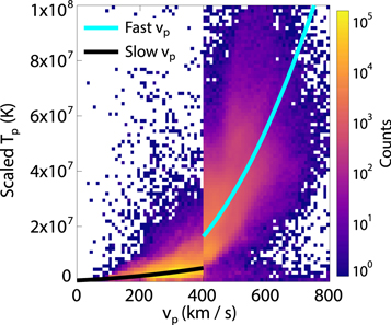
Figure 15. 2D Histogram of scaled proton temperature Tp by Ra as a function of the SW velocity vp for PSP encounters 1 through 10. The proton temperature is scaled by R0.79 in the slow solar wind and R1.10 in the fast wind. The fitted curves for the slow and fast solar winds are shown in black and cyan, respectively.
Download figure:
Standard image High-resolution image