


Abstract
Stellar coronal mass ejections (CMEs) have recently received much attention for their impacts on exoplanets and stellar evolution. Detecting prominence eruptions, the initial phase of CMEs, as the blueshifted excess component of Balmer lines is a technique to capture stellar CMEs. However, most of prominence eruptions identified thus far have been slow and less than the surface escape velocity. Therefore, whether these eruptions were developing into CMEs remained unknown. In this study, we conducted simultaneous optical photometric observations with Transiting Exoplanet Survey Satellite and optical spectroscopic observations with the 3.8 m Seimei Telescope for the RS CVn-type star V1355 Orionis that frequently produces large-scale superflares. We detected a superflare releasing 7.0 × 1035 erg. In the early stage of this flare, a blueshifted excess component of Hα extending its velocity up to 760–1690 km s−1 was observed and thought to originate from prominence eruptions. The velocity greatly exceeds the escape velocity (i.e., ∼350 km s−1), which provides important evidence that stellar prominence eruptions can develop into CMEs. Furthermore, we found that the prominence is very massive (9.5 × 10¹⁸ g < M < 1.4 × 10²¹ g). These data will clarify whether such events follow existing theories and scaling laws on solar flares and CMEs even when the energy scale far exceeds solar cases.
Export citation and abstract BibTeX RIS

Original content from this work may be used under the terms of the Creative Commons Attribution 4.0 licence. Any further distribution of this work must maintain attribution to the author(s) and the title of the work, journal citation and DOI.
1. Introduction
Solar flares are explosive phenomena wherein magnetic energy stored around sunspots is suddenly released through magnetic reconnection (e.g., Shibata & Magara 2011). Generally, a solar flare releases about 1026–1032 erg. Emission in a wide range of wavelengths from radio waves to X-rays occurs during a flare. Generally, prominence eruptions on the Sun, which are associated with flares (e.g., Sinha et al. 2019), are observed as Hα emission and Hα absorption when they erupt outside a limb and on a disk, respectively (Parenti 2014; Otsu et al. 2022). Prominence or filament eruptions can lead to coronal mass ejections (CMEs) when the prominence velocity is sufficiently large (e.g., Gopalswamy et al. 2003; Shibata & Magara 2011).
Flares are widely observed both on the Sun and stars. In the case of stars, "superflares," which release 10 times larger energies than the largest solar flares, have been confirmed (e.g., Maehara et al. 2012). Spectroscopic observations of stellar flares sometimes show "blueshifts" (or "blue asymmetries") wherein chromospheric lines during flares are not symmetric, but are enhanced only at shorter wavelengths (e.g., Houdebine et al. 1990; Gunn et al. 1994; Fuhrmeister & Schmitt 2004; Fuhrmeister et al. 2008, 2011; Vida et al. 2016; Honda et al. 2018; Vida et al. 2019; Muheki et al. 2020; Maehara et al. 2021). An excess component with a shorter wavelength than the rest line center is observed, indicating that the source is flying toward us, considering the Doppler effect. Therefore, blueshifts might suggest that an upward-moving plasma exists, such as prominence eruptions (Otsu et al. 2022) or a chromospheric temperature (cool) upflow associated with chromospheric evaporation (Tei et al. 2018). One technique to determine whether a blueshifted excess component originates from cool upflows or prominence eruptions is to estimate it based on its Doppler velocity. Typically, cool upflows have a velocity of ∼100 km s−1 in solar flares (e.g., Kennedy et al. 2015). Therefore, we can expect that blueshifts that significantly exceed this velocity originate from prominence eruptions.
Most of the blueshifts discovered thus far have been relatively slow (<500 km s−1). Almost no solid evidence exists that they originated from prominence eruptions and these eruptions triggered a CME. Namekata et al. (2022a) first discovered solid evidence of a stellar filament eruption by detecting the blueshifted absorption component of Hα. By using the length scale and the velocity of the ejected plasma, Namekata et al. (2022a) confirmed that the erupted filament very likely developed into CMEs. Further, few cases of blueshifts in flares larger than 1035 erg emerge. Generally, a positive correlation exists between the energy of solar flares and those of associated prominence eruptions (e.g., Aarnio et al. 2011; Takahashi et al. 2016). Previous blueshift examples found that events on stars generally come as an extension of this correlation (e.g., Moschou et al. 2019). Therefore, if we can detect a blueshift during a particularly large-scale superflare (>1035 erg), its kinetic energy is likely to be excessively large. This becomes reliable evidence of a stellar CME. Moreover, detection of these events can confirm whether the relation between flare energy and the size of the plasma eruption could be extended to this region.
RS CVn-type stars are magnetically active and have been observed to produce large superflares (Tsuboi et al. 2016, and references therein). Many previous studies of flares on RS CVn stars have been conducted in X-ray, whereas only a few studies have been conducted with optical spectroscopic observations. Particulaly, large-scale superflares (i.e., >1035 erg) frequently occur on RS CVn stars. In recent years, stellar CMEs have attracted much attention for their impacts on mass/angular-momentum loss and the environment of surrounding exoplanets. If existing correlations between prominence eruptions and flare energies hold for particularly large superflares (>1035 erg), prominence eruptions that accompany such flares will lead to particularly large-scale CMEs. Consequently, they will have particularly large effects on stellar evolution and exoplanets (Osten & Wolk 2015; Airapetian et al. 2020). Therefore, optical spectroscopic observations of RS CVn-type stars are important because they enable the detection of particularly large-scale superflares, which are quite infrequent to be observed on normal main-sequence stars, with only a short period of monitored observations.
In this study, optical spectroscopic observations by the 3.8 m Seimei Telescope (Kurita et al. 2020) and photometric observations by the Transiting Exoplanet Survey Satellite (TESS; Ricker et al. 2015) were simultaneously performed to V1355 Orionis, an RS CVn-type star. The observations and analysis (Section 2), results (Section 3), and discussion (Section 4) on the details of the superflare and the associated blueshift obtained through the simultaneous observations are reported in this paper.
2. Observations and Analyses
2.1. Target Star : V1355 Orionis
V1355 Orionis (=HD291095) is an RS CVn-type binary system discovered through the ROSAT WFC all-sky X-ray survey (Pounds et al. 1993; Pye et al. 1995). V1355 Orionis has been investigated by Cutispoto et al. (1995), Osten & Saar (1998), and Strassmeier (2000). These studies have shown that this binary comprises K0-2IV and G1V stars. Table 1 summarizes the basic physical parameters of the K-type subgiant star. Strassmeier (2000) reported a large flare on V1355 Orionis in 1998 April, which showed 70 times larger equivalent width of Hα than the pre-flare.
Table 1. Basic Physical Parameters of the K-type Subgiant Star of the Binary
| Spectral Type | Va | V − RC a | db | Porb c | Prot d | Re | Lf | Mg | Teff h | ve i |
|---|---|---|---|---|---|---|---|---|---|---|
| (mag) | (mag) | (pc) | (days) | (days) | (R⊙) | (L⊙) | (M⊙) | (K) | (km s−1) | |
| (1) | (2) | (3) | (4) | (5) | (6) | (7) | (8) | (9) | (10) | (11) |
| K0-2IV | 8.98 | 0.53 | 127.4 | 3.87 | 3.86 | 4.1 | 6.4 | 1.3 | 4750 | −347 |
Notes.
a The V-band magnitude and difference between the V and RC bands. b Stellar distance. c Orbital period. d Rotation period. e Radius. f Luminosity. g Mass. h Effective temperature. i Escape velocity at the surface.References. (1), (5)–(11): Strassmeier (2000), (2), (3): Cutispoto et al. (1995), and (4): Gaia Collaboration et al. (2016).
Download table as: ASCIITypeset image
2.2. Simultaneous Observations
2.2.1. Photometric Observation: TESS
TESS observed V1355 Orionis in Sector 34 for 27 days with the 2 minutes time cadence. Figure 1(a) shows the TESS light curve for this period (BJD = 2459201.7-2459227.5). Figure 1(b) shows the enlarged TESS light curve around the flare described in this paper. The quiescent radiation component during the flare is estimated by fitting a polynomial to the light curve for −500 to −10 minutes and +150 to +380 minutes from the flare start (see the sky-blue dashed line in Figure 1(b)). Figure 2(a) shows the light curve for the flare component, created by subtracting the quiescent component from the light curve of TESS during the flare. We calculated the bolometric energy of the flare from this detrended light curve following the method of Shibayama et al. (2013). See Section 3.1 for more details about caluculating the flare energy.

Figure 1. White-light light curves of V1355 Orionis observed with TESS. (a) Long-term light curve of V1355 Orionis for BJD = 2459201.7-2459227.5. The vertical axis represents the flux normalized by the median value. The vertical light-blue line and the horizontal green bars indicate the event discussed in this paper and the period of monitoring observations by Seimei telescope/KOOLS-IFU, respectively. (b) Enlarged light curve around December 19/BJD = 2459203.11297. The horizontal axis represents the time (unit of minutes) from BJD = 2459203.11297. The sky-blue dashed line shows the global trend of the stellar rotational modulation fitted for −500–10 minutes and 150–380 minutes with a polynomial equation.
Download figure:
Standard image High-resolution image
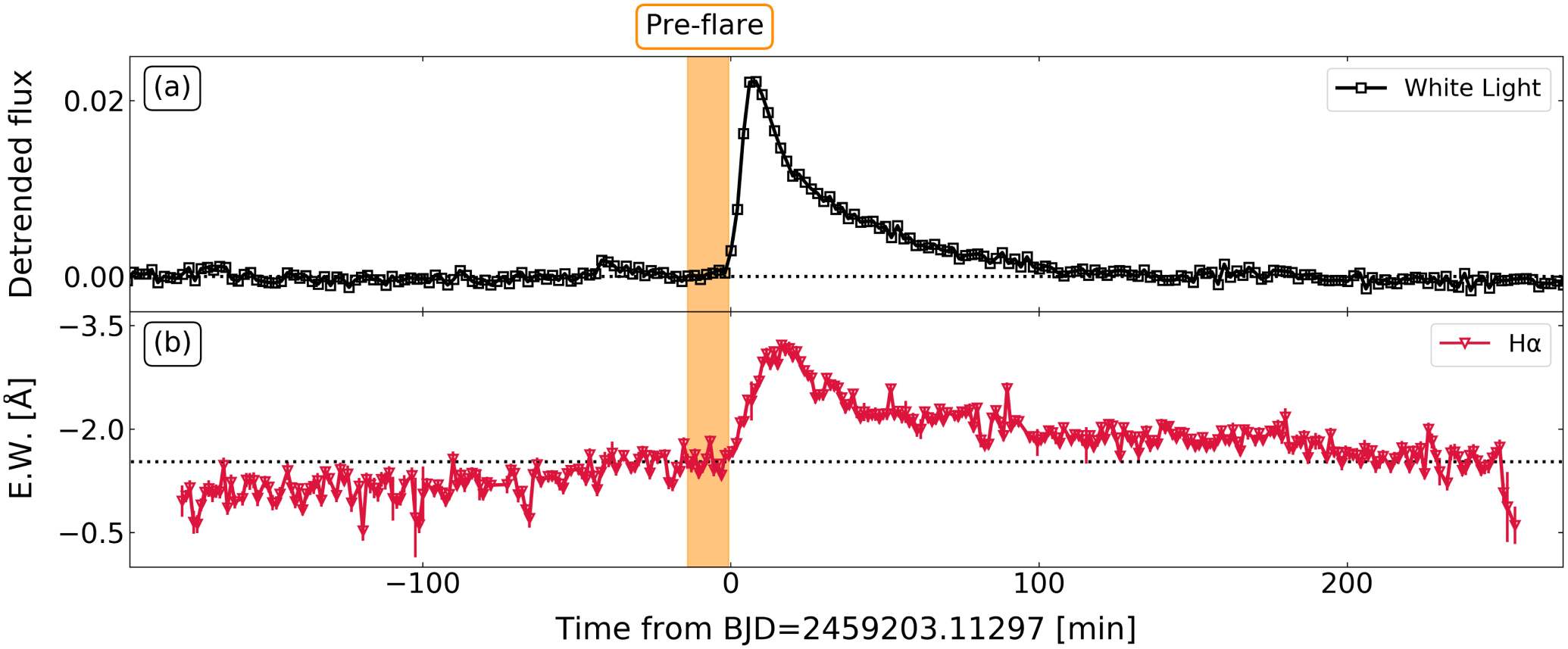
Figure 2. Light curves of V1355 Orionis during the December 19 event. (a) Detrended light curve of the TESS white light with background removed. This corresponds to the TESS normalized flux (black line in Figure 1(b)) subtracted by the rotational modulation (sky-blue line in Figure 1(b)). The black dotted line represents the zero level. The orange range indicates the time period determined as the "pre-flare" in our spectral analysis. (b) Light curve of the Hα for the same time period as in panel (a). The vertical axis shows the equivalent width of Hα. The black dotted line represents the level of background, calculated as the average of the equivalent width of the pre-flare. Note that in this light curve, the equivalent width is negative for the emission line flux.
Download figure:
Standard image High-resolution image2.2.2. Spectroscopic Observation: The Seimei Telescope
We observed V1355 Orionis using KOOLS-IFU (Kyoto Okayama Optical Low-dispersion Spectrograph with optical-fiber Integral Field Unit; Matsubayashi et al. 2019), the spectrograph on board the 3.8 m Seimei telescope (Kurita et al. 2020). KOOLS-IFU covers 5800–8000 Å with wavelength resolution R ( = λ/Δλ) of ∼2000. Therefore, it can capture the Hα line.
Observations were made over eight nights in conjunction with Sector 34 of TESS. The flare investigated in this study occurred on the first day of our observations. The detailed observation periods are indicated by the horizontal green bars in Figure 1(a). The exposure time was set to 60 s on all observation dates. The signal-to-noise ratio at the continuum around Hα line was more than 10.
Data processing was conducted in the same manner as that in Namekata et al. (2020, 2022a, 2022b) with IRAF package, Pyraf software, and the data reduction packages developed by Matsubayashi et al. (2019). Using the Hα line profile at each time frame, we investigated the time variation of the equivalent width during the flare. Figure 2(b) shows the light curve of the equivalent width of Hα. Further, the equivalent width was calculated, after normalizing Hα emission by the nearby continuum level, integrating it for 6518–6582 Å. The reason why the range of integration is asymmetric to the line center of Hα ( = 6562.8 Å) is due to the blueshifted excess component. See Section 3.2 for more information about the blueshifted excess component.
3. Results
3.1. White-light Flare Energy
As shown in Figure 2(a), the white-light flare lasted about 110 minutes. By setting the flux of Figure 2(a) to  (= luminosity of flare/luminosity of star) in the Equation (5) of Shibayama et al. (2013), we estimated the flare area
  as follows:

where λ is the wavelength, Bλ
is the Planck function, Rλ
is the TESS response function (Ricker et al. 2015), and Ti
is the effective temperature of the K- and G-type stars of the binary (4750 K and 5780 K, respectively; Strassmeier 2000). Further,  represents a flare temperature of 10,000 K (Mochnacki & Zirin 1980; Hawley & Fisher 1992), and Ri
is the radius of the K- and G-type stars of the binary (4.1R⊙ and 1.0R⊙, respectively; Strassmeier 2000). Assuming that the flare can be approximated by blackbody radiation with a temperature of
represents a flare temperature of 10,000 K (Mochnacki & Zirin 1980; Hawley & Fisher 1992), and Ri
is the radius of the K- and G-type stars of the binary (4.1R⊙ and 1.0R⊙, respectively; Strassmeier 2000). Assuming that the flare can be approximated by blackbody radiation with a temperature of  , flare luminosity
  is
is

where σSB is the Stefan–Boltzmann constant. Finally, by integrating  with the duration of the white-light flare (∼110 minutes), the bolometric flare energy Ebol is

Given that the K-type star is more magnetically active and the bolometric flare energy is very large, we consider this flare to have occurred on the K-type star of the binary.
3.2. Hα Line Profile during the Flare
Our spectroscopic observation revealed that a remarkable blueshifted excess component exists in the Hα emission line for ∼30 minutes after the start of the flare. Figure 3(a) shows the spectra during the time when the blueshifted excess component was observed during the flare. We estimated the spectrum of the quiescent component, denoted by red spectrum in Figure 3(a), by combining the spectra from 15 minutes before the flare start ("pre-flare"). Figure 3(b) shows the spectrum of the flare emission component, which were obtained by obtaining the difference between the spectrum at each time and the pre-flare spectrum. A particularly large blueshifted excess component was observed in the pre-flare subtracted spectrum, especially 5–18 minutes, extending over −1000 km s−1. Figure 4(d) presents a color map showing the time variation of the blueshifted excess component in the pre-flare subtracted spectrum. The blueshifted excess component was fast over the time period when white light and Hα reach their peak.

Figure 3. Time variation of the Hα spectrum in the early stages of the flare. (a) Line profile of Hα emission. Each spectrum is a composite of three (= 3 minutes) spectra. The bottom and top axes are the wavelength and Doppler velocity from the line center, respectively. The intensity of each spectrum is normalized by the continuum. The vertical dotted and horizontal dashed lines represent the line center of Hα and the continuum level for each spectrum, respectively. The spectrum at each time is vertically shifted, and the time shown in the upper right corner of each spectrum represents the time from the flare start. The red dashed–dotted lines represent the spectra at the pre-flare (−15 minutes to 0 minutes). (b) Pre-flare subtracted spectrum displayed in the same manner as in panel (a). The horizontal dashed line represents the zero level for each spectrum. The black minus red in panel (a) denotes the spectrum at each time.
Download figure:
Standard image High-resolution image
Figure 4. Light curves and spectra during a superflare on V1355 Orions. (a) Enlarged early part of the light curve of Figure 2(a). The horizontal and vertical axes indicate the detrended flux and time (unit of minutes) from BJD = 2459203.11297, respectively. (b) Enlarged Hα light curve of Figure 2(b) for the same period as in panel (a). The horizontal and vertical axes represent the equivalent width of Hα and the same vertical axis as in panel (a), respectively. (c) Hα light curve divided into line center and blueshifted excess components. The pink triangles and blue circles indicate the equivalent widths of the flare and blueshifted excess components, respectively. The equivalent width of the flare component was calculated by integrating the differential spectrum from the pre-flare level ±17 Å from the Hα line center while the blueshifted excess component was not present. For the time period when the emission line was blueshifted, the equivalent width was calculated by integrating the Voigt function that fits the spectrum at longer wavelengths than the peak (e.g., the black dotted line in Figure 5(a)). The equivalent width of the blueshifted excess component was calculated by integrating the residuals between the spectra and the fitted Voigt functions (e.g., the blue line in Figure 5(b)). See Section 4.1 for more information about fitting. (d) Time variation of the differential spectrum from the pre-flare level at the same time as in panels (a), (b), and (c). The bottom and top abscissas are the wavelength and Doppler velocity from the line center, respectively.
Download figure:
Standard image High-resolution imageWhile the spectrum before the difference was not redshifted (Figure 3(a)), the Hα peak of the pre-flare subtracted spectrum was slightly redshifted (∼ + 50 km s−1; Figures 3(b) and 4(d)). All spectra we present in this paper are not corrected for the radial velocity. According to Strassmeier (2000), the radial velocity of V1355 Orionis varies in the range of about +0 − + 70 km s−1. That is, the velocity of the redshift is within the range of the radial velocity variability. The redshift might be caused by the downward chromospheric condensation (Ichimoto & Kurokawa 1984) or the post flare-loop (Claes & Keppens 2019).
We divided the Hα emission line into flare and blueshifted excess components and then calculated their equivalent widths. Figure 4(c) shows their light curves. The emission lines were separated into flare and blueshifted excess components by fitting only the long wavelength side of the lines with the Voigt function. See Section 4.1 for details about the fitting. From the light curve separated into flare and blueshifted excess components, we calculated the energy of the flare emitted in Hα (EHα
). Using the R-band magnitude (mR
; Cutispoto et al. 1995), R-band Vega flux zero-point per unit wavelength (fλ
= 217.7 × 10⁻¹¹ erg cm−2 s−1 Å−1; Bessell et al. 1998), and the distance between the Earth and V1355 Orionis (d; Gaia Collaboration et al. 2016), the equivalent width of the flare ( ) can be converted to luminosity LHα
,
) can be converted to luminosity LHα
,

Table 1 lists the values of d and mR . By integrating LHα with the duration of the Hα flare (∼210 minutes),

is obtained.
4. Discussion
4.1. Estimation of the Prominence Parameters
As discussed in Section 3.2, a clear blueshifted excess component in the Hα emission line was identified during the flare. This blueshifted excess component must reflect a prominence eruption since its velocity extends to more than 1000 km s−1. A cool upflow (Tei et al. 2018) cannot explain such a rapid blueshift. Therefore, we estimated the velocity and mass of the prominence that appears as the blueshifted excess component.
4.1.1. Velocity
We estimated the velocity of the prominence using a method similar to that used by Maehara et al. (2021). As shown in Figures 5(a) and (c), we first fit the pre-flare subtracted spectrum at each time with the Voigt function only at wavelengths longer than the line center. Then, we calculated the residuals between the Voigt function and the pre-flare subtracted spectrum. The residual is shown by the blue line in Figures 5(b) and (d). Finally, the residual was fitted with a Gaussian. The wavelength of the Gaussian peak was converted to the Doppler velocity to evaluate the prominence velocity.

Figure 5. Pre-flare subtracted spectrum and its residual difference from Voigt fitting for the time period when the blueshifted excess component appeared most prominently composed of two components. Panels (a) and (c): pre-flare subtracted spectrum for BJD = 2459203.12016776. The black dotted line represents the Voigt function fitted only for the longer wavelength side of the line center. Note that the center of the Voigt function is set to the value of the radial velocity of V1355 Orionis calculated from the rotational phase. Panels (b) and (d): residual between the observed spectrum and fitting. These spectra correspond to the green line minus black dotted line in panels (a) and (c). The black dotted line represents the Gaussian with the residual fitted, shown with (b) one and (d) two components.
Download figure:
Standard image High-resolution imageSpectra exist over multiple time periods when the residual appeared to have two peaks, as shown in Figures 5(b) and (d). Therefore, when fitting the residuals, we performed two types of fits: one- and two-component Gaussian fits (Figures 5(b) and (d), respectively). See Section 4.2 for the details of and interpretation on why the blueshifted excess component appears to have two peaks.
The time variation of the velocity of the prominence examined in this manner is shown in Figures 6(d) and (h). In the case of a one-component fit, the velocity of the prominence reached −990 ± 130 km s−1 at the peak. In the case of a two-component fit, the velocity of the prominence reached −1690 ± 100 km s−1 and −760 ± 90 km s−1 at the peak. In the case of both fits, the prominence velocity was almost always much faster than the escape velocity (−347 km s−1) at the surface of the K-type star of V1355 Orionis. Therefore, the prominence that erupted with this flare would certainly have flown outward from the star and developed into a CME.

Figure 6. Light curves and time variation of the velocity of the blueshifted excess component. Panels (a) and (e): light curves of white light observed with TESS; this is an enlarged version of the light curve shown in Figure 2(a) only for the time period with the blueshifted excess component visible. Panels (b) and (f): light curves of the equivalent width of Hα observed with KOOLS-IFU on the Seimei telescope at the same time as panels (a) and (e). The pink triangles and blue circles indicate the equivalent widths of the flare and blueshifted excess components, respectively. Panels (c) and (g): light curves of the equivalent widths of the components comprising the residuals between the Voigt function and pre-flare subtracted spectrum. These values were calculated by integrating Gaussian functions fitted with residuals. Light-blue squares denotes the equivalent width when fitting the residuals with one component (Blue (1)). Medium blue inverted triangles and teal hexagons represent the equivalent widths of the faster and slower components, respectively, when the residual is fitted by two components (Blue (2)/(3)). Panels (d) and (h): time variation of the velocity of the blueshifted excess components. Marks are set as in panels (c) and (g). The error bars contain two elements: fitting error and the variation of the radial velocity of this star. The slopes of the gray lines represent the gravitational acceleration at the surface of each of the binary stars. The black dashed lines show the escape velocity of the K-type star of V1355 Orionis.
Download figure:
Standard image High-resolution imageMoreover, in both cases, the velocity of the blueshifted excess component decelerated more rapidly than the gravitational acceleration of the K-type star after reaching its peak (see gray lines in Figures 6(d) and (h)). The two possible interpretations are as follows. The first interpretation is that what we observe in Figures 6(d) and (h) is not the actual deceleration. The fast part of the erupted prominence becomes invisible rapidly, and the slow part becomes gradually dominant. This is observed in the Sun-as-a-star analysis of a filament eruption analyzed by Namekata et al. (2022a; see the supplementary information therein). The second interpretation is that the magnetic field applies force to the prominence in addition to gravity. Simulations conducted by Alvarado-Gómez et al. (2018) have shown that the magnetic field of an active star could contribute significantly to the slowing of prominences.
4.1.2. Mass
We estimated the upper and lower limit prominence mass from the equivalent width of the blueshifted excess component. In the method used by Maehara et al. (2021), the upper limit of prominence mass is proportional to the 1.5 power of the area of the region emitting Hα. Therefore, for a prominence eruption as large in scale as this case, the method can significantly overestimate the upper limit of prominence mass because the prominence shape would be far from cubic-like solar prominences. So, we improved the method used by Maehara et al. (2021).
As shown in Figure 4(c), the maximum equivalent width of the blueshifted excess component is ∼1 Å. Converting the equivalent width to luminosity using Equation (4), the luminosity of the blueshifted excess component Lblue is obtained as

We assume that the NLTE model of the solar prominence (Heinzel et al. 1994) can be adapted to the present case, and further assume that the optical thickness of Hα line center τp is 0.1–100.
- 1.τp ∼ 0.1: The Hα flux of the prominence per unit time, unit area, and unit solid angle FHα is(see Figure 5 in Heinzel et al. 1994). As the integral of FHα over the region emitting the Hα and the solid angle in the direction toward us is Lblue,
 where A is the area of the region emitting Hα. From Equations (6)−(8),is obtained. From Equation (7), the emission measure of the prominence is(see Figure 15 in Heinzel et al. 1994) where D and ne are the geometrical thickness and the electron density of the prominence, respectively. Heinzel et al. (1994) assumed a range of D. On the other hand, FHα , and are largely uniquely determined for a value of τp without much influence from the indefiniteness of D. On the other hand, we need to assume values of the electron density ne and the hydrogen density nH. The typical electron density of a solar prominence is(Hirayama 1986). From Equations (10) and (11),Labrosse et al. (2010) showed the ratio between the hydrogen density nH and the electron density ne of a solar prominence isFrom Equations (9), (11), (12), and (13), the mass of the prominenceiswhere mH is the mass of hydrogen atom. The error range comes from the assumed range of electron density and degree of ionization.
 - 2.


Combining the ranges of M in Equations (15) and (19),

As shown in Equations (15) and (19), the upper and lower limits of the prominence mass varied by only about an order of magnitude when τp varied significantly. Since we do not know the value of τp, we set an extreme value of τp ∼ 100 as the upper limit in this paper. The energy of this flare is ∼106 times that of a typical solar flare (∼1030 erg). The energy of a flare is proportional to the cube of the spatial scale (Shibata & Yokoyama 2002). The typical value of the optical thickness of the solar prominence is ∼1. Simply put, the optical thickness of the prominence is proportional to the geometric thickness of the prominence. Given the spatial scale of the prominence, the upper limit of τp can be roughly considered to be  . On the other hand, the lower limit of τp was limited by the hemispheric area of the star. When τp is set to an extremely small value, A is significantly larger than the hemispherical area of the star (see Equations (6) and (7)). Such a situation is unrealistic. The value of A in Equation (9) corresponds to ∼101.5
π
R2. The filling factor effect may also affect the prominence mass estimation (Kucera et al. 1998). So, a more detailed study of the stellar prominence mass calculation is needed in the future.
. On the other hand, the lower limit of τp was limited by the hemispheric area of the star. When τp is set to an extremely small value, A is significantly larger than the hemispherical area of the star (see Equations (6) and (7)). Such a situation is unrealistic. The value of A in Equation (9) corresponds to ∼101.5
π
R2. The filling factor effect may also affect the prominence mass estimation (Kucera et al. 1998). So, a more detailed study of the stellar prominence mass calculation is needed in the future.
4.2. Interpretation of Hα Line Profile: Two Components
Sometimes the blueshifted excess component appeared to have two clear peaks, as shown in Figures 5(b) and (d), whereas at other times the case was opposite. Figures 6(c) and (g) show the time variation of the equivalent width of the Gaussian fitted to the residual for the one- and two-component fits, respectively. As shown in Figure 6(g), the equivalent width of one of the two Gaussians was close to zero at the beginning and end of the time when the blueshifted excess component was visible. Both equivalent widths were above a certain value in the intervening. That is, the blueshifted excess component initially appeared to be one component, then became two components, and finally appeared to be one component again.
We assume that the prominence visibility for the Sun, where the prominence is considered the emission component of Hα and the filament is regarded as the absorption component of Hα (Parenti 2014), holds true here. Then, the fact that the blueshifted excess component appears to be composed of two components can be interpreted in two ways:
- (i)Emission + Emission:As shown in Figure 7(a), two prominences are present above the limb and each prominence is visible as an emission line in Hα. This would be the situation when the prominence eruption occurred twice, or when the erupted prominence split in two while moving.
- (ii)Absorption + Emission:As shown in Figure 7(b), the erupted prominence contains both the area above the limb and is visible as an emission line in Hα, and that inside the limb and is visible as an absorption line in Hα. When mixing of those emission and absorption components, two peaks seem to exist in the blueshifted excess component. In this case, the width of the emission component must be broader than that of the absorption component to reproduce the observed spectrum. However, the physical interpretation for this situation is not well understood.
Nevertheless, whether the premise of these interpretations can be applied to the present case remains unclear. That is, unlike the Sun, filaments may be visible as the Hα emission components on K-type stars. Leitzinger et al. (2022) showed that for dM stars, thermal radiation from filaments dominates the source function over the scattering of the star's incident radiation so that even filaments can be considered emission line components of Hα through 1D NLTE modeling and cloud model formulation. Given that our eruptive event occurred on a K-type star, which is cooler than the Sun, a filament may not necessarily be visible in the absorption component in Hα, similar to that claimed by Leitzinger et al. (2022) for M-type stars. Therefore, modeling and simulation of prominence/filament eruptions on K-type stars are required for a more advanced understanding of the two-peaked blueshifted excess components.

Figure 7. Schematic diagram that represents the interpretation of the fact that the blueshifted excess component appears to be composed of two components. (a) When two prominences are visible in the Hα emission line. (b) When parts of the prominence are visible in the Hα emission line and parts are visible in absorption.
Download figure:
Standard image High-resolution image4.3. Comparison with Other Events
We compared the fast prominence eruption observed on V1355 Orionis with other events regarding mass, velocity, and kinetic energy. Figure 8 shows the (a) mass, (b) velocity, and (c) kinetic energy of the prominence eruptions and CMEs as a function of flare energy emitted in the GOES wavelength band (1–8 Å) and bolometric flare energy. We used Equation (1) of Moschou et al. (2019) when converting the energy emitted in Hα to GOES X-ray flare energy: LX = 16LHα . We also assumed the relationship Lbol = 100LX, which is shown to hold on solar flares by Emslie et al. (2012). On the other hand, Osten & Wolk (2015) showed Lbol = LX/0.06 for active stars. Therefore, the bolometric energy of the stellar flares in Figure 8 may be a bit smaller. Note that for stars, only examples estimated from blueshifted excess components of chromospheric lines are plotted in Figure 8. The lower and upper limits of the velocity of the prominence eruption on V1355 Orionis in Figure 8(b) are obtained by fitting with two components. The pink circle denotes the velocity obtained by fitting with one component.

Figure 8. Mass, kinetic energy, and velocity of the prominence eruption on V1355 Orionis compared with the statistical data of solar and stellar prominence eruptions/CMEs. (a) Comparison between mass of CMEs/prominences and flare energy. The top and bottom horizontal axes represent the energy emitted in the GOES wavelength band and bolometric flare energy, respectively. Red stars correspond to filament eruptions on the Sun taken from Namekata et al. (2022a). Black crosses correspond to CME events on the Sun taken from Yashiro & Gopalswamy (2009). Blue squares indicate stellar mass ejection events on M-dwarfs (dMe). Green triangles indicate stellar mass ejection events on young stellar objects (YSOs) and close binary systems (CBs). Data of these stellar events were obtained from Moschou et al. (2019) and Maehara et al. (2021). The orange diamond represents the filament eruption event on a young Sun-like star EK Dra reported in Namekata et al. (2022a), wherein a blueshifted absorption component was identified. The pink circle denotes the prominence eruption on V1355 Orionis. The cyan dashed line represents the relation , shown by Takahashi et al. (2016) about the Sun, which is fitted to the solar data points used in this study. (b) Velocity of CMEs/prominences as a function of flare energy. Red stars represent the filament eruptions on the Sun (obtained from Seki et al. 2019). The pink circle denotes the velocity of the prominence eruption on V1355 Orionis obtained by fitting with a one-component Gaussian. The lower and upper limits of the velocity of the prominence eruption on V1355 Orionis are the velocity obtained by fitting with a two-component Gaussian. The other marks are the same as in panel (a). The scaling law denoted by the cyan dashed line was obtained from Takahashi et al. (2016). Note that this scaling law is an upper bound on the speed; thus, it has been adjusted to pass through the fastest point in the solar data used here. (c) Comparison between kinetic energy of CMEs/prominences and flare energy. The horizontal axis and each mark are the same as those in (a). The scaling law denoted by the cyan dashed line was obtained from Namekata et al. (2022a), which is also fitted to the solar data points used in this study.
Download figure:
Standard image High-resolution image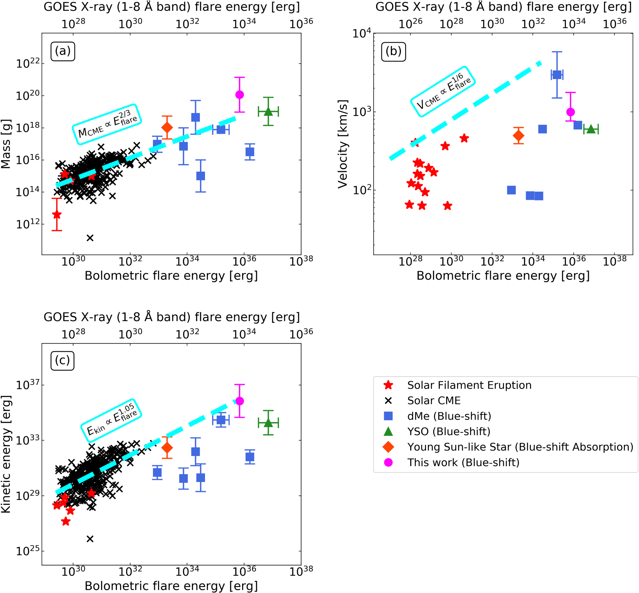
Figure 8(a) indicates that the erupted prominence on V1355 Orionis has roughly the mass that expected from the scaling law of solar CMEs. This suggests that the prominence eruption on V1355 Orionis was caused by the same physical mechanism as the solar prominence eruptions/CMEs (e.g., Kotani et al. 2023). Figure 8(a) also shows that it is the largest prominence eruption observed by blueshift. These facts may provide important clues as to how a large event can be caused by the physical mechanism of solar prominence eruptions. Our observations may provide an opportunity to understand extreme eruptive events on stars.
Figure 8(b) shows that the prominence velocity on V1355 Orionis is indeed fast, but overwhelmingly below the theoretical upper limit of the velocity (Takahashi et al. 2016) estimated from the flare energy. Therefore, the fast prominence eruption is physically possible to occur in association with a 1035 erg class flare.
Figure 8(c) indicates that kinetic energy corresponds roughly to the value predicted from the scaling law of the solar CMEs. In our calculation, the kinetic energy of the prominence is 4.5 × 1033 erg < K < 1.0 × 1037 erg. As discussed in Moschou et al. (2019), the kinetic energy of the prominence on other stars is smaller than that expected from the scaling law of solar CMEs. The possible reason for this discrepancy is that prominence eruptions generally have a lower velocity than CMEs in case of the Sun (Maehara et al. 2021; Namekata et al. 2022a), although it is also proposed that the suppression by the overlying large-scale magnetic field can contribute to small kinetic energies (Alvarado-Gómez et al. 2018). For the blueshift events except on V1355 Orionis, the kinetic energy tends to be smaller than the scaling law. However, we are not sure if the prominence of V1355 Orionis is below the scaling law due to the large indefiniteness of the kinetic energy.
Given these considerations, the prominence eruption on V1355 Orionis and solar prominence eruptions may have a common physical mechanism. However, the large uncertainties in the mass estimate make it difficult to compare them with the solar CME scaling law. For the mass estimation, we made various assumptions, as discussed in Section 4.1.2, that may be incorrect. A more accurate derivation of the prominence mass requires a simulation as performed in Leitzinger et al. (2022), as well as concerning the two components in Section 4.2.
5. Summary and Conclusion
We simultaneously performed spectroscopic observations in this study using the Seimei telescope and photometric observations using TESS on the RS CVn-type star V1355 Orionis. We captured a superflare that releases 7.0 × 1035 erg and has the following characteristics:
- 1.For the first 30 minutes after the flare started, a pronounced blueshift in the Hα emission line was observed confirming that the prominence eruption occurred in association with the flare.
- 2.The velocity of the prominence eruption calculated from the blueshift was up to 990 km s−1 (one-component fitting) and 1690 km s−1 (two-component fitting), which is well above the escape velocity of 347 km s−1.
- 3.There seems to be two blueshifted excess components with multiple possible interpretations.
- 4.The mass of the prominence eruption is also one of the largest ever observed (9.5 × 10¹⁸ g < M < 1.4 × 10²¹ g), corresponding to the value expected from the flare energy–mass scaling law that holds for solar CMEs. However, the mass estimates make many uncertain assumptions and are highly indeterminate.
In a very rare case, a prominence eruption at the velocity that greatly exceeds the escape velocity of the star was captured continuously at a high temporal resolution of 1 minute simultaneously with a white-light flare. The massive and fast prominence eruption detected in this study provides an important indicator of just how large an eruption the physical mechanism of solar prominence eruptions can cause. This will certainly need to be investigated in the future with a larger sample of prominence eruptions in the energy range of >1035 erg.
As also discussed in Leitzinger et al. (2022), simply applying the empirical relation of solar prominence/filament visibility to a star can involve many ambiguities. Further, modeling and simulation of prominence visibility on K-type stars are necessary to accurately interpret our data, especially the two-peaked blueshifted excess component. This would also contribute to a more accurate derivation of the prominence mass.
The spectroscopic data used in this study were obtained through the program 20B-N-CN03 with the 3.8 m Seimei telescope, which is located at Okayama Observatory of Kyoto University. TESS data were obtained from the MAST data archive at the Space Telescope Science Institute (STScI). All of the TESS data used in this paper can be found in MAST:10.17909/ffwb-dg98. Funding for the TESS mission is provided by the NASA Explorer Program. We thank T. Enoto (Kyoto University/RIKEN), H. Uchida, and T. Tsuru (Kyoto University) for their comments and discussions. We acknowledge the International Space Science Institute and the supported International Team 510: Solar Extreme Events: Setting Up a Paradigm (https://www.issibern.ch/teams/solextremevent/). This research is supported by JSPS KAKENHI grant Nos. 20K04032, 20H05643 (H.M.), 21J00106 (Y.N.), 21J00316 (K.N.), and 21H01131 (H.M., D.N., and K.S.). Y.N. was also supported by NASA ADAP award program No. 80NSSC21K0632 (PI: Adam Kowalski).
Facilities: Seimei (Kurita et al. 2020) - , TESS (Ricker et al. 2015) - .
Software: astropy (Astropy Collaboration et al. 2013, 2018), kools_ifu_red (Matsubayashi et al. 2019), IRAF (Tody 1986), PyRAF (Science Software Branch at STScI 2012)