


Abstract
We investigate the distributions of the obliquity angle and impact parameters of nulling pulsars of different duty cycles based on the simulation of more than 600,000 samples. We adopt a purely geometric approach for pulsar visibility, in which visible emission is emitted tangentially to the magnetic field line and parallel to the line-of-sight direction. The geometry is incorporated with the model for pulsar magnetospheres of multiple emission states, in which the plasma charge density is dependent on the emission state. We assume that an emission state can only exist between two limiting conditions described by the vacuum and corotation models, respectively. In this model, pulse nulling corresponds to emission switching to a state in which the plasma charge density is zero. The event is detectable only if the switching occurs at source points that lie on a trajectory, whose locus defines the locations of visible emission, within an open-field region. Our results show that detectable nulling is dependent on all three parameters, such that nulling pulsars prefer a small obliquity angle and duty cycle, and tend to have positive impact parameters. We find that the total population of nulling pulsars in our samples is around 23%, of which about 47% possess a duty cycle of 0.1 or smaller. The former implies that there are more nulling pulsars than currently known. Our model predicts that the number of nulling pulsars increases as the obliquity angle decreases, which also implies that the occurrence of nulling in a pulsar should evolve over time.
Export citation and abstract BibTeX RIS

Original content from this work may be used under the terms of the Creative Commons Attribution 4.0 licence. Any further distribution of this work must maintain attribution to the author(s) and the title of the work, journal citation and DOI.
1. Introduction
A relatively common single-pulse event observed in radio pulsars exhibits an abrupt cessation of the entire pulse emission for a duration of several pulsar rotations to minutes (Backer 1970; Rankin 1986; Wang et al. 2007; Young et al. 2015). Known as pulse nulling, there are more than 100 pulsars that have been reported with such behavior (Sheikh & MacDonald 2021). To quantify the phenomenon, Ritchings (1976) introduced a parameter known as the nulling fraction (NF), which is derived from the fraction of pulses without detectable emission (Gajjar et al. 2012). This allows the investigation of correlations between nulling and other pulsar parameters based on the NF in different pulsars. An example relates to the suggestion that the null pulses appear to increase with the pulsar's age. Assuming that the pulsar age is correlated with the rotation period, Ritchings (1976) concluded that the NF is related to the rotation period of a pulsar, such that pulsars with longer periods possess higher NFs (Biggs 1992; Wang et al. 2007). Even though knowing that the NF for a pulsar is useful, the parameter does not give specific information for the separation of the nulls in time or the duration for each null state. In addition, very little information about the emission geometry can be derived from NFs.
Later investigations suggested that nulling should be a common phenomenon present in half of the known pulsars. From the study of 60 pulsars, whose data were drawn from other observations performed at different frequencies ranging from around 145–1420 MHz, Rankin (1986) found that the NF is related to the morphology of the integrated profiles in different pulsars (Biggs 1992). By separating profiles into different classes, small NFs were found in pulsars with pulse profiles of a single component (Weisberg et al. 1986), whereas high NFs were found in pulsars that possessed profiles with multiple components. For a given profile class, the correlation between the NF and the pulsar age was not identified, and pulsars with greater age did not show larger NFs than those possessing smaller NFs. Furthermore, Rankin (1983) suggested that young pulsars are likely to have small NFs because their profiles are dominated by a core component. This implies that the apparent relationship between nulling and age is the result of differences between core single and conal profile classes in different pulsar ages. Biggs (1992) further suggested a correlation between the NF and the obliquity angle such that the former is large when the latter is small. From a statistical study of nulling pulsars, Li & Wang (1995) concluded that the NF shows more correlation with the pulse width, or duty cycle, than with the rotation period or the obliquity angle. This suggests that nulling may have a geometric origin.
Another piece of information relating to pulse cessation comes from the observations of intermittent pulsars. Emission of the pulsars exhibits two states of emission on, when pulses are detectable, and off, in which pulses are nondetectable (Kramer et al. 2006; Camilo et al. 2012; Lorimer et al. 2012; Lyne et al. 2017). The quasi-periodic emission is interpreted as switching in the magnetospheric plasma density between two emission states of ample and vacuum (Kramer et al. 2006). The suggested correlation between emission and plasma density is consistent with the popular view that radio emission is generated from highly relativistic plasma. The outward streaming of the plasma along the open field lines in two-stream instability implies that the pulse intensity is proportional to the plasma density (Manchester & Taylor 1977; Cordes 1979; Lyubarskii 1996). Although a widely accepted model for changes in the plasma density is still lacking, a model for an obliquely rotating pulsar magnetosphere consisting of multiple quasi-stable emission states of differing charge density has been put forward (Melrose & Yuen 2014). The model is based on an interpolation of the plasma charge density between two limiting conditions. One limit corresponds to the corotation, in which the charge density is the Goldreich & Julian (1969) density, ρGJ, as described by the corotation model. The other limit corresponds to the vacuum-dipole model, in which the inductive electric field,
E
ind, is specified by the rotating magnetic dipole. We interpret the screening of the parallel component of
E
ind as due to a charge density,  , of arbitrarily small value, such that there are too few charges to provide the potential field implied by corotation. We consider a class of emission states described by the parameter y, such that the plasma charge density is a combination of y proportion of
  and (1 − y) times ρGJ. In the model, variation in the plasma charge density is signified by changes in the emission state, which are parametrized by changes in the value of y.
Most of the literature has focused on the correlations between the nulls (or the NFs) and other pulsar properties for characterization of the pulsar emission mechanism and its evolution over time (Ritchings 1976; Lyne & Ashworth 1983; Rankin 1986; Wang et al. 2007; Gajjar et al. 2014b; Sheikh & MacDonald 2021). There have been suggestions that the NF alone may not carry enough information to describe nulling pulsars, and that other parameters may need to be taken into account (Sheikh & MacDonald 2021). In this paper, we investigate the distribution of the obliquity angle, α, between the rotation and the magnetic axes, and the impact parameter, β = ζ − α, where ζ is the viewing angle between the line of sight and the rotation axis (Radhakrishnan & Cooke 1969), for different duty cycles, δ, and their correlations with pulse nulling pulsars based on simulation of a large sample of pulsars. In addition, the relationship between pulse nulling and the pulsar emission geometry is examined. For simplicity, we assume that nulling is a manifestation of pulse cessation due to a change in the plasma density without considering the underlying mechanism and the duration, or frequency, of the nulls. We assume a purely geometric model for pulsar visibility in which observable emission emits tangentially to the dipolar magnetic field lines, whose footpoints are located in the open-field region (Cordes 1978; Hibschman & Arons 2001; Kijak & Gil 2003), and parallel to the line-of-sight direction (Gangadhara 2004; Yuen & Melrose 2014). In this case, analytic expressions are available for the parameters in our simulation. Our investigation involves the simulation of different profile widths, or duty cycles, each being identified as the range of pulsar phase between which visible emission comes from the open-field region. Doing so requires determining the emission height that can satisfy the designated duty cycle for a given pulsar. From the analysis based on polarization position angles derived from a large population of pulsars (Rankin 1993; Tauris & Manchester 1998), the distribution of the obliquity angle was shown to lie within the range of α ≲ 90° with the population highly concentrated toward small values (Rankin 1990). The result has been supported by different simulations (Zhang et al. 2003; Kolonko et al. 2004). In addition, investigations of the intermittent pulsars also gave predictions for their obliquity angles within the same range (Gurevich & Istomin 2007; Lorimer et al. 2012), even when the different particle acceleration models were taken into account (Li et al. 2014). Therefore, we consider α in the range between 0° and 90°. Radio emission has been shown to come from a relatively higher height at around 0.1rL or above (Johnston & Weisberg 2006), where rL = c/ω⋆ is the light-cylinder radius and ω⋆ is the spin frequency of the star. Here, we assume a maximum height of 0.2rL. We focus on the emission that forms the main pulse without referring to the interpulse.
This paper is organized as follows. In Section 2, we outline the model for pulse nulling. The steps for the simulation and the results are given in Section 3, and the correlations between nulling pulsars and the pulsar parameters are investigated in Section 4. We discuss and conclude the paper in Section 5. The relevant electromagnetic fields are outlined in Appendix A, and the transformation matrices are given in Appendix B.
2. Cessation of Visible Emission
In this section, we outline the model for pulse cessation and the geometry for the detection of nulling.
2.1. Model for Pulse Cessation
We assume a pulsar magnetosphere with multiple different emission states. Each of the emission states is specified by a particular value in the parameter y between two limiting conditions signified by 0 and 1, respectively (Melrose & Yuen 2014). In this model, the electric field for an emission state possesses the form given by

where the electric field associated with the corotation charge density is given by  , and
b
is the unit vector along the dipolar field lines.
E
ind signifies the inductive electric field, which is due to an obliquely rotating magnetic dipole. The expression for
E
ind is defined by Equation (A2). The case for y = 0 corresponds to the corotation electric field,
E
=
E
cor, given by Equation (A5) as described by the corotation model (Goldreich & Julian 1969). The case represented by y = 1 is associated with the minimal model, in which
E
ind∥ is screened and
E
ind⊥ has the same value as in the vacuum-dipole model. This requires the presence of a charge density,
, and
b
is the unit vector along the dipolar field lines.
E
ind signifies the inductive electric field, which is due to an obliquely rotating magnetic dipole. The expression for
E
ind is defined by Equation (A2). The case for y = 0 corresponds to the corotation electric field,
E
=
E
cor, given by Equation (A5) as described by the corotation model (Goldreich & Julian 1969). The case represented by y = 1 is associated with the minimal model, in which
E
ind∥ is screened and
E
ind⊥ has the same value as in the vacuum-dipole model. This requires the presence of a charge density,  , to generate an electric field so that
  , with

A charge density is required to screen the electric field along the magnetic field lines for all emission states between the minimal and the corotation states. This implies a screening charge density for an oblique rotator given by Melrose & Yuen (2014)

with

representing the corotation charge density (Goldreich & Julian 1969) for y = 0. The screening happens provided that the creation of the secondary pairs results in a multiplicity, λ, greater than unity (Beskin et al. 1993; Melrose & Yuen 2012). This implies λ = e(n+ + n−)/ρGJ ≫ 1 (Gurevich & Istomin 2007), where ρGJ = e(n+ − n−) and n± are the number density of positrons and electrons. In an obliquely rotating magnetosphere with multiple emission states, the plasma density is given by  . The proposal that pulsar radio emission as produced from highly relativistic plasma flowing out along the open field lines in two-stream instability suggests that the pulse intensity is proportional to the plasma density (Manchester & Taylor 1977; Cordes 1979; Lyubarskii 1996). The correlation between plasma density and pulse intensity implies that the latter is proportional to
  . Assuming identical λ in different emission states suggests that the pulse intensity is proportional to
  in our model. Therefore, a change in the value of y corresponds to a change in
  resulting in variation of the observed pulse intensity. The cessation of the visible pulse emission is then modeled as a sudden change in the emission state, corresponding to a change in the y value to y = yN, in which the plasma charge density is zero (
 ).
).
In order for changes in the pulse intensity to be detectable, changes in  are required to occur at the locations from where emission is visible. The visible pulse emission is assumed to originate from a geometry, in which radiation is emitted from the open-field region and observable emission is directed tangentially to the dipolar magnetic field lines at the source point (Cordes 1978; Hibschman & Arons 2001; Kijak & Gil 2003) and parallel to the line-of-sight direction. The location of the visible point (θbV, ϕbV) in the magnetic frame (subscript b) at a particular pulsar phase, ψ, for a given ζ and α is defined by Gangadhara (2004) and Yuen & Melrose (2014) as
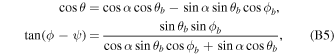
where  . The (θbV, ϕbV) pairs can be expressed in the observer's frame (θV, ϕV) using Equation (B5). The values of θbV and ϕbV change as a function of ψ tracing a path that closes after one pulsar rotation, referred to here as the trajectory of the visible point. The solutions relevant to our simulation are obtained from the nearer of the two magnetic poles relative to ψ = 0, where the impact parameter, β = ζ − α, is minimum. The assumption that emission occurs only within the open-field region introduces the dependence on height. For a given ζ and α, there exists a minimum height, rV, for which the trajectory is tangent to the locus of the last closed field lines given by Yuen & Melrose (2014):

Here, the polar angle of the point on the last closed field line is represented by θbL, and θL designates the angle between the rotation axis and the point where the last closed field line is tangent to the light cylinder. Equation (6) suggests dependence of the visible point on height, with the range of visible emission coming from a point for r = rV and increases with increasing r − rV. The center of the profile window is located at ψ = 0°, where the line of sight, the magnetic axis, and the rotation axis are coplanar.
2.2. Observable Emission
The location for an observable emission in the magnetosphere may be defined uniquely by assuming that the emission is only from the last closed field lines. Then, the radial distance to any points on the field line at ϕb from the stellar center can be determined using Equation (6), with polar angles given by the trajectory of the visible point. Therefore, observable emission is specified by (rV, θV, ϕV) on each of the last closed field lines in the magnetosphere. For an oblique rotator, these parameters vary with ψ (see Appendix B), with rV having its minimum and maximum at ψ = 0 and ψ = 180°, respectively. This implies that emission is from higher (lower) altitudes at the edges (center) of a profile (Gangadhara & Gupta 2001; Karastergiou & Johnston 2007).
The height of the source of radio emission is poorly determined, and is usually estimated based on (i) relativistic phase shift, with the requirement of an asymmetric pulse profile that possesses a clearly defined cone and core components (Dyks et al. 2004), or (ii) geometry, with the emitting source located on the last closed field lines (Kijak & Gil 2003). Here, we assume model (ii), which implies that emission is visible from only one point in the magnetosphere for any given ψ. For highly relativistic emitting particles with a large Lorentz factor γ, the emission is confined to a narrow forward cone with a half angle to the magnetic field line given by 1/γ. This is a small angle due to aberration such that some spread in emission exists about the direction tangent to the field line. In particular, emission is expected to come from a small range of field lines inside the last closed field line, and this translates into emission over a corresponding small range of heights r > rV.
2.3. Detection of Nulling
From the model outlined in Section 2.1, emission is visible provided that the emission source lies on the trajectory of the visible point, and the trajectory lies partly (or entirely) inside the open-field region, and the pulse width is the range of ψ over which this condition is satisfied. The boundary of this region is defined by the locus of the last closed field lines, which satisfy  for 0 ≤ ϕb
< 2π, with r0 = rL. This suggests that the boundary of an open-field region is dependent on both r and ψ, with visible emission coming from height r only when the trajectory of the visible point is inside this boundary. The latter implies a pulse width that is given in terms of the range of ψ on the trajectory inside the open-field region. The profile edges are defined by the points of intersection between the trajectory and the boundary of the open-field region. Assuming the points of intersection defined by ψ1 and ψ2 would mean that the pulse width is given by Δψ = ψ2 − ψ1, or a duty cycle δ = Δψ/2π. Pulse cessation corresponds to the existence of the emission state given by yN such that
for 0 ≤ ϕb
< 2π, with r0 = rL. This suggests that the boundary of an open-field region is dependent on both r and ψ, with visible emission coming from height r only when the trajectory of the visible point is inside this boundary. The latter implies a pulse width that is given in terms of the range of ψ on the trajectory inside the open-field region. The profile edges are defined by the points of intersection between the trajectory and the boundary of the open-field region. Assuming the points of intersection defined by ψ1 and ψ2 would mean that the pulse width is given by Δψ = ψ2 − ψ1, or a duty cycle δ = Δψ/2π. Pulse cessation corresponds to the existence of the emission state given by yN such that  for each ψ in the range of the locations defined by Δψ. A pulsar is considered a nulling pulsar when the emission region suddenly switches in the emission state from y = yE ( ≠ yN) to y = yN, then back to y = yE, where 0 ≤ {yN, yE} ≤ 1.
The relationship between the geometry of visible emission and nulling is illustrated in Figure 1. The nulling region signified by  with 0 ≤ yN ≤ 1 for α = 30° is illustrated in gray in the magnetic frame. Three trajectories of the visible point using the same α but different ζ values are also shown in different colors. The trajectory in brown does not intersect with the nulling region meaning that nulling in this pulsar will not be detectable. Part of the green trajectory around ψ = 0° lies inside the nulling region indicating that pulse cessation is potentially detectable (if the phenomenon occurs). Similar conclusions can also be made for the trajectory in blue. The difference between the trajectories in green and blue is in the range of ψ (profile width) for observable emission that lies inside the nulling region. To demonstrate that, Figure 1 also shows the boundary for an open-field region assumed at 0.2rL. Emission is only observable if the trajectory is within the boundary. As shown in the figure, the blue trajectory cuts the nulling region from A to B at ψ = ∓102°, respectively, but it cuts the open-field region from
  to
to  at ψ = ∓65° giving a duty cycle of about 0.36 for detectable nulling. For the trajectory in green, it begins to cut the open-field region at
  at ψ = −77°, where it is outside of the nulling region. It does not enter the nulling region until ψ = −60° at C, from where it stays inside through to D at ψ = 60°. After that, the trajectory traverses the open-field region (non-nulling region) from D to
  and exits at
  at ψ = 77°. The total duty cycle is 0.43, but with pulse cessation detectable for only about 78% of the whole profile. This means that pulse cessation as seen along the green trajectory does not satisfy our definition of nulling. It also follows that for a given δ, for example, δ = 0.2, detection of nulling across the whole profile is possible only for the blue trajectory.
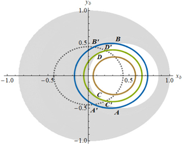
Figure 1. Plot illustrating the nulling region in gray for α = 30° in the magnetic frame where the magnetic pole is located at the origin. Also shown are three trajectories of the visible point using the same α but with ζ = 25° (brown), 35° (green), and 45° (blue). The boundary of an open-field region at 0.2rL is shown as a dotted black curve centered at the origin. While all the trajectories traverse the open-field region, only the blue and green trajectories cut the nulling region. For them, the entry and exit locations at the boundary of the nulling region are indicated by A, B, C, and D, and those for the open-field region are indicated by the same letters with a prime.
Download figure:
Standard image High-resolution image3. Simulation and Results
Our investigation for the correlation of nulling with the duty cycle (δ), the obliquity angle (α), and the impact parameter (β) is based on simulation. The preparation of the different parameters is as follows. For each δ from 0.1–1.0, in steps of 0.05, different combinations of {ζ, α} are obtained from iterating over the range of 1° ≤ α ≤ 90°, in steps of 0 5, and over the range of 0° ≤ ζ ≤ 90°, also in steps of 05. This gives 32,399 different combinations of {ζ, α} (corresponding to the same number of pulsars) for each δ. We assume that all pulsars are capable of emission state switching, and each is emitting in an emission state of a particular y = yE value between 0 and 1. The condition for pulse nulling then involves (i) solving for y = yN such that
  , and (ii) the value of yN must lie between 0 and 1, inclusively. The pulsar is then assumed with the capacity of multiple switching between yE and yN indefinitely without considering the NF. The specific calculations follow the steps below:
- 1.
- 2.For each δ, ψ1 and ψ2 are determined assuming that the fiducial plane is at ψ = 0°.
- 3.Equation (3) is then used to determine the yN value, which satisfies
 for each ψ between ψ1 and ψ2.
 - 4.For a given δ, a nulling is considered valid for a combination of ζ and α only if the y = yN value between 0 and 1 can be identified for each ψ.

We obtained a total of 647,980 sample pulsars in the simulation.
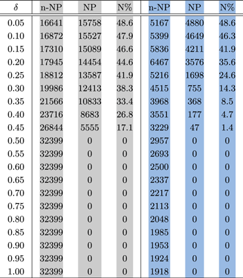
Table 1 shows the statistics for the nulling pulsars compared to non-nulling pulsars for each δ obtained from the simulation. Here, we consider two cases: (i) unrestricted β and (ii) ∣β∣ ≤ 15° and r ≤ 0.2rL. The former sets a limit on the results, and β in the latter case is chosen for consistency with the results for the shape of radio beams obtained from analysis of the mean pulse profiles, and the associated polarizations, in the pulsar data (Lyne & Manchester 1988). To implement a restriction on the emission height, Equation (6) is used to calculate the height along the trajectory of the visible point for a given δ. Only the combinations of ζ and α are considered if the heights are below 0.2rL. For unrestricted β and δ ≤ 0.1, the numbers of non-nulling and nulling pulsars are roughly identical. As δ increases, the percentage of the nulling pulsars begins to drop reaching zero for δ ≥ 0.5 in our simulation. The implication of δ = 1.0 is that emission is observable from a single pole (see Esamdin et al. 2005 for an example). This restricts α to small values. A similar decrease in nulling percentage is observed when restrictions are put on β and the emission height, but the decrease is greater as δ increases, reaching zero for δ ≥ 0.5. Since pulsars can have virtually any α value, Table 1 may be considered as a simulation for all pulsars in the range of 1° ≤ α ≤ 90° for different δ values. For unrestricted β, we obtain 111,899 out of a total of 647,980 samples giving 17.3% of nulling pulsars. When restrictions are imposed, there are 20,361 nulling pulsars out of a total of 88,354 samples, or about 23.0% that exhibit nulling. The higher proportion is the result of the restrictions that put a limit on the pulsars with visible emission and this applies to both nulling and non-nulling pulsars. This can be seen from the decrease in the pulsar number for each δ, with the decrease increasing as δ increases. The current approximation is 8% of the known pulsars with nulling (Sheikh & MacDonald 2021), which is lower than our predictions. From the non-nulling pulsars and nulling pulsars shown in the blue shaded columns in Table 1, if we assume that a typical duty cycle for ordinary pulsars is ≲0.1 (Manchester & Taylor 1977; Maciesiak et al. 2011), then the ratios of nulling pulsars below and above that are roughly equal, at 47% and 53% of all the nulling pulsars.
Table 1. Statistics for Non-nulling and Nulling Pulsars for Different Duty Cycles (δ)
|
Note. The impact parameters are selected such that (i) all samples are included (columns in gray) and (ii) ∣β∣ ≤ 15° (columns in blue). For case (ii), the maximum emission height is also implemented at 0.2rL. Here, n-NP and NP are acronyms for non-nulling and nulling pulsars, respectively, and N% represents the percentage of pulsars with nulling for a particular δ.
Download table as: ASCIITypeset image
4. Correlations with the Pulsar Parameters
In this section, we examine the correlations between pulse nulling and β, α, and δ. We ignore the cases for δ ≥ 0.5, as the number of nulling pulsars is zero, and consider only the distributions with ∣β∣ ≤ 15° and r ≤ 0.2rL imposed.
4.1. Distributions of α and β
Figure 2 shows the variation in the distribution of α for nulling and non-nulling pulsars for four different δ values. For δ = 0.1, the distribution for nulling pulsars is almost unchanged for α ≲ 75°, beyond which the number begins to drop and reaches zero at α = 90°. As δ increases to 0.2, the total number of nulling pulsars decreases, and the distribution reaches a minimum value at α ∼ 40° and increases again as α increases, resulting in two peaks at α = 1° and α ∼ 75°. From δ = 0.3–0.4, the overall distribution shrinks and shifts toward smaller values of α. In addition, virtually no nulling pulsar is found for α ≳ 40° at δ = 0.3, which decreases to α ≳ 10° for δ = 0.4. The reasons for this change in the distribution are twofold. First, the decrease in the distribution as α increases is increasingly unlikely for pulsars with a broad pulse width while emission remains coming from lower heights. This also applies to non-nulling pulsars, as shown by the progressive decrease in the distribution in gray. Second, this is also because nulling, with the requirement that the yN value lies between 0 and 1, over a larger δ is becoming increasingly rare. This is illustrated in Table 1 from the decrease in the number for both nulling and non-nulling pulsars as δ increases. It follows that pulsars demonstrating nulling over a large δ are likely to have small α. In addition, there exists a range of α below about 5°, where the number of nulling pulsars remains the highest in all the distributions. It is clear from Figure 2 that the number of nulling pulsars is dependent on both δ and α. An alternative presentation of that is given in Figure 3, which shows the variation in the normalized number of nulling pulsars as a function of δ ≤ 0.5 for nine α intervals. The rate of decrease in the number is unique for different α intervals. For example, the decrease in numbers as δ increases is different for pulsars with α around 5° (light blue) and 45° (cyan), with the decrease being larger in the latter.

Figure 2. Histograms showing the distribution of α for four different δ at 0.1, 0.2, 0.3, and 0.4 from top to bottom, respectively, under the conditions of ∣β∣ ≤ 15° and r ≤ 0.2rL. The nulling and non-nulling pulsars are indicated by blue and gray, respectively. The total number of both the nulling and non-nulling pulsars tends to decrease as δ increases, and their corresponding distributions increasingly shift toward small α.
Download figure:
Standard image High-resolution image
Figure 3. Plot showing the variation in the normalized number of nulling pulsars for nine α intervals. In the legend, the interval ranges are shown, in which a square bracket signifies that the value at the starting point is included, and a parenthesis is used to indicate that the ending point is not included. The variation in the number of nulling pulsars is such that it decreases as δ increases with a rate that is different for different α intervals.
Download figure:
Standard image High-resolution imageThe variation in the distribution of β is shown for four different δ in Figure 4. For δ = 0.1, the distributions of nulling and non-nulling pulsars are divided at β ≈ 1° with the former distribution concentrated in the positive region. As δ increases, the number of nulling pulsars decreases but their β remains mostly positive. This can be seen in Figure 1, where the trajectory with β < 0 (brown) tends to lie outside of the nulling region compared to trajectories with β > 0. In Figure 4, the percentages of nulling pulsars with negative β are 0.11%, 0.14%, 0.66% and 2.82% for δ = 0.1, 0.2, 0.3, and 0.4, respectively. On the contrary, the β for the non-nulling pulsars spans increasingly evenly across the positive and negative β as δ increases. For the chosen ranges of ζ and α, our results show that non-nulling pulsars can possess β of different signs, whereas β is positive for the majority of the nulling pulsars.

Figure 4. Similar to Figure 2, but for the distribution of β. While the distribution of non-nulling pulsars (in gray) increasingly spreads equally in the positive and negative β values as δ increases, the distribution of nulling pulsars (in blue) remains mostly in the positive β.
Download figure:
Standard image High-resolution image4.2. Nulling and the Emission Geometry
From Figure 2 for nulling pulsars, the changes in a roughly even distribution across a large range of α at δ = 0.1 to increasingly concentrating toward small α as δ increases imply that nulling pulsars tend to have low α values. This is shown in Figure 5, which is obtained from adding together all nulling pulsars in Table 1. There is a clear peak in the distribution at around α = 1°. The distribution then decreases as α increases and becomes roughly constant for 30° ≲ α ≲ 75°, beyond which it drops again reaching zero at α = 90°. We find that 50% of the nulling pulsars possess α with a value less than 355 in our simulation, and 80% with α ≤ 635. The weighted average of α is 376. For comparison, we cross-referenced the list given by Lyne & Manchester (1988) for pulsars with known estimated α values with the nulling pulsars in the literature. We identified 55 such nulling pulsars (see Table 2 in Appendix C), of which about 51% of them possess α ≤ 355 and around 78% have α ≤ 635, which are in close agreement with our results. It is believed that evolution of α is correlated with the pulsar age based on the consideration of energy loss through the magnetic-dipole radiation of an oblique rotator (Manchester & Taylor 1977; Lyubarskii & Kirk 2001). This implies that pulsar braking decreases as α approaches zero, where there is no electromagnetic radiation, and the evolution of α is toward a smaller value as a pulsar ages. The more nulling pulsars with small α lead to the conclusion that nulling is correlated with the pulsar age. In our model, such correlation is related to the emission geometry outlined in Section 2. As α increases, the range of θ covered by the nulling region decreases, and the overall location in θ increases. The former means that the size of the nulling region shrinks, and the latter implies that its height in the magnetosphere increases for large α. It follows that the θV values of the trajectory of the visible point must also be large enough, which means large heights from Equation (6), in order to cut the nulling region. Since radio emission is believed to come from the inner magnetosphere, the result is that the number of nulling pulsars with large α is less than that with small α. If ignoring the underlying mechanism, the above suggests that the nulling region evolves as the pulsar ages, and a pulsar without nulling (due to large α) may exhibit nulling at a later stage in its evolution.

Figure 5. Total distribution of α for all the nulling pulsars in the blue column in Table 1.
Download figure:
Standard image High-resolution image
5. Discussion and Conclusions
We have investigated the relationship between pulse nulling and three pulsar parameters (obliquity angle, impact parameter, and duty cycle) based on the simulation of more than 600,000 samples. Pulse nulling is defined as the plasma charge density dropping to zero in an emission state that lies between the two limiting conditions described by the minimal model, in which the parallel component of the inductive electric field is screened by  , and the corotation model, in which the plasma charge density has the value in Goldreich & Julian (1969). The detection of nulling is based on a purely geometric model defined by ζ and α, which dictates the trajectory of a visible point in the magnetosphere. The trajectory then cuts the open-field region within which emission is visible. Nulling is detectable provided that the change in the plasma charge density, corresponding to a change in the emission state, occurs along the trajectory of the visible point for a given profile width. For different duty cycles, we determined the statistics for the number of nulling pulsars for restricted and unrestricted impact parameters, with the former also having a maximum emission height at 0.2rL imposed. We found that nulling pulsars tend to have a duty cycle of 0.1 or below, and they are likely to possess small obliquity angles.
Pulse nulling is interpreted in our model as changes in the plasma charge density due to switching in the emission state. The proposed changes involve y = yE to y = yN, then back to yE, and the corresponding changes in  is from
  (emitting) to
  (nulling) to
  (emitting). One may refer to the emission condition where
  as true pulse nulling because there is truly no charge density for generating the radiation. From Figure 1, this condition is satisfied only for certain regions in the magnetosphere, and
  anywhere else. A situation arises in which the value of
  may be very low, but not zero, and so is still capable of generating weak emission. By definition, this is not nulling in our model. However, the intensity of the emission may be lower than the flux density threshold of some telescopes, and consequently reported as nulling. This may correspond to the trajectory in brown in Figure 1, where it does not cut the region of
  but it may traverse a region in which such weak emission is generated. Another feature of this model is that the change in emission can be related quantitatively to the changes in y. The above also implies that the emission state before and after a null is the same, which is given by yE. However, this may not always be the case. Consider nulling in PSR B0809+74, with which observation showed that the drift rate of subpulses changes when the pulsar nulls with an accompanying change in phase of the post-null average profile (van Leeuwen et al. 2003). This suggests that the y value before and after a null is different. This example illustrates how observations of nulling may be used to estimate the change in the value of y. As shown in Section 2, such treatment would also require the knowledge of ζ and α, and realistic estimates of the two parameters are possible only with high-quality data.
Simultaneous single-pulse studies showed that pulse nulling in some pulsars is a broadband phenomenon, and that concurrent nulling behaviors were detected at different observing frequencies (Taylor et al. 1975; Bartel & Sieber 1978; Bhat et al. 2007; Gajjar et al. 2014a), although contrary views have also been reported (Bartel et al. 1981; Davies et al. 1984). The suggestion that emissions at different frequencies may be associated with emitting sources locating at distinct heights in a magnetosphere possessing field lines of a dipolar-like structure gives rise to the well-known radius-to-frequency mapping (Cordes 1978). The mapping states that radiation at higher frequency comes from lower height, and vice versa. Our model for pulsar visibility, as outlined in Section 2.1, implies that visible emission at a given frequency comes from only one height with the location given by (rV, θV, ϕV). From Figure 1, a higher height (larger rV value) would correspond to a trajectory with the locus occupying larger values in the (xb , yb ) coordinates. For the case considered in the figure, the trajectory may still cut the nulling region but at different locations. Our definition of nulling, as due to switching in the value of y such that yE → yN → yE, may or may not occur simultaneously across the entire nulling region. If it does, then correlated pulse nulling will be detected across different frequencies. However, it is also possible for some pulsars that state switching at different parts of the magnetosphere is not concurrent, and this will result in the observed nulling (if it occurred) not being correlated across different frequencies.
The proportion of nulling pulsars as evaluated in our samples is 23% when restrictions are put on β and emission height, with ∣β∣ ≤ 15°, to be consistent with observations (Lyne & Manchester 1988), and height ≤ 0.2rL (Johnston & Weisberg 2006). This is higher than reported by the latest investigations (Sheikh & MacDonald 2021). The difference is partly due to our assumption that all pulsars can exhibit state switching. The increasing number of pulsars with observed switching in the emission properties (Smits et al. 2005; Kramer et al. 2006; Rankin et al. 2006; Lyne et al. 2010; Camilo et al. 2012; Lorimer et al. 2012; Keith et al. 2013; Marshall et al. 2015; Lyne et al. 2017; McSweeney et al. 2017) suggests that sudden changes of some kind in pulsar magnetospheres may be common. Important information from these observations is that the timescale of switching is different for different pulsars, and for different phenomena. It illustrates that some pulsars may have switching timescales that are too long to be detected in regular observing sessions. It suggests that pulsars with emission switching should be more common, which agrees with our assumption. It then follows from our results that the observed fraction of nulling pulsars should be larger. It is possible that some pulsars may have NFs that are too small, or too large, to be detected by observations of average duration. Then, the discovery of such nulling pulsars is dependent on the observing time. However, as mentioned above, it may also be that nulling in some pulsars requires high-quality data to discern the subtle drop in the pulse intensity from the originally very weak emission. Our use of the traditional criterion for nulling being equivalent to emission cessation across the whole pulse profile (Backer 1970; Wang et al. 2007) clearly rules out other nulling behaviors. It is likely that some pulsars, with certain combinations of ζ and α, may exhibit nulling that does not conform with the traditional definition. An example relates to the observation of PSR J1819+1305 (Rankin & Wright 2008), which showed nulling only in the last component of the three-component profile. It also indicates that nulling can take place across only a range of longitudinal phases within the profile. This means that nulling is a complex phenomenon, and the exact number of nulling pulsars may be greater. Subsequently, a more complete survey of their population is in favor of long observing sessions using powerful telescopes, such as the 500 m Aperture Spherical radio Telescope (FAST) and the future Square Kilometer Array (SKA). The raw sensitivity of FAST, given by the ratio of the effective collecting area to the system temperature, is nearly three times that of the Arecibo telescope (Nan & Li 2013), meaning that the flux density threshold is much lower than that of most radio telescopes. For example, FAST has already discovered a few pulsars with interesting emission patterns. This includes PSR J2338+4818, which is potentially an intermittent pulsar (Cruces et al. 2021), and PSR J0344-0901, which shows mode-changing behavior (Cameron et al. 2020). There is no doubt that more nulling pulsars with increasing complexity will be discovered, which will enrich our understanding of the pulsar radio emission mechanism.
We thank the XAO pulsar group for useful discussions, and R. Bamnbasom for the critical reading of the manuscript. We also thank the anonymous referee for valuable suggestions that improved the presentation of this manuscript. R.Y. is supported by the Key Laboratory of Xinjiang Uygur Autonomous Region No. 2020D04049, the National SKA Program of China No. 2020SKA0120200, the Natural Science Foundation of China (grant Nos. 12041304, U1838109, 11873080, 12041301), the 2018 Project of Xinjiang Uygur Autonomous Region of China for Flexibly Fetching in Upscale Talents, and partly supported by Xiaofeng Yang's Xinjiang Tianchi Bairen project and CAS Pioneer Hundred Talents Program.
Appendix A: Electric and Magnetic Fields
An obliquely rotating time-dependent magnetic dipole, μ , produces a vector potential, A , of the form given by Melrose & Yuen (2014):

where x is the position vector from the stellar center, and r = ∣ x ∣. The corresponding inductive electric field is given by

In spherical coordinates, Equation (A2) has the form given by
We note that
E
ind is proportional to  and so it is absent for an aligned rotator. The magnetic field equation is given by
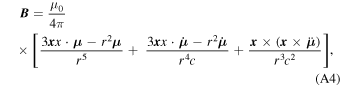
where the terms ∝ 1/r2 and ∝ 1/r are radiative terms, and the term ∝ 1/r3 is dipolar (subscript "dip"). Since μ is a function of α in the observer's frame, all B , E pot, and E ind are also functions of α.
In the comoving frame of a plasma-filled magnetosphere with negligible particle inertia and infinite conductivity, the electric field vanishes giving

Equation (A5) represents the corotation electric field (Goldreich & Julian 1969), and ω ⋆ is the rotation frequency of the star. For an obliquely rotating magnetosphere, Equation (A5) may be written as (Hones & Bergeson 1965; Melrose 1967)

where E ind = − ∂ A /∂t. In spherical coordinates, E cor has only components along the radial and polar directions and perpendicular to the dipolar field lines.
Appendix B: Coordinate Transformations
We adopt the arrangement of the rotation and magnetic axes of a pulsar in Cartesian coordinates in such a way that  and
and  , respectively, and the corresponding unit vectors are given by
  and
and  . Transformation between the unit vectors is given by
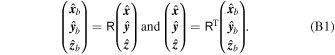
Here,
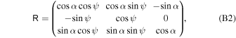
and R
T is the transpose of R. The equivalent unit vectors for radial, polar, and azimuthal in spherical coordinates are described by  and
and  , and the transformation is given by

with
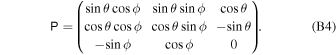
Transformation of the angles between the magnetic and the observer's frames is given by
and
Appendix C: Some Nulling Pulsars
This section lists some of the known nulling pulsars in the literature (for example, see papers by Wang et al. 2007 and Konar & Deka 2019) with the estimated obliquity angle given by Lyne & Manchester (1988).
Table 2. The 55 Nulling Pulsars with Estimated α
| PSR | α° | PSR | α° | PSR | α° | PSR | α° | PSR | α° |
|---|---|---|---|---|---|---|---|---|---|
| B0148-06 | 15.5 | B0149-16 | 90.0 | B0301+19 | 31.9 | B0329+54 | 30.8 | B0450-18 | 31.1 |
| B0523+11 | 49.1 | B0525+21 | 23.2 | B0538-75 | 23.0 | B0628-28 | 15.8 | B0656+14 | 8.2 |
| B0736-40 | 17.7 | B0818-13 | 90.0 | B0823+26 | 13.1/26.1 | B0826-34 | 2.1 | B0834+06 | 60.7 |
| B0835-41 | 54.0 | B0940-55 | 19.6 | B1055-52 | 17.9 | B1133+16 | 51.3 | B1154-62 | 17.5 |
| B1237+25 | 48.2 | B1451-68 | 23.5 | B1508+55 | 80.0 | B1642-03 | 68.2 | B1700-32 | 47.0 |
| B1706-16 | 55.3 | B1718-32 | 87.2 | B1727-47 | 86.9 | B1737+13 | 40.8 | B1738-08 | 28.7 |
| B1747-46 | 90.0 | B1749-28 | 57.8 | B1819-22 | 17.0 | B1821+05 | 27.7 | B1839+09 | 90.0 |
| B1845-19 | 59.8 | B1857-26 | 20.9 | B1907+03 | 6.5 | B1911-04 | 71.2 | B1917+00 | 78.2 |
| B1918+19 | 14.0 | B1919+21 | 45.4 | B1929+10 | 6.0 | B1933+16 | 64.9 | B1942-00 | 29.2 |
| B1946+35 | 43.1 | B2003-08 | 12.7 | B2016+28 | 40.4 | B2020+28 | 71.2 | B2044+15 | 40.7 |
| B2045−16 | 36.7 | B2111+46 | 8.6 | B2154+40 | 22.4 | B2310+42 | 33.5 | B2319+60 | 19.0 |
Download table as: ASCIITypeset image