


Abstract
The Solar Probe ANalyzer for Ions (SPAN-I) onboard NASA's Parker Solar Probe spacecraft is an electrostatic analyzer with time-of-flight capabilities that measures the ion composition and three-dimensional distribution function of the thermal corona and solar-wind plasma. SPAN-I measures the energy per charge of ions in the solar wind from 2 eV to 30 keV with a field of view of 247 5 × 120° while simultaneously separating H+ from He++ to develop 3D velocity distribution functions of individual ion species. These observations, combined with reduced distribution functions measured by the Sun-pointed Solar Probe Cup, will help us further our understanding of the solar-wind acceleration and formation, the heating of the corona, and the acceleration of particles in the inner heliosphere. This paper describes the instrument hardware, including several innovative improvements over previous time-of-flight sensors, the data products generated by the experiment, and the ground calibrations of the sensor.
Export citation and abstract BibTeX RIS

Original content from this work may be used under the terms of the Creative Commons Attribution 4.0 licence. Any further distribution of this work must maintain attribution to the author(s) and the title of the work, journal citation and DOI.
1. Introduction
Parker Solar Probe (PSP) is a robotic NASA mission designed to make the closest ever in-situ measurements of the Sun. The three-axes stabilized spacecraft will orbit the Sun with an initial aphelion slightly inside Earth's orbit. Through several Venus gravity assists, PSP will decrease its perihelion from 35 solar radii (Rs ) to 9.68 Rs using a total of 24 orbits within a seven-year time frame. Data collection is configured such that the primary, high-cadence measurements occur during closest approach (10–15 day span), while the remaining time is spent in cruise phase with a low measurement cadence. The mission objectives are summarized by the following three core components: (1) Determine the structure and dynamics of the magnetic fields at the sources of the fast and slow solar wind, (2) trace the flow of energy that heats the solar corona and accelerates the solar wind, and (3) explore mechanisms that accelerate and transport solar energetic particles. Further information on the scientific goals and measurements can be found in Fox et al. (2016). The SPAN-I instrument is part of a larger ensemble of plasma sensors called the Solar Wind Electrons, Alphas, and Protons (SWEAP) investigation. SWEAP consists of two electron electrostatic analyzers (ESA and SPAN-E; Whittlesey et al. 2020), one ion ESA (SPAN-I), and a Faraday cup (SPC; Kasper et al. 2016; Case et al. 2020).
SWEAP is designed to characterize the phase-space distribution functions of the solar-wind and coronal plasmas with the greatest possible completeness and detail within modern technological abilities. Completeness is driven by the desire to observe and distinguish the large-scale structures and solar-wind conditions in all regimes of the PSP encounters. Given a continuous record of the plasma conditions on each orbit from SWEAP, it is possible to study the evolution and interaction of corotating solar-wind streams, the propagation of transients, and more broadly the connection from the corona through the inner heliosphere. This course of study is key to the closure of mission objectives (1) and (3), and the SWEAP contribution complements those of all four instrument suites. Detail is driven by the desire to measure the plasma microstate and spatiotemporal fluctuations that signify the wave–particle and kinetic processes governing energy transport. These are the keys to the solar-wind heating and acceleration problem described in mission objective (2) of Fox et al. (2016).
The SPAN and SPC instruments are designed to be complementary to one another with respect to phase-space coverage. The SPC instrument, which faces the Sun and measures charged particle fluxes within a ∼30° field of view (FOV), is optimized for the measurement of positive ions in the outer phases of the encounter where solar-wind flows are primarily radial in the spacecraft frame. The SPAN instruments are designed to measure ions and electrons beyond that FOV. SPAN-Ion is optimized for ion observations near the closest approach, where the inflow may be strongly nonradial in the comoving frame due to the extremely high orbital speed of the spacecraft, which will be as high as 190 km s−1.
The SPAN-A sensor is mounted toward the bottom of the spacecraft bus and behind the thermal protection system (TPS). SPAN-A is mounted with a 20° rotation around the spacecraft z-axis. The FOV plot on the right shows the spacecraft in red and the SPAN-I small and large anodes along ϕ and the deflection angles along θ. As expected, there is a partial replaced coverage blockage of anode 0 due to the TPS and the fully extended (90°) solar panels. The result is that only a partial measurement is made of the true ion flux, the correction of which is an ongoing project using in-flight calibration data. This obstruction is not present for all anode 0 measurements as there are deflection angles that point away from the spacecraft–Sun line.
2. The Ion Solar Probe Analyzer
The SPAN-Ion instrument uses an ESA and a time-of-flight (TOF) mass discriminator to resolve ambient ions by their incident angle, energy per charge, and mass per charge (see Figure 1). Figure 2 shows the mounting configuration of the instrument relative to the spacecraft bus and the resulting field-of-view. field of view. SPAN-I is able to separately resolve the 3D distribution functions of H+ and He++, and has some additional capability of measuring higher-mass-per-charge elements. The dynamic range of the instrument is increased by a mechanical attenuator at the analyzer aperture and an electrostatic spoiler that reduces the signal within the ESA.

Figure 1. Left: SPAN-A flight module with the right (SPAN-I) and left (SPAN-E) ESA. SPAN-I consists of an ESA with deflectors followed by a titanium TOF section for mass-per-charge discrimination. Right: SPAN-I separated from the main SPAN-A unit.
Download figure:
Standard image High-resolution image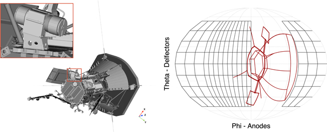
Figure 2. Left: Parker Solar Probe spacecraft with the SPAN-A sensor highlighted in the red box. Right: Mollweide projection of the SPAN-I field of view, including partial obstruction of the spacecraft and its TPS (red). The projection is based on the look direction of the anodes in ϕ and the deflector angles in θ.
Download figure:
Standard image High-resolution imageAs shown in the block diagram of Figure 3, ions are first selected by elevation angle by the deflecting electrodes and are then filtered by energy per charge as they pass through the top-hat electrostatic analyzer. Once they exit the ESA, ions are further accelerated by an additional energy of −15 kV into the TOF analyzer to resolve their respective mass per charge by using a START/STOP double coincidence measurement. Ions entering the TOF will have an original energy per charge with an additional of 15 keV before they encounter a set of carbon foils that generate a pair of START and STOP secondary electrons. The START electrons are accelerated by the optical design toward the inner portion of the TOF and ultimately impinge on the microchannel plate (MCP) detectors; similarly for the STOP electrons which originate from the STOP foil directly above the MCPs. The short delay (7–200 ns) between the START and STOP signals and the short transit gap (2 cm) allows for a measurement of the post-accelerated particle velocity. The resulting electron cloud from the MCP collects on the anode below it and passes through a constant fraction discriminator (CFD) to make an accurate time measurement, independent of the pulse amplitude. Then, the signal is transmitted to the digital board below the anode board that contains an application-specific integrated circuit (ASIC) to convert signals from high-speed time difference to digital values. A full block diagram of the electronic components is shown in Figure 3 followed by a description of the individual electronics boards (see Figure 4). A summary of the instrument performance parameters and design characteristics are shown in Table 1.
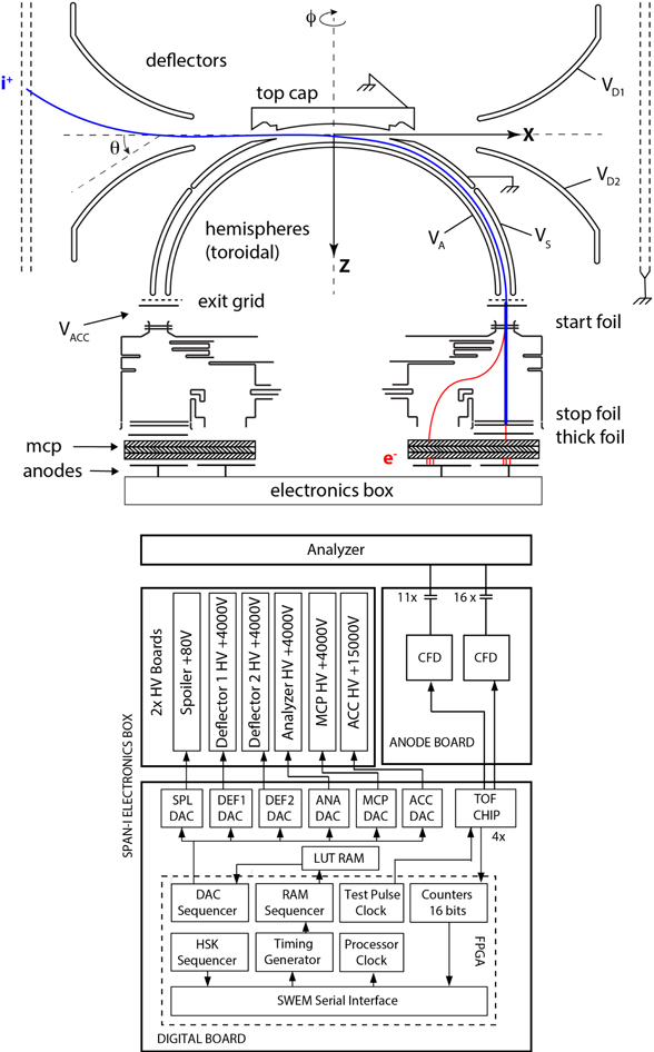
Figure 3. Block diagram of the SPAN-I sensor, including ESA, TOF, and individual components of the electronics box.
Download figure:
Standard image High-resolution image
Figure 4. Left figure: Back side of each individual board that is part of the electronics box. The top row shows the anode board, the digital board, and the high-voltage board. The bottom row shows the second high-voltage board, the low-voltage power supply, and the backplane. Right figure: Front side of each individual board in the same configuration as in the figure to the left.
Download figure:
Standard image High-resolution imageTable 1. SPAN-I Instrument Design Parameters
| Parameter | Value | Comments |
|---|---|---|
| ΔR/R | 0.033 | Toroidal top hat a |
| Analyzer radii | R1 = 3.34 cm | Inner hemisphere toroidal radius |
| R2 = R1 ∗ 1.030 = 3.440 cm | Outer hemisphere toroidal radius | |
| R3 = R1 ∗ 1.639 = 5.474 cm | Inner hemisphere spherical radius | |
| R4 = R3 ∗ 1.060 = 5.803 cm | Outer hemisphere spherical radius | |
| RD = 3.863 cm | Deflector spherical radius | |
| Opening angle hemisphere | 13° | |
| Opening angle top cap | 12° | |
| Analyzer constant | 16.7 | As derived from the optics model |
| Analyzer voltage (max) | 0–4000 V | Controllable to less than 1 V |
| Deflector voltage | 0–4000 V | Controllable to less than 1 V |
| Spoiler voltage | 0–80 V | Set to zero by default (no attenuation) |
| Energy range | 2 eV–30 keV | |
| Analyzer energy resolution | 7% | |
| Spoiler attenuation factor | 10 b | Setting for E1 & E2; varies with the energy channel |
| Post analyzer acceleration | −15 kV | |
| Carbon foil thickness | <1.5 μg cm−2 | Differs for each anode |
| Carbon foil grid frames | 333 lines inch−1 | 62% transmission |
| TOF gap between START/STOP | 2 cm | |
| Thick foil | 500 nm Kapton | 50 nm Al coating |
| Carbon Foil START efficiency | 50% | |
| Carbon Foil STOP efficiency | 23% | |
| Energy sweep rate | 32 steps in 0.218 s | |
| Deflector sweep rate | 8 steps / 32 "microsteps" in 6.80 ms | "Microsteps" in full sweeps only |
| Spoiler sweep rate | 32 steps in 0.218 s | Only when enabled—zero by default |
| Azimuth range | 2475 | |
| Instantaneous field of view | 2475 × 3507 | θ = 0° (no deflection) |
| Field of view each sweep | 2475 × 120° | |
| Anode angle resolution | 1125 or 225 | 10 Small STOPs—6 large STOPs—11 Large STARTs |
| Analyzer geometric factor | 0.00105cm2 sr eV | Simulations for 2475 analyzer only |
| 5.984 × 10⁻⁴ cm2 sr eV | Including 5 × 90% transparency grids | |
| Measurement cadence | 0.435 s | For either Full or Targeted Sweeps (not both) |
| Measurement duration | 0.218 s | For 32 energy by 8 deflector bins |
| Counter readout | 0.852 ms | 32 energy by 8 deflector bins per sweep |
Notes.
a Note that the values in the above table are as designed values; final calibrated values to be included in a future SPAN-I calibration special issue paper. b Estimated, final calibration pending spoiler used in Encounter 3 and beyond.Download table as: ASCIITypeset image
SPAN-I draws significant heritage from the STATIC sensor on Mars Atmosphere and Volatile EvolutioN (MAVEN), which was designed to measure Martian atmospheric ions and the solar wind. The primary difference between these instruments lies in the geometric factor, which in the case of SPAN-I was reduced in order to avoid saturation of the detector near the Sun. This was accomplished by decreasing the hemispherical gap size and thus reducing the ΔR/R. The concern for saturation was addressed with the addition of an electrostatic "spoiler" (see section below) to further reduce the geometric factor by a factor of 10. While SPAN-I is built to measure H+ and He++ of the solar-wind composition, the sensor also detects higher-mass ion species such as O6+ and Fe7+. Both SPAN-I and STATIC differ from previous TOF mass spectrometers by their smaller design (<3.3 kg), large dynamic range in both energy and particle flux, and in its simplified electronics that do not require floating detectors at the TOF acceleration potential of −15 kV. Details of the instrument subsystems are described below.
2.1. Electrostatic Analyzer
SPAN-I's electrostatic analyzer (ESA) geometry draws its heritage from the STATIC instrument on the MAVEN spacecraft (McFadden et al. 2015). The top-hat toroidal approach to ESAs (Carlson et al. 2001) used for SPAN-I was originally designed for the Cluster mission (Reme et al. 1997) and successfully flown on the FAST satellite (Klumpar et al. 2001). The advantages of the top-hat design are its large geometric factor, optimal field of view, adequate energy resolution (dE/E 7%), and optics that allow exiting ions to be properly imaged by subsequent sectors. For SPAN-I, the electrostatic focal point is shifted from the exit grid of the ESA to the entrance of the −15 kV acceleration region to optimize the particle throughput within the TOF optics. The ESA's outer hemisphere is held at ground while the inner section is biased up to −4 kV, which provides an energy range between 125 eV and 20 keV for the first encounters. UV sunlight contamination and particle scattering off of the outer surface is reduced with the addition of Ebanol-C coating and scalloping features. As the exit of the ESA is close to the −15 kV HV acceleration sector, it is necessary to add a pair of grids at the exit of the ESA in order to reduce fringe fields. In front of the ESA aperture are two deflectors that allow the elevation angle of the instrument to be increased by up to +/−60° at energies as high as 4 keV per charge.
2.2. Electrostatic Deflectors
In front of the ESA aperture are two deflectors that allow the elevation angle of the instrument to be increased by up to +/−60° at energies as high as 4 keV.
2.3. Attenuators
SPAN-I is capable of measuring a large dynamic range of particle fluxes in the solar wind by using two modes of attenuation: a mechanical attenuator and an electrostatic spoiler. The mechanical attenuator is mounted between the deflectors and the ESA aperture. Before and during launch, the attenuator remains in a closed position, together with the one-shot TiNi cover, to prevent detector contamination and acoustic damage to the carbon foils. After launch, the cover is opened and the mechanical attenuator is allowed to move the multislit metal shield in and out of the ESA FOV by using a series of nanomuscle shape-memory alloy (SMA) actuators. The slits allow a reduction in ion fluxes by a factor of 10. In addition to the mechanical attenuator, SPAN-I includes an electrostatic spoiler, serving as an additional electrode that forms the lower half of the outer hemisphere (the upper half is maintained at ground). When the spoiler is held at a particular voltage (maximum of 80 V), the distribution of ions traveling through the analyzer is reduced by electro-optically narrowing the energy per charge passband. Initial calibration testing has shown the spoiler to be capable of reducing the ion flux to background levels, assuring an additional safety mechanism for saturation of the detector. Final calibration of the energy-dependent geometric factor is yet to be determined. Both attenuator mechanisms are under software control that monitors specific instrument parameters, such as counting rates and system attenuator state. Once the count rate exceeds a preset threshold, a set of logical and sequential combinations of the attenuation mechanisms are activated to maintain an ideal count rate. When transitioning the mechanical attenuator, the actuating nanomuscles require a 5 minute relaxation time to allow for thermal settling.
2.4. Time of Flight
The mechanical TOF design is a direct copy of the TOF used on STATIC/MAVEN. The design uses two sets of carbon foils for both the START and the STOP signal generation, which simplifies the mechanical design by allowing a separation of the TOF HV region (−15 kV) from the MCP detector voltage (3 kV). In order for ions with a mass per charge heavier than H+ and He++ to penetrate two carbon foils with high enough efficiencies, we selected ultrathin foils (<1 μg cm−2) combined with a post-acceleration voltage of −15 kV. The −15 kV TOF HV supply also produces a secondary voltage (11/12 of the full voltage), enabling the deflection of secondary electrons generated by the first set of carbon foils toward the START anodes below the TOF section. The carbon foils at the entrance and exit of the TOF analyzer are additionally shielded by grids to suppress field emissions generated by impurities and tears within the carbon foils.
ACF-Metals was the primary provider of the carbon foils. The production begins with the foils mounted on standard mica slides, which were placed on top of a cantilever base and lowered into a hot-water bath containing a surfactant solution. The floating carbon foil is then retrieved by replacing the now empty glass with the stainless steel frame containing a 333 line/inch grid mesh and raising the cantilever base above the water surface. Once removed, the foils were vacuum baked and then scanned for impurities using software developed for the MAVEN mission. The selection process of the foils included a thorough review of the high-resolution scans, the associated software results, and a calibration test using ion species of different mass per charge values.
2.5. Anode Board
The SPAN-I anode board is located below a Z-Stack MCP configuration and detects the START and STOP electrons. The flight MCPs have a resistance of 45 MΩ and a nominal gain of 2–3 × 10⁷. The gain is adjustable by controlling the MCP bias voltage through software commands and is continuously monitored in flight by performing multiple MCP-Gain tests at every encounter. The electron cloud generated at the bottom of the MCP is collected by a series of 11 inner discrete anodes (STARTs) and 16 outer discrete anodes (STOPs). Each of the 27 discrete anodes is connected to a dedicated CFD located close to the anode to reduce the signal travel time. The CFD enables high-resolution timing-of-arrival signals independent of the input pulse amplitude. The 11 inner (START) anodes have an angular size of 225 spanning a total azimuthal FOV of 2475. The 16 outer anodes (STOPS) are separated into 10 high-resolution anodes (1125) and 6 larger anodes (225). The STOP anodes permit a finer azimuthal resolution and are aligned such that the higher-resolution area is pointed toward the solar-wind direction.
2.6. Digital Board
The SPAN-I digital board contains the main instrument field-programmable gate array (FPGA) and four individual TOF chips, each having four input signals from both a START and STOP CFD for a combined 16 TOF measurements. The TOF chip acquires the input signals from the CFDs and passes on the processed results to the FPGA for further analysis. The FPGA is the main processing unit of the instrument and includes functions such as command execution and science data production. It communicates directly with the SWeap Electronics Module (SWEM), using the provided storage for data archiving and potential delivery to the spacecraft. The digital board also houses a set of MRAM and SRAM memory, where the digital-to-analog converter (DAC) control values for the HV components, the associated sweeping tables, and data acquisition schemes are stored. More about the instrument data acquisition scheme is detailed in Section 3.
2.7. High-voltage Power Supply Board
There are two SPAN-I high-voltage power supply boards (HVPS) that operate the HV electrodes of the instrument. The first HVPS supplies high voltage to the hemisphere, spoiler, and both deflectors with voltage values controlled and set by a digital-to-analog converter (DAC) chip with a 4 V reference on the digital board. The stepping, or sweeping, from one voltage value to another, occurs every 0.2 ms for the full sweep (0.8 ms for the targeted sweep) with a voltage settling time of <1 ns. The second HVPS supplies high voltage to the MCPs and the TOF section, once again set via DACs, but held at nominal values pending further calibration. For the deflector supplies, however, the DAC is referenced relative to the hemisphere supply control voltage. Using this coupled DAC control voltage technique results in deflector biases scaled to the correct value for each hemisphere voltage step.
2.8. Low-voltage Power Supply Board
The LVPS generates 1.5V, 3.3V, +/−5V, +/−8V secondary voltages from the 22V supplied by the SWEM. As a fail-safe mechanism, the 22V source is routed through the backplane to a socket with a high-voltage enable plug. RIO ASIC monitors are also mounted to monitor the voltage and current draws.
2.9. Backplane Board
The SPAN-I backplane board has several functions: 1. Provide high-voltage signals to the spoiler and deflector; 2. Transmit actuation commands to the cover mechanism and mechanical attenuator; 3. Provide access to the enable plug for ground testing and instrument safety.
3. Measurement Operations
3.1. Voltage Sweeps
SPAN-I is designed to perform a sweeping sampling of ions at a constant rate. A sweep is composed of either 1024 steps (Full) or 256 steps (Targeted), changing the instrument optics with each step by altering associated voltages and therefore sampling specific regions of phase space. There are a total of four sweeps that occur every "New York" second, which is derived from a 19.2 MHz clock and subdivided into bins to form an integration time of 224/19.2 × 106 (0.874 s). A sweep therefore happens every 218.45 ms, alternating between a Full sweep and a Targeted sweep. A Full sweep uses high-voltage steps that allow for a coarse mapping of the entire range of the energy per charge space with the drawback of having regions where the spectrum is not sampled. This drawback is addressed with the Targeted sweep. Once the Full sweep is completed, the FPGA determines which bin contained the maximum number of counts and selects the appropriate Targeted table for a high-resolution scan around this region. Full sweeps contain a total of 1024 steps, which are reduced to a 256 bin product by summing to every fourth step (microstepping). The Targeted sweeps do not have microstepping and simply step through 256 bins in the same amount of time. Figure 5 shows example sweeps of the Full and Targeted data acquisition modes.

Figure 5. Sample sweep diagram for a Full (top) and a subsequent Targeted (bottom) sweep. The black circles represent 4096 possible combinations of the hemisphere and both deflectors settings. The blue line shows the path that the sweep takes, beginning with deflector voltages (and microstepping) and then stepping by hemisphere voltage. Once the Full/coarse sweep is complete, a Targeted sweep around the peak value (in this case red crosses) is performed.
Download figure:
Standard image High-resolution image3.2. Sweep High-voltage Lookup Tables
Each of the four high-voltage electrodes (hemisphere, deflectors, spoiler) sweeps through voltages to sample the ambient plasma. The sweeping mechanism is controlled by the FPGA, which reads DAC values from lookup tables residing on the instrument SRAM memory and sets the voltage accordingly. There are a total of one HV lookup table (LUT) and two index LUTs: the Sweep HVLUT, Full IndexLUT, and Targeted IndexLUT. The Sweep LUT contains the 4 DAC values for controlling the hemisphere, the spoiler, deflector 1, and deflector 2. These values are all interspersed so that a reference to the start address of the first DAC setting locates the remaining three DACs. There are a total of 4096 DAC values, 16 bits long, for each of the four electrodes. The Sweep LUT is referenced with two tables, the Full–LUT and the Targeted LUT, which contain the correct indexes to perform a "coarse" and "targeted" measurement, respectively. The Full–LUT contains 1024 index values for the 1024 steps it sweeps through during a single cycle, with a microstepping feature that reduces the product to 256 bins by summing every fourth step. The Targeted LUT, on the other hand, contains 256 index values for the 256 steps it sweeps through during a targeted sweep cycle. Targeted sweeps focus around the previous high-voltage step where the peak counts occurred. Therefore, there are 256 separate tables of 256 indexes in the Targeted LUT based on the 256 steps where the peak can occur.
3.3. TOF Operations
The TOF measures the time between START and STOP pulses from a single anode for a particular angle and energy per charge. The value measured is originally a value between 0 and 2047 representing the delays of 0 to 208.33 ns. Each count of the output represents 101.725 ps in delay, such that a value of 512 from the TOF converts to a value of 52.1 ns in delay. Before the TOF value is passed onto the data processing unit the FPGA either accepts the 9 most significant bits (MSBs) of the TOF, discarding the 2 least significant bits (LSBs), or it compresses the 10 MSB into 9 bits (discarding the LSB). The compression scheme is N for counts less than 256, N/2+128 for counts between 256 and 511, and N/4+256 for counts greater than 511. This compression emphasizes TOF resolution at low TOF values. The TOF value is further categorized into a mass per charge value by using a mass lookup table (MLUT) derived from ground calibration. For each energy per charge setting the 9 bits of the compressed TOF (cTOF) values are indexed into a 512 element table. Instead of using the full range of high-voltage settings for each energy per charge step (65536), the MLUT uses 128 tables based on the 7 most significant bits of the hemisphere DAC. The table converts the TOF values into 64 distinct mass per charge bins.
3.4. Archive and Survey Products
The first step in generating science products is converting the time-of-flight measurement to a mass per charge. Ions entering SPAN-I are first filtered by their energy per charge, meaning that the particle travel time will change for each energy step across the 2 cm TOF gap. For each energy per charge setting, a separate lookup table is used to convert the particles time of flight into one of 64 distinct mass per charge values. The next table, the Mass–Range–LUT, categorizes the 64 mass per charge bins into four separate mass products defined as: 0-Protons, 1-Alphas, 2-Higher M/Q, 3-Background. Finally, after the particle mass is categorized into a mass range, the FPGA will use a Mass–Bins–LUT to determine how much mass resolution to keep for each ion product. The result is an address space in memory defining a specific ion mass that will be filled with the appropriate science values.
The second step converts the high-voltage steps (energy and elevation), the anode number (azimuth), and the product number (mass address) into an address to increment and be filled with count measurements. The resulting products are then summed over a programmed number of sweeps (either all Full sweeps or all Targeted sweeps) defined in a Sum–LUT table that holds the exponent (n) of a 2n value.
3.5. Single Measurement
The SPAN-I analyzer performs a single high-voltage sweep in 0.248 s, during which a set of voltages are applied to the hemisphere, deflectors, and spoiler based on a sweep lookup table. The first step within the sweep sets the hemisphere voltage to its highest value and subsequently steps through the remaining 31 values logarithmically toward the lowest voltage. For each hemisphere step, the deflectors are stepped through a series of voltages in order to scan in elevation for a specific energy per charge. Lastly, a spoiler voltage is set for each hemisphere step in order to reduce the total flux of incoming particles.
4. Ground Calibration
4.1. Analyzer Response and TOF Efficiencies
A slow rotation scan is performed across all 16 anodes with a 1 keV residual gas beam and −15 kV TOF acceleration. This is to test the azimuthal analyzer response and the associated START and STOP carbon foil efficiencies, which are a measure of the carbon foil secondary electron production efficiency as a function of the ion mass. Multiplying the START and STOP efficiency yields a measure of the total efficiency of the TOF section. The analyzer response function for each individual anode is shown in Figure 6 on the left. The anodes are drawn proportional to one another, but not to scale, and the normalized calibration measurements overlay the corresponding azimuthal angles. For larger anodes 225 (10–15) the relative efficiency is close to 90% with 5% cross talk interference between adjacent anodes. For the smaller STOP anodes of 1125 (0–9) a start anode of 225 is shared, and the signal is divided into its separate components. In this case, the cross talk between anodes is larger and closer to 30% while the relative efficiency stays high. The right side of Figure 6 shows the same anode configuration with carbon foil efficiencies for the STOP and START signals overlaid. The carbon foil efficiencies are derived from the following equation:


where STARTeff (STOPeff) is the START (STOP) efficiency, ValidRate is the valid events rate, and the StartRate (StopRate) is the valid START (STOP) rate. The results show a fairly consistent carbon foil efficiency for both START (50%) and STOP (23%) across all anodes. At the edge of each anode pair there is a slight drop in both efficiencies due in part to the aforementioned cross talk and grids within the TOF section that are in the sensor's FOV. Cosmic rays and radioactive decay background is found to be minimal due to coincidence measurements with ion fluxes as high as 20 kHz.
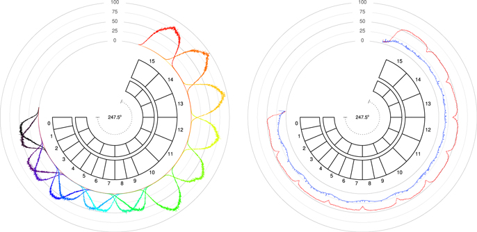
Figure 6. Left: Normalized instrument response function for each anode, where both the START and STOP anodes are displayed. STOP anodes 0–9 are paired with a single START anode in order to increase the angular resolution. For higher-resolution anodes, the effects of cross talk are enhanced relative to the larger anodes. Right: START (red) and STOP (blue) TOF efficiencies for all anodes.
Download figure:
Standard image High-resolution imageIn order to avoid ion feedback and to improve the signal, a 500 nm thick Kapton foil was included after the second set of thin carbon foils. Ions that have passed through both thin carbon foils with an energy of >15 keV are stopped by the thick foil, whereas secondary electrons pass through almost unhindered. The improved signal comes from the scattering of the secondary electrons themselves as the pass through the thick foil, where the narrow beam is now spread over a greater area on the MCP and therefore reduce MCP droop.
The secondary electron yields of protons and helium are estimated to be two electrons from the thin carbon foils (Goruganthu & Wilson 1984; Ritzau & Baragiola 1998). Higher masses, with the same acceleration potential, will typically yield higher numbers of secondary electrons. A more detailed discussion can be found in McFadden et al. (2015). More calibration of efficiencies for different mass species and acceleration will follow in order to improve Venus flybys.
4.2. Analyzer Concentricity
The analyzer concentricity is verified using a series of energy scans for each anode separately. Figure 7 shows test results for anodes 0–3, with the analyzer sweeping logarithmically from 5 eV–20 keV in order to verify the peak tracking mechanism for large energy steps in the full sweep. The top panel represents the targeted scan with peak tracking enabled, while the bottom panel represents the full sweep. Both panels show a clear tracking of the energy beam, even during instances when the beam energy was in between two full sweep energy bins.
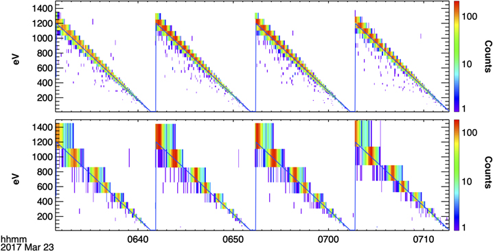
Figure 7. Energy scan of anodes 0, 1, 2, and 3. Ion gun energies are swept from 1200 eV down to zero while the instrument sweeps in energy logarithmically from 5 eV to 20 keV. The ion gun energy is overplotted in blue. Top: Targeted product. Bottom: Full product.
Download figure:
Standard image High-resolution imageThe analyzer k-factor is derived for each anode separately and is shown in Figure 8. Conversion of energy bins from instrument values to physical units in eV is achieved by assuming a linear relationship between the hemisphere voltage and the energy of the particle (k-factor)

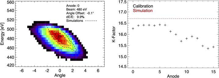
Figure 8. Left: Energy–angle diagram showing the response function of the sensor to a 480 eV ion beam. The instrument simulations are overplotted in black dashed lines. Right: SPAN-I voltage sweep k-factor for all 16 anodes. The red dashed line represents the simulated value of 16.7.
Download figure:
Standard image High-resolution imageThe results show a consistent k-factor for the first six anodes that closely matches the expected simulated value of 16.7. Anodes 7–15 appear to be slightly lower in value, highlighting a slight nonuniformity between the two concentric plates.
4.3. TOF Calibration
The TOF system is verified by testing the mass per charge resolution of individual ion species for a series of different energies. Figure 9 shows the ion travel time in nanoseconds for 1 keV H+,  , He+, N+, O+, Ne+,
  , and Ar+. A clear separation is visible between H+ and
  by up to 4 orders of magnitude, where
  is a proxy of He++ in the solar wind. The
  are measured to be 15% and 20% H+ and
  , respectively. This value slightly changes for different particle energies and is taken into account using the mass–energy lookup table. SPAN-I is also capable of measuring higher-mass species such as O+ and CO2
+, which is ideal for measuring escape ions during the Venus gravity assists.
, respectively. This value slightly changes for different particle energies and is taken into account using the mass–energy lookup table. SPAN-I is also capable of measuring higher-mass species such as O+ and CO2
+, which is ideal for measuring escape ions during the Venus gravity assists.

Figure 9. Mass per charge resolution of individual ion species obtained during ground calibration. A clear separation between H+ and  is visible by up to 4 orders of magnitude, which is optimal for separating the 3D velocity distribution function of the solar wind into protons (m/q = 1) and He++ (m/q = 2). The TOF system is also capable of measuring higher-mass species such as CO and CO2.
Download figure:
Standard image High-resolution imageIn order to determine the correct ion travel time, and therefore the true mass per charge of the particle, it is important to include the energy loss component as the ions traverse the carbon foil. The resulting effect is a slower travel time and a broadening of the mass per charge distribution of individual species, commonly known as straggling. The peak of each distribution from Figure 9 is plotted in Figure 10 together with the corresponding ion mass per charge, taken from the calibration measurements of the ion gun. In addition, four simulations are plotted: The black curve represents the ion travel time with no carbon foil present, while the light blue, blue, and purple lines represent simulations using the "Stopping and Range of Ions in Matter" SRIM/TRIM software (Ziegler et al. 2010) using carbon foil thicknesses of 1.5, 1.0, and 0.5 μg cm−2, respectively. The results show an agreement between the SPAN-I TOF results and the results for the 1.0 μg cm−2 foil thickness, indicating a carbon foil thickness twice as thick as the nominal value.
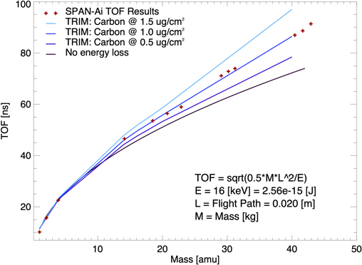
Figure 10. Ground calibration of the travel time for different ion species over the 2 cm TOF gap with an energy of 1 keV (red plus symbols). In addition, three SRIM/TRIM simulations are presented: travel time for 1 keV particles passing through a carbon foil thickness of 0.5 μg cm−2 (purple), 1.0 μg cm−2 (blue), and 1.5 μg cm−2 (light blue). The travel time with no carbon foils is presented in black. The results from calibration match a thickness of 1.0 μg cm−2.
Download figure:
Standard image High-resolution image4.4. On-orbit Operation
Operation of SPAN-I can be divided into two main modes based on spacecraft operations: the primary "encounter" phase of the orbits, which is approximately 10 days centered around PSP perihelion (variable by orbit profile), and the rest of the orbit, hereafter called the "cruise" phase. The instrument measurement rate is higher and uninterrupted during nominal encounter phases as compared to cruise phases, during which the data rate is considerably lower and the measurement periods are interrupted by spacecraft communications, power limitations, and other spacecraft critical operations. During periods of interest (e.g., Venus encounters), the sensors can be configured to collect more data than typically when outside of the encounter.
5. Data Description
SPAN-I data products are classified according to the level of calibration required to produce the files, and the data type that is contained in those files, which are classified by the type of processing required to produce them. Data files are produced in CDF format, available at http://sweap.cfa.harvard.edu/Data.html, and archived in the SPDF.
5.1. Level 0 Data
Level 0 (L0) files are unprocessed files downlinked directly from PSP through the Deep Space Network (DSN) in their original packetized format created by the spacecraft. Files contain a fixed volume of data and are named based on their date of acquisition. On their own, Level 0 files are not useful for scientific analysis but are archived for troubleshooting purposes.
5.2. Level 1 Data
Level 1 (L1) files are converted from the binary L0 format into a format readable by a standard data processing environment, such as IDL or Python packages. SPAN-I uses IDL routines in the data production pipeline to convert L0 files into L1 CDF files. To produce L1 files, minimal processing is performed as the intention of the L1 data is to serve as an archive of the instrument performance in its most raw state. All quantities in the CDF files are in engineering units, e.g., particle counts per accumulation period per energy bin number, deflection bin number, and anode number. Because of the units, L1 files are not useful for scientific analysis. The intention behind archiving L1 files is to keep a record independent from scientific conversions for pipeline debugging purposes and instrument calibration consistency checks over the course of the mission. Housekeeping values are converted into temperatures, currents, and voltages. L1 files are available by request.
5.3. Level 2 Data
Level 2 (L2) data files are generated from L1 files. Instrument units are converted into physical units. For example, the counts per accumulation period are converted into differential energy flux as a function of the energy in electron volts (eV), and deflection and anode bin numbers into degrees in ϕ or θ. The L2 data coordinates remain in the instrument frame of reference. Level 2 data are released to the public for scientific analysis.
5.4. Level 3 Data
Level 3 (L3) products are based on functions performed on L2 files or other processing that expands or reduces the number of dimensions of the L2 data set. Ion moments and fits, which produce values of the density, temperature, and velocity, are classified as L3 products as they are a combination of modified L2 data.
6. Encounters 1 and 2
Parker Solar Probe successfully finished the first two periapsis passes on 2018 November 30 and 2019 April 4, including a Venus gravity assist. The first encounter used an energy sweep table that ranged from 1 keV to 4 keV. We intended to use a sweep table ranging from 125 eV to 20 keV to better capture the solar wind, but due to the discovery of a corrupted sweep table, a backup mode had to be initiated (see Section 7.2 for more details). Prior to encounter 2, new energy sweep tables were uplinked to the spacecraft that set the instrument energy sweep range from 125 eV to 20 keV. A summary of the instrument configurations and product generation are shown in Tables 2 and 3.
Table 2. SPAN-I Instrument Sweep Modes for Encounters 1 and 2
| Mode Name | When Used | Energy Range | # Energy Steps | # Deflector Steps | # Anodes |
|---|---|---|---|---|---|
| Nominal | Encounter 1 | 500eV–2 keV | 32 | 8 a | 8 |
| Nominal | Encounters 2 and 3 | 125eV–20 keV | 32 | 8 a | 8 |
Note.
a Sweep tables used in Encounters 1 and 2 included pre-launch deflector values, and as a result the outermost deflection angles in SPAN-I data are unreliable.Download table as: ASCIITypeset image
Table 3. SPAN-I Data Acquisition Modes from Encounters 1 and 2: Level 1 and 2 Data
| Data | When | Product | Product | Cadence | Anode | Deflection | Energy |
|---|---|---|---|---|---|---|---|
| Type a | Used | Type | Name | (sec) | Bins | Bins | Bins |
| SF00 | Encounter 1 | Proton 3D Spectra | 8D × 32E × 8A | 27.96 | 8 | 8 | 32 |
| SF01 | Encounter 1 | Alpha 3D Spectra | 8D × 32E × 8A | 55.92 | 8 | 8 | 32 |
| SF20 | (Diagnostic) | Proton 3D Spectra | 32E × 64M | 6.99 | ⋯ | ⋯ | 32 |
| SF21 | (Diagnostic) | Alpha 3D Spectra | 32E × 64M | 13.98 | ⋯ | ⋯ | 32 |
| AF00 | Encounter 1 | Proton 3D Spectra | 8D × 32E × 8A | 1.75 | 8 | 8 | 32 |
| AF01 | Encounter 1 | Alpha 3D Spectra | 8D × 32E × 8A | 1.75 | 8 | 8 | 32 |
| AF20 | (Diagnostic) | Proton 3D Spectra | 32E × 64M | 1.75 | ⋯ | ⋯ | 32 |
| AF21 | (Diagnostic) | Alpha 3D Spectra | 32E × 64M | 1.75 | ⋯ | ⋯ | 32 |
| SF00 | Encounter 2 | Proton 3D Spectra | 8D × 32E × 8A | 6.99 | 8 | 8 | 32 |
| SF01 | Encounter 2 | Alpha 3D Spectra | 8D × 32E × 8A | 13.98 | 8 | 8 | 32 |
| SF20 | (Diagnostic) | Proton 3D Spectra | 32E × 64M | 13.98 | ⋯ | ⋯ | 32 |
| SF21 | (Diagnostic) | Alpha 3D Spectra | 32E × 64M | 13.98 | ⋯ | ⋯ | 32 |
| AF00 | Encounter 2 | Proton 3D Spectra | 8D × 32E × 8A | 0.87 | 8 | 8 | 32 |
| AF01 | Encounter 2 | Alpha 3D Spectra | 8D × 32E × 8A | 0.87 | 8 | 8 | 32 |
| AF20 | (Diagnostic) | Proton 3D Spectra | 32E × 64M | 1.75 | ⋯ | ⋯ | 32 |
| AF21 | (Diagnostic) | Alpha 3D Spectra | 32E × 64M | 1.75 | ⋯ | ⋯ | 32 |
Notes.
a Targeted sweep products are not included in this table but have identical formats to their full counterparts; "SF0" is a "Full" energy range product, and "ST0" is its "Targeted" range counterpart. b "S" stands for "Survey", "A" stands for "Archive", "F" stands for "Full", "T" stands for "Targeted".Download table as: ASCIITypeset image
6.1. Encounter 2: Protons
Figure 11 shows proton measurements for all of Encounter 2. The top panel shows the differential energy flux spectrogram of H+ ions summed over all FOV angles. The second panel shows proton measurements along the elevation angle of the instrument (deflectors) summed over the energy per charge and azimuth. The proton flux is clearly centered around 0° corresponding to a plane that aligns with the Sun line. The third panel shows the azimuthal FOV of the instrument, where each bin represents a small (1125) or large anode (225). Anode 0 is currently not included due to its partial obstruction by the TPS. The angle range from 16875 to 180°) requires additional flight calibration in order to determine the correct flux. The last panel shows distance from the Sun in million kilometers.
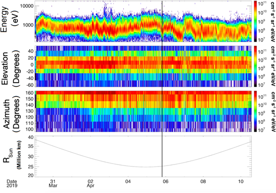
Figure 11. Proton measurements for all of Encounter 2. The top panel shows the energy per charge summed over all look directions, the second panel shows the flux in elevation (deflector sweep), the third panel shows the azimuthal flux (anodes), and the last panel shows the distance from the Sun in million kilometers. The vertical black line marks the time of the data presented in Figure 12.
Download figure:
Standard image High-resolution imageThe 3D VDFs produced by SPAN-I are akin to the ones reported in Marsch et al. (1982), who showcased field-aligned proton beams measured by Helios. Figure 2 of Verniero et al. (2020) similarly demonstrated the evolution of a proton beam during an ion-scale wave storm from Encounter 2. A single time slice, 2019-04-05/19:54:20, from that event is shown in Figure 12. The left panel shows individual energy sweeps for each anode and deflection combination plotted separately with the Alfvén velocity overplotted with a black dashed line. The middle and right panels of Figure 12 represent 2D contour elevations sliced through the ϕ and θ plane, respectively. The black arrow shows the orientation of the magnetic field, where the length of the arrow is the Alfvén speed and the head is placed at the SPC measured solar-wind velocity. Here, we refer to the Alfvén speed of the total proton distribution. Two separate proton distributions are clearly visible: the core and the beam. The "core" is defined as the population centered around the peak in the phase-space density, while the "beam" component comprises the tail.

Figure 12. VDFs from 2019-04-05/19:54:31 showing the core at 350 km s−1 and the beam 600 km s−1, without any interference from He++. Left: phase-space density of H+ for all look directions. Middle: contour elevations showing a 2D slice through the ϕ plane. Right: contour elevations showing a 2D slice through the θ plane. The black arrow represents the magnetic field direction in SPAN-I coordinates, where the head is at the solar-wind velocity (measured by SPC), and the length is the Alfvén speed.
Download figure:
Standard image High-resolution imageThe middle panel of Figure 12 illustrates how much of the proton distribution lies in SPAN-I's FOV; in this particular time slice, we see that the core is partially visible. The 2D cut through the θ plane, in the right panel of Figure 12, reveals a dramatic field-aligned beam featuring a separate peak (green) that is markedly distinct from the core. The left panel of Figure 12 shows that the beam well surpasses the Alfvén speed. Previous observations of VDFs featuring differential flows between different ion populations (Feldman et al. 1973, 1974; Marsch et al. 1982; Marsch & Livi 1987; Neugebauer et al. 1996; Steinberg et al. 1996; Kasper et al. 2006; Podesta & Gary 2011) are known to drive the VDFs unstable, subsequently leading to wave generation (Daughton & Gary 1998; Hu & Habbal 1999; Gary et al. 2000; Marsch 2006; Maneva et al. 2013; Verscharen & Chandran 2013; Verscharen et al. 2013). The preliminary instability analysis conducted by Verniero et al. (2020) underscores the ability for SPAN-I data products to study fundamental processes that govern energy transfer mechanisms in the solar wind, such as wave–particle interactions.
Based on ground calibration, the beam measurement is completely unaffected by the presence of alpha particles at that same energy and are thus resolved without interference. Throughout the encounter, the appearance and disappearance of the proton beam can be attributed to the limited FOV of the instrument, hence the additional presence of SPC.
6.2. Encounter 2: Alphas
He++ measurements can be see in Figure 13. For comparison, the first panel shows the proton spectrogram for Encounter 2. The second panel shows the He++ differential energy flux spectrogram, once again summed over all FOV angles. A clear proton contamination is visible within the data that appear below the He++ distribution. In addition, the highest energy bin contains counts from the energy sweep retrace as the instrument does not engage a dead time during the cycling of the voltage table. Roughly 1% of protons leak into the He++ mass channel and present a large enough contamination that matches the density of He++. This issue is addressed by taking the proton channel and subtracting a time-varying percentage of the flux from the He++ channel. The bottom panel of Figure 13 shows the results of the subtraction algorithm performed on Encounter 2. The proton contamination is greatly reduced, and the He++ distribution becomes apparent.

Figure 13. Energy spectrogram of protons (top), alphas (middle), and alphas corrected for proton bleeding (bottom). Separation between protons and alphas allows for the first individual measurements of the 3D distribution functions of H+ and He++ in the inner heliosphere.
Download figure:
Standard image High-resolution image
7. Instrument Caveats
7.1. Partial 3D Distribution Function
SPAN-I is located behind PSP's TPS and can only observe the partial distribution function of the solar wind. The first 8° closest to the spacecraft z-axis are completely obstructed, meaning that anode 0, which has a 1125 azimuthal size, is 70% covered. For Encounters 1 and 2 the the instrument mostly measured the wings of the solar-wind distribution function, with occasional intervals when the full distribution was visible.
7.2. Table Corruption
During first turn on, it was discovered that one of the instrument sweep tables was corrupted. This was evidenced by the fast housekeeping, which monitors the HV supply, and the resulting failed checksum. This issue was immediately addressed by selecting a backup table to avoid a total loss of data for the first encounter. The backup table has an energy range from 1 to 4 keV, resulting in the solar-wind beam flowing in and out of the instrument energy range.
7.3. Limited Commissioning Time
Commissioning of SPAN-I, including its configuration and HV ramping, was limited in time due to spacecraft maneuvers that placed the Sun behind the heat shield closely after launch and therefore out of the FOV. The spacecraft did perform a transient slew in order to obtain the solar wind into the FOV of SPAN-I, which lasted 20 minutes. The test was used to confirm full functionality of the instrument.
7.4. Protons Bleeding into the Alpha Channel
When ions travel through the TOF they initially collide with the first set of carbon foils that generate the START signal. The interaction with the carbon foil causes a slight loss in kinetic energy; therefore, ions are measured to travel slower than their expected velocity. This straggling effect is especially noticeable in high flux beams such as protons, to the point that enough energy is lost to appear within the alpha product. This issue is addressed for the alpha channel by subtracting a percentage of the proton channel, as straggling protons appear at the same energy per charge in both channels.
7.5. Constant Background and Ghost Peaks
Part of the background that is being measured by the sensor originates within the MCPs, such as radioactive decay of the glass and cosmic-ray penetration. This background was at most 10 Hz and does not significantly contribute to the overall valid events. Another source of constant background comes from coincidence measurements, where the START and STOP pulses are triggered by two different ions. This has been found to be on the order of 1% for fluxes 100 kHz and scales up for larger fluxes (McFadden et al. 2015). Ghost peaks are peaked signals in TOF spectrometers that are found in addition to the expected m/q values but in higher or lower mass bins. Their source is generally attributed to the charge state of ions that exit the carbon foil and to the production of secondary electrons. The SPAN-Ion sensor includes a thick foil placed after the ultrathin STOP carbon foil that prevents several of these spurious ghost peaks to form. For instance, an ion that emerges from the STOP foil as a neutral without generating a secondary electron (30% chance) can generate a valid TOF signal by striking the MCP directly and causing a delayed TOF. This effect is eliminated as the ion will impact the thick foil and generate a nonvalid event that gets filtered by the electronics. Similarly, an ion emerging with a negative charge is also prevented from striking the MCP by the thick foil. While neutral and negative ions are filtered out, positively charged ions still have a small probability of being reflected by the thick foil back onto the carbon foil, thus generating a secondary electron and therefore a delayed TOF. In addition, a molecular ion such as  can breakup at the START carbon foil resulting in particle components that emerge with a smaller kinetic energy and once again a delayed TOF signal. Both of these ghost peaks are seen in the H+ and
  mass peaks in Figure 9.
7.6. High-voltage Sweep Hysteresis
The high-voltage sweeps are arranged so that the hemisphere (energy per charge) is held at a constant voltage value (starting with the highest within the series) while the deflectors are swept in one direction (see Figure 5). When plotting individual energy spectra, a clear hysteresis is observed, where the sweeping of the deflector voltages lags and differs depending on the direction in which it sweeps. This results in a slight offset in the deflection angle from the predetermined table values for alternating energy sweeps. This effect will be addressed in future in-flight calibrations.
8. Conclusion
The SPAN-I sensor will make measurements of the solar-wind 3D velocity distribution function for protons, alphas, and higher-mass-per-charge species within the inner heliosphere. Together with SPC, it will be the first ion sensor since Helios to measure this region and further our knowledge by making the first measurements ever inside of 0.29 au. SPAN-I is a high heritage electrostatic analyzer combined with a mass-per-charge discriminator in order to resolve the underlying physics behind several solar-wind phenomena. This includes tracing the flow of energy that accelerates the solar wind and exploring the mechanics that transport energetic particles. The instrument is situated on the ram side of the spacecraft and can measure the bulk of the solar wind during times of high aberration as the VDF peak enters the instrument aperture. The energy and deflector sweeps are arranged to capture the bulk of the solar wind and are adjustable over the lifetime of the mission in order to adapt to unexplored regimes. The SPAN-I instrument together with the entire SWEAP instrument suite will provide the most complete coverage of the solar-wind plasma in the inner heliosphere and will contribute to observations needed by the scientific community to address outstanding questions of our heliosphere.
This work was funded through work on the NASA contract NNN06AA01C. The authors wish to acknowledge the significant work of all of the engineering staff that worked on the spacecraft and SPAN-Ion instrument, especially Chris Scholz, Matt Reinhart, Andrew Peddie, Other APL folks, and Other UCB folks for their invaluable suggestions on the manuscript.