


Abstract
Our previous linear analysis presents a new instability driven by dust coagulation in protoplanetary disks. The coagulation instability has the potential to concentrate dust grains into rings and assist dust coagulation and planetesimal formation. In this series of papers, we perform numerical simulations and investigate the nonlinear outcome of coagulation instability. In this paper (Paper I), we first conduct local simulations to demonstrate the existence of coagulation instability. Linear growth observed in the simulations is in good agreement with the previous linear analysis. We next conduct radially global simulations to demonstrate that coagulation instability develops during the inside-out disk evolution owing to dust growth. To isolate the various effects on dust concentration and growth, we neglect the effects of back-reaction to a gas disk and dust fragmentation in Paper I. This simplified simulation shows that neither back-reaction nor fragmentation is a prerequisite for local dust concentration via the instability. In most runs with weak turbulence, dust concentration via coagulation instability overcomes dust depletion due to radial drift, leading to the formation of multiple dust rings. The nonlinear development of coagulation instability also accelerates dust growth, and the dimensionless stopping time τs reaches unity even at outer radii (>10 au). Therefore, coagulation instability is one promising process to retain dust grains and to accelerate dust growth beyond the drift barrier.
Export citation and abstract BibTeX RIS

Original content from this work may be used under the terms of the Creative Commons Attribution 4.0 licence. Any further distribution of this work must maintain attribution to the author(s) and the title of the work, journal citation and DOI.
1. Introduction
Growth from (sub-)micron-sized dust grains to kilometer-sized planetesimals is one long-standing problem in planet formation theory. Recently, exploration by the New Horizons spacecraft provided data that constrain planetesimal forming processes at outer radii in the early solar nebula (Stern et al. 2019; McKinnon et al. 2020). The bi-lobe shape of one Kuiper Belt object, Arrokoth, indicates that the object might form via gravitational collapse of a dust clump in the presence of a gas disk. This scenario seems consistent with one proposed scenario of planetesimal formation (see also Nesvorný et al. 2019): streaming instability and subsequent gravitational instability (GI; e.g., Youdin & Goodman 2005; Johansen & Youdin 2007; Johansen et al. 2007; Youdin & Johansen 2007; Bai & Stone 2010; Simon et al. 2016; Abod et al. 2019; Carrera et al. 2021). However, recent studies show that the streaming instability is substantially stabilized by diffusion in gas turbulence (Chen & Lin 2020; Umurhan et al. 2020). McNally et al. (2021) investigated growth rates of the streaming instability in the presence of the turbulent diffusion with dust size distribution. They showed that even weak turbulence with α ∼ 10−5 can quench the streaming instability (see Figure 8 therein), where α is the turbulence strength (Shakura & Sunyaev 1973). Therefore, it is important to investigate other processes potentially leading to outer planetesimal formation, including secular GI (e.g., Ward 2000; Youdin 2005a, 2005b; Shariff & Cuzzi 2011; Youdin 2011; Michikoshi & Kokubo 2012; Takahashi & Inutsuka 2014; Tominaga et al. 2018, 2019, 2020; Pierens 2021).
Our previous work found a new instability driven by dust coagulation in a protoplantary disk (Tominaga et al. 2021). The instability that we named "coagulation instability" leads to clumping of drifting dust even in the presence of the turbulent diffusion with α ∼ 10−4. Another remarkable difference from the previous dust−gas instabilities is that coagulation instability can develop at tens of orbital periods even when dust-to-gas surface density ratio is so small (∼10−3) that the previous instabilities hardly develop.
According to the previous studies on coagulation, dust grains are depleted as a result of the inside-out coagulation and radial drift, leading to a low dust-to-gas ratio of ∼10−3 (e.g., Brauer et al. 2008; Birnstiel et al. 2009; Okuzumi et al. 2012). This indicates that coagulation instability will operate earlier than the other instabilities proposed in the previous studies such as streaming instability or secular GI. Tominaga et al. (2021) indicate that coagulation instability accelerates dust growth and may form planetesimals directly. At the same time, dust concentration and growth via coagulation instability can also set up preferable regions for the other instabilities to subsequently develop toward planetesimal formation. Since the instability potentially has a significant contribution to planetesimal formation, the viability of coagulation instability and the above hypothesis should be tested by numerical simulations.
In this series of papers, we perform numerical simulations and investigate the nonlinear outcome of coagulation instability. This paper (Paper I) presents the first results of numerical simulations. We conduct local simulations to prove the existence of coagulation instability as predicted in our linear analysis (Tominaga et al. 2021). We also conduct radially global simulations and show that coagulation instability does develop during the inside-out disk evolution via dust growth. The instability is found to cause radial dust concentration and to accelerate dust growth. In Paper I, we intentionally neglect frictional back-reaction (deceleration of the drift) and dust fragmentation to isolate the contributions to dust concentration and growth from various effects. This simplification allows a clear distinction between linear/nonlinear coagulation instability and the self-induced dust trap process owing to a combination of coagulation and back-reaction (Gonzalez et al. 2017). In other words, such simplified simulations demonstrate that neither back-reaction nor fragmentation is a prerequisite for dust concentration via the instability. Therefore, based on this simplification, we aim to obtain a clear physical understanding of the nonlinear outcome of coagulation instability in Paper I. Paper II (Tominaga 2022) presents simulations of coagulation instability under the influence of back-reaction and fragmentation.
Paper I is organized as follows. We describe basic equations and numerical methods in Section 2. In Section 3, we first briefly review the linear analysis of coagulation instability (Section 3.1) and show results of local simulations that we compare with the linear analysis. We present radially global simulations of coagulation instability in Section 4 and discuss to what extent coagulation instability concentrates dust grains before dust falls onto a central star. In Section 5, we discuss further evolution of resulting dust rings and possible ways to retain dust grains in a disk. We summarize in Section 6.
2. Methods
2.1. Basic Equations
In this work, we consider dust evolution in a steady axisymmetric gas disk around a star of 1 M⊙. The equation of continuity for dust in cylindrical coordinates (r, ϕ, z) is given by


where Σd is the dust surface density and D is the diffusion coefficient. The first term in Equation (2) denotes a mean drift velocity of dust grains. Assuming that the gas rotates at sub-Keplerian velocity (1 − η)vK, where  is the Keplerian velocity and G is the gravitational constant, one obtains the radial terminal velocity in the test particle limit as follows (e.g., Adachi et al. 1976; Weidenschilling 1977; Nakagawa et al. 1986):

where τs ≡ tstopΩ is the stopping time of dust grains, tstop, normalized by the Keplerian angular velocity  . The value of η for a given gas density ρ
g
and temperature T is determined by
. The value of η for a given gas density ρ
g
and temperature T is determined by

where  is the sound speed, and kB and mH are the Boltzmann constant and the hydrogen mass, respectively. We adopt the mean molecular weight μ of 2.34. We use the analytical formula of the radial diffusion coefficient derived by Youdin & Lithwick (2007):

We calculate the radial dust diffusion using the gradient ∂Σd/∂r (e.g., Cuzzi et al. 1993) instead of  , where Σg is the gas surface density (e.g., Dubrulle et al. 1995). We note that coagulation instability is hardly affected by the choice of the gradients (see Section 4.1 of Tominaga et al. 2021). The difference in the diffusion flux,

is small compared to the mean drift velocity in weakly turbulent disks considered in this work. For  and
and  , one obtains

The right-hand side is much smaller than unity in weakly turbulent gas disks (α ∼ 10−4) because the drifting dust has τs ∼ 0.1–1. As noted by Tominaga et al. (2021), coagulation instability creates Σd perturbations at a radial scale of∼ H ≡ cs/Ω, where H is the gas scale height. In such a case,  is smaller than
  by a factor of H/r. Therefore, the difference in the diffusion flux is minor (see also Laibe et al. 2020).
We describe dust size evolution via coagulation adopting the moment method (Estrada & Cuzzi 2008; Ormel & Spaans 2008; Sato et al. 2016). The evolutionary equation of mass-dominating dust sizes is derived in Sato et al. (2016):

where mp and a are the mass and the radius of the representative dust, respectively, Δvpp is the collision velocity, and Hd is the dust scale height. Equation (8) can be derived from the Smoluchowski equation for column number density for dust, that is, a vertically integrated equation. The dust scale height is a function of τs and α (Youdin & Lithwick 2007):

We use turbulence-driven collision velocity Δvpp = Δvt given by Ormel & Cuzzi (2007) in Section 3 for comparison with the previous linear analyses. Especially, we assume  with a numerical constant C in Section 3.1 for simplicity, which is valid for intermediate dust sizes (see Section 3.4.2 in Ormel & Cuzzi 2007). In radially global simulations in Section 4, we include Brownian motion and differential drift and settling velocities in Δvpp:
where ΔvB is the collision velocity due to Brownian motion and Δvr , Δvϕ , and Δvz are the relative velocities between dust grains of τs = τs,1 and τs,2. In the test particle limit, the azimuthal and vertical drift velocities of one dust particle are as follows (e.g., Nakagawa et al. 1986):

Because our model is based on the vertically averaged equations, we adopt  to calculate the vertically averaged Δvz
, where
to calculate the vertically averaged Δvz
, where  (see Taki et al. 2021).
We focus on only evolution of Σd and mp and ignore the higher moments. This simplification is valid until the onset of the runaway growth because the evolution of size distribution is well described by the evolution of the peak mass mp (Kobayashi et al. 2016). Sato et al. (2016) formulated a closure by comparing full-size simulations and single-moment simulations. They found that using τs,1 = 0.5τs,2 for the turbulent and differential collision velocities well reproduces the mp evolution from the full-size simulations. We thus adopt their formalism (for the details, see Sato et al. 2016).
We use the Epstein and Stokes laws to calculate tstop:
where ρint = 1.4 g cm−3 is an internal mass density of dust grains (see Appendix D) and lmfp is the mean free path of gas. In this work, we use the midplane gas density to calculate tstop since most of the dust grains reside around the midplane (Hd < H) when the radial drift motion becomes significant. Assuming the Gaussian gas density profile in the vertical direction and  , we obtain

(see also Sato et al. 2016). The Epstein law is applicable in the present work because we focus on r ≳ 5 au where the gas density is low and lmfp is large enough.
2.2. Numerical Methods
We use the Lagrangian-cell method developed in Tominaga et al. (2018) for both local and global simulations in the following sections. The advantage of using the Lagrangian scheme is the fact that the scheme is free from numerical diffusion associated with advection, which enables us to accurately describe the linear growth of coagulation instability. Using Equations (2) and (3), we update the position of the ith cell boundary, rd,i+1/2 for i = 1, 2,..., N − 1, where N denotes the number of cells. Dust densities Σd,i are assigned at cell centers r = rd,i while dust sizes ai+1/2 are assigned at cell boundaries. Assuming cell masses to be constant in time, we update dust densities with time-variable cell widths. In the radially global simulations (Section 4 and Paper II), the cell positions correspond to the dust positions in the laboratory frame. On the other hand, we regard the cell positions as the coordinates in the unperturbed-dust-rest frame in the local simulations, which is explained in detail in the next section.
We adopt the operator-splitting method for time integration (e.g., Inoue & Inutsuka 2008). We first update the cell boundaries' positions rd,i+1/2 with  and Σd,i
by a half time step, Δt/2. We again update rd,i+1/2 and Σd,i
with the diffusion flow velocity −DΣd,i
−1∂Σd,i
/∂r by a half time step (see Tominaga et al. 2020). For time integration, we use the second-order Runge–Kutta scheme.
3
We then update the dust sizes by one time step using Equation (8). Finally, we update rd,i+1/2 and Σd,i
with the mean radial velocity and the diffusion flow velocity in reverse order of the above time stepping to ensure the second-order accuracy (Inoue & Inutsuka 2008).
and Σd,i
by a half time step, Δt/2. We again update rd,i+1/2 and Σd,i
with the diffusion flow velocity −DΣd,i
−1∂Σd,i
/∂r by a half time step (see Tominaga et al. 2020). For time integration, we use the second-order Runge–Kutta scheme.
3
We then update the dust sizes by one time step using Equation (8). Finally, we update rd,i+1/2 and Σd,i
with the mean radial velocity and the diffusion flow velocity in reverse order of the above time stepping to ensure the second-order accuracy (Inoue & Inutsuka 2008).
The time step Δt is determined by

where Δtd, Δtdiff and Δtcoag are the time steps limited by the Courant−Friedrich−Levy condition for the dust drift, dust diffusion, and coagulation. When the time step becomes too short because of the diffusion, we adopt the super-time-stepping scheme to accelerate the time integration (Alexiades et al. 1996; Meyer et al. 2012, 2014).
3. Local Simulations
In this section, we first briefly review physical properties of coagulation instability from the previous linear analyses (Tominaga et al. 2021). We next show results of local simulations of dust density and size evolution with initial perturbations. The simulations show exponential growth of the input perturbations. We compare the results with the previous linear analysis (Tominaga et al. 2021) and demonstrate the existence of coagulation instability.
3.1. Physical Properties of Coagulation Instability
Our previous study (Tominaga et al. 2021) derived a dispersion relation of coagulation instability based on one-fluid and two-fluid equations. The previous study shows that coagulation instability is essentially a one-fluid mode (see Section 3 of Tominaga et al. 2021). We thus review the one-fluid dispersion relation below. We suggest referring to Tominaga et al. (2021) for detailed derivation and more comprehensive discussions.
The previous analyses assume the turbulence-driven coagulation and  with C ≃ 2.3. Tominaga et al. (2021) reduced Equation (8) into an evolutionary equation for τs based on the Epstein law. In the local shearing sheet coordinates (x, y) = (r − R, R(ϕ − Ωt)) around a radius R (Goldreich & Lynden-Bell 1965b), the equation is
where  and an axisymmetric disk is assumed. The first term on the right-hand side is a coagulation term that increases τs in time. The second term represents the change in τs caused by the enhanced Σg through gas compression. This term can be neglected in the one-fluid analyses with the steady gas disk. The third term represents a process where τs decreases as dust moves into an inner gas-dense region if dust size a is fixed. Tominaga et al. (2021) found that the third term reduces growth rates of the instability by a factor of a few. In this section, we assume uniform Σg = Σg,0 for simplicity and use the following equation:

note that the neglected third term is consistently taken into account in radially global simulations in the next section.
The unperturbed dust surface density is assumed to be uniform: Σd = Σd,0. Besides, only in the linear analysis is the dimensionless stopping time in the unperturbed state uniform and constant in time: τs = τs,0. We note that the background dust size and thus τs,0 should increase in time at the background coagulation rate Σd,0/3Σg,0 t0 (see Equation (17)). However, coagulation instability can develop faster at short wavelengths than the background coagulation (see Section 2 of Tominaga et al. 2021). Therefore, the above assumption to derive the growth rates is applicable as the lowest-order approximation. Note that we consistently treat the background evolution in dust size, and thus τs, in the local and global simulations.
Using Equations (1), (2), and (17), one can derive a complex growth rate n as a function of wavenumber k:
where ε0 = Σd,0/Σg,0 and  . Equation (18) shows
 ![$\mathrm{Re}[n]\gt 0$](https://content.cld.iop.org/journals/0004-637X/937/1/21/revision1/apjac82b4ieqn17.gif) for intermediate wavenumbers.
for intermediate wavenumbers.
The physics behind coagulation instability can be clearly understood in the absence of diffusion. Setting D = 0 in Equation (18), we obtain the growth rate at sufficiently high wavenumbers as follows:
where we set  assuming τs,0 < 1. Equation (19) shows that the growth rate is determined by a geometric mean of the coagulation rate ε0/3t0 and
  . The latter represents a rate of traffic jam induced by τs-perturbations at a scale of k−1. Therefore, coagulation instability can be regarded as a positive feedback process driven by a combination of coagulation and traffic jam (see Figure 1 and Section 2 of Tominaga et al. 2021).

Figure 1. Schematic summary of the initial setups of local simulations. We input sinusoidal perturbations only on dust surface density (black line), and thus δ τs = 0 at t = 0 (gray line). Since our method utilizes the Lagrangian scheme, we set up δΣd displacing the cell (δ ξ) as depicted on the bottom of this figure: open and filled circles represent cell locations before and after the displacement, respectively. Note that the number of cells used in the local simulations is larger than the number of filled circles in this figure.
Download figure:
Standard image High-resolution imageThe dust diffusion neglected in Equation (19) damps short-wavelength perturbations. As a result, coagulation instability develops the most efficiently at intermediate wavelengths (see Section 4.1 of Tominaga et al. 2021).
3.2. Setups of Local Simulations
Next, we explain setups and the initial condition of local simulations with a radial domain around r = R. In local simulations in this section, we update the cell positions according to the following perturbed drift velocity:

where we calculate the dimensionless stopping time as τs = tstopΩ(R). This frame is the unperturbed-dust-rest frame, X, and thus we can clearly observe propagation of waves relative to the dust. The radial coordinates x (dust positions in the laboratory frame) and X have the following relation:

Note that we let dust evolve in time according to Equation (8), and thus the background stopping time τs,0(t) increases in time. For comparison with the linear analyses, we also assume  in this subsection.
There are four parameters: (1) η
RΩ, (2) background surface densities Σg
,0, Σd
,0, (3) initial dust size or dimensionless stopping time τs,0, and (4) turbulence strength α. We adopt η
RΩ ≃ 54 m s−1. This choice is based on the minimum-mass solar nebula (MMSN) disk model (Hayashi 1981). The gas surface density is uniformly set as  , where
  is the gas surface density in the MMSN disk model. We assume a uniform dust-to-gas ratio of 10−3 in the local simulations. We initially adopt τs = tstopΩ(R) = 10−2 throughout the domain and set the corresponding dust sizes using Equation (13). We adopt α = 10−4 and 10−5 in the local simulations. The results for α = 10−5 are presented in Appendix A.
Figure 1 schematically shows the initial condition explained below. We simulate the time evolution of a sinusoidal perturbation. The radial width of the domain is set to be one wavelength λ and divided into N = 128 cells. We adopt the periodic boundary condition: the boundaries of the domain move so that Σd becomes periodic. We stop simulations once the cell boundary of the first cell, rd,3/2, crosses the initial position of the inner domain boundary rin.
Since our code is based on the Lagrangian scheme, we can set up density perturbations by displacing the cell locations (see the bottom part of Figure 1). We adopt the following displacement δ ξ:

This gives a sinusoidal perturbation on the dust surface density with 1% amplitudes. We input only dust surface density perturbations at t = 0. The perturbations in Σd naturally induce perturbations in τs in the subsequent time evolution.
3.3. Results and Comparison with the Linear Analyses
Figure 2 shows the time evolution of amplitude of the dust surface density perturbation for λ = 1 au (the green solid line). The evolution of the background stopping time τs,0(t) is also plotted with the gray dotted line. The dust surface density perturbation is first damped by the diffusion. After the initial damping, the perturbation exponentially grows at a larger rate than the coagulation rate (see the gray dotted line). The growth rate seen in the simulation slightly changes in time. Using Equation (18), we estimate linear growth rates of coagulation instability at time marked by the orange filled circles in Figure 2. The green dashed lines show the estimated growth rates. These are in good agreement with the exponential growth rate observed in the simulation. This result thus demonstrates the existence of coagulation instability predicted by our previous analysis (Tominaga et al. 2021). Linear growth rates are determined by four parameters η RΩ, ε0, τs,0, and α, and only the stopping time τs,0 is time dependent. We thus attribute the observed time-dependent growth rate to the background evolution of dust sizes.
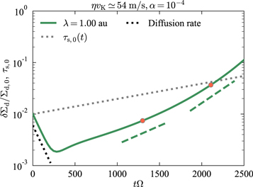
Figure 2. Results of the local simulation with λ = 1 au, Σd ,0/Σg ,0 = 10−3, and α = 10−4. The green solid line shows the amplitude of the dust surface density perturbation as a function of tΩ. The gray dotted line shows the time evolution of the background stopping time τs,0. The initial dust surface density perturbation is damped by the diffusion at a rate of Dk2 (black dotted line). The perturbation exponentially grows after the initial damping. The green dashed lines show the growth rates derived in the previous linear analyses (Equation (18)). We use physical values at times marked by the orange filled circles to derive the growth rate. The linear analyses are in good agreement with the simulation at each point.
Download figure:
Standard image High-resolution imageFigure 3 shows the time evolution of δΣd/Σd
,0 and δτs,0/τs,0 as a function of the radial position and time. As predicted by Tominaga et al. (2021), the dust size perturbation is shifted outward relative to the surface density perturbation (see Section 2.2 of Tominaga et al. 2021). Note that the dust cells move at the perturbed velocity δ
vx
, and we extracted the background drift motion  (Equations (20) and (21)). Therefore, the inward radial propagation of the perturbations in Figure 3 means that the phase speed is larger than the background drift speed, which is also consistent with the results in Tominaga et al. (2021) (see also Equation (18)).
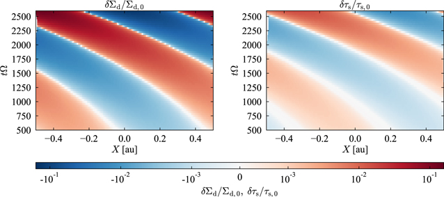
Figure 3. Growth and propagation of δΣd/Σd ,0 (left panel) and δτs,0/τs,0 (right panel) obtained from the local simulation with λ = 1 au and α = 10−4. Note that the horizontal axis is the radial position X in the background-dust-rest frame (Equation (22)). The phase shift between δΣd and δτs and the radial propagation of the perturbations are consistent with the previous linear analyses (Tominaga et al. 2021).
Download figure:
Standard image High-resolution imageFigure 4 compares the results of simulations for three different wavelengths: λ = 0.25, 1, and 4 au. Shorter-wavelength perturbations experience more significant initial damping due to the diffusion (e.g., the blue solid line). At a later time, each simulation shows exponential growth consistent with the previous linear analyses (see dashed lines), which in turn validates our numerical scheme.
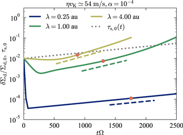
Figure 4. Results of the local simulation with α = 10−4 for λ = 0.25, 1, and 4 au. The blue, green, and yellow solid lines show the evolution of δΣd/Σd ,0 for each wavelength. The gray dotted line shows the time evolution of the background stopping time τs,0. The blue, green, and yellow dashed lines show the growth rates derived in the previous linear analyses (Equation (18)). We use physical values at times marked by the orange filled circles to derive the growth rate. The linear analyses have a good agreement with each simulation.
Download figure:
Standard image High-resolution imageWe note that the linear analyses ignored the background evolution of the stopping time. Regardless of this assumption, the growth rates from the linear analyses well reproduce the exponential growth rates observed in the local simulations. This in turn validates the assumption in the linear analyses.
4. Radially Global Simulations
In this section, we show results of radially global simulations. We investigate (1) whether the instability develops into the nonlinear growth phase before dust grains fall onto a central star, and τs locally increases up to unity, and (2) how much dust surface density and dust-to-gas ratio increase.
4.1. Disk Models
We assume the following gas surface density and temperature profile:


where Σg ,10, q, and T100 are constant parameters. We assume an initial dust-to-gas ratio of 10−2 in all runs:

Initial dust size is assumed to be 10 μm. The choice of the initial dust sizes insignificantly affects background evolution unless the dimensionless stopping time is much less than unity because dust grains initially just grow in size at the initial location.
The parameter q on the exponent of the surface density profile takes three different values: q = 1, 2, and 3. In most runs, we set  . We adopt smaller Σg
,10 for q = 1 so that the gas disks are stable to nonaxisymmetric GI in the domain: Q ≡ csΩ/πGΣg > 2.
. We adopt smaller Σg
,10 for q = 1 so that the gas disks are stable to nonaxisymmetric GI in the domain: Q ≡ csΩ/πGΣg > 2.
We next set up initial perturbations. As in the local simulations (Section 3), we displace the cells and input perturbations only in dust surface density at t = 0. The displacement δ ξ adopted in the radially global simulations is the following (see Figure 1):

where ξ0 = 0.2(rout − rin)/N, rout is the outer boundary radius, and ϕj is a random number less than unity. As described below, we adopt the radial domain size of 95 au in most runs with N = 214 = 16,384. Thus, the 128th mode included in δ ξ has a wavelength less than 1 au. The above displacement gives initial Σd-perturbations of about 10%–20% at most, but dust diffusion decreases the perturbation amplitudes down to 1% or a few percent before the onset of coagulation instability. We note that the adopted δ ξ in the present simulations is small enough that cell crossing by the initial displacement does not occur.
To see wave propagation during the development of the instability, we input initial perturbations only in the outer half region, reducing the displacement δ ξ in all runs as follows:

where R0 = 50 au and Δr = 1 au. If we input perturbations without the reduction, we observe fast growth of coagulation instability at inner radii and dust growth up to τs = 1 well before outer dust grains start drifting because the timescales of the instability are proportional to Ω−1 ∝ r3/2 (see also Appendix B).
Labels of runs, parameters, the adopted initial perturbation are listed in Table 1.
Table 1. Summary of Parameters and Results
| Runs | q |

| T100 (K) | α | rin (au) | τs → 1 via CI? | (rring, Σd ,ring/Σg) |
|---|---|---|---|---|---|---|---|
| q3T28a1 | 3 | 1 | 28 | 1 × 10⁻⁴ | 5 | Yes | (34.9 au, 2.80 × 10⁻¹) |
| q3T20a1 | 3 | 1 | 20 | 1 × 10⁻⁴ | 5 | Yes | (37.7 au, 2.96 × 10⁻¹) |
| q3T10a1 | 3 | 1 | 10 | 1 × 10⁻⁴ | 5 | Yes | (40.1 au, 1.65 × 10⁻¹) |
| q2T28a1 | 2 | 1 | 28 | 1 × 10⁻⁴ | 5 | Yes | (31.5 au, 1.67 × 10⁻¹) |
| q2T20a1 | 2 | 1 | 20 | 1 × 10⁻⁴ | 5 | Yes | (32.4 au, 1.50 × 10⁻¹) |
| q2T10a1 | 2 | 1 | 10 | 1 × 10⁻⁴ | 5 | Yes | (39.7 au, 1.23 × 10⁻¹) |
| q1T28a1* | 1 | 0.5 | 28 | 1 × 10⁻⁴ | 20 | Yes | (30.3 au, 1.48 × 10⁻¹) |
| q1T20a1* | 1 | 0.5 | 20 | 1 × 10⁻⁴ | 20 | Yes | (33.9 au, 1.40 × 10⁻¹) |
| q1T10a1* | 1 | 0.5 | 10 | 1 × 10⁻⁴ | 20 | Yes | (33.6 au, 5.42 × 10⁻²) |
| q3T20a3 | 3 | 1 | 20 | 3 × 10⁻⁴ | 5 | Yes | (13.6 au, 1.00 × 10⁻¹) |
| q3T20a5 | 3 | 1 | 20 | 5 × 10⁻⁴ | 5 | Yes | (6.74 au, 7.25 × 10⁻²) |
| q2T20a3 | 2 | 1 | 20 | 3 × 10⁻⁴ | 5 | Yes | (16.4 au, 7.50 × 10⁻²) |
| q2T20a5 | 2 | 1 | 20 | 5 × 10⁻⁴ | 5 | Yes | (9.22 au, 6.24 × 10⁻²) |
| q1T20a1 | 1 | 0.5 | 20 | 1 × 10⁻⁴ | 5 | Yes | (27.3 au, 9.70 × 10⁻²) |
| q1T20a3 | 1 | 0.5 | 20 | 3 × 10⁻⁴ | 5 | Yes | (8.72 au, 1.22 × 10⁻²) |
| q1T20a5 | 1 | 0.5 | 20 | 5 × 10⁻⁴ | 5 | Yes | (7.15 au, 8.99 × 10⁻³) |
| q1T20a3* | 1 | 0.5 | 20 | 3 × 10⁻⁴ | 20 | No | ⋯ |
| q1T20a5* | 1 | 0.5 | 20 | 5 × 10⁻⁴ | 20 | No | ⋯ |
Note. "CI" at the top of the seventh column stands for coagulation instability. The dust-to-gas ratio at the resulting rings (eighth column) is derived from the last time step of each simulation.
Download table as: ASCIITypeset image
4.2. Numerical Setups
The number of cells N is 214 = 16,384. The domain is uniformly spaced by N cells at t = 0. The main reason to adopt this large number of cells is that the nonlinear evolution of the instability results in very narrow structures whose width is less than 0.1 au as shown in the next subsection. Note that the Lagrangian scheme automatically increases the spatial resolutions of high-density regions. However, coagulation instability develops after dust grains are depleted as a result of the radial drift, meaning that the resolution of the background state first becomes lower than the initial resolution. Therefore, to describe nonlinear coagulation instability, we need the relatively large number of cells even when we utilize the Lagrangian scheme. We note again that the Lagrangian scheme is free from numerical diffusion regardless of the number of cells, and thus this is still the advantage of using the Lagrangian scheme.
The inner and outer boundaries are set initially at rin = 5 au and rout = 100 au in most runs. As a disk evolves and dust grows, the cells move inward and flow out of the domain. We thus let the inner boundary move with the first cell boundary while the outer boundary radius is fixed. We discuss disk evolution in rin(t = 0) ≤ r ≤ rout.
We adopt rin = 20 au at t = 0 for a run with T100 = 10 K and q = 1 because even background dust evolution results in dust sizes of τs = 1 at inner radii (q1T10a1* run). We also adopt rin = 20 au in other runs to investigate parameter dependence under the same configuration of the domain (the q1T28a1* and q1T20a1* runs) and to check the rin-dependence of the results (the q1T20a3* and q1T20a5* runs).
The moment method we utilize in this work might be valid for τs ≤ 1 because dust grains of τs = 1 are the most significantly depleted because of the fastest drift speed, and dust size distribution will become bimodal if there are larger solids of τs > 1. Therefore, we stop simulations once the dimensionless stopping time becomes larger than unity as a result of coagulation instability. The simulations otherwise last for 2 × 10⁵ yr.
4.3. Results
The results are briefly summarized in the seventh and eighth columns of Table 1. In the eighth column, we list radial locations of dust surface density maximum, rring, and resulting dust-to-gas ratios, Σd ,ring/Σg, at the time when τs = 1 is achieved. We find that in most runs coagulation instability develops into the nonlinear growth phase before perturbations drift into the outside of the domain, locally increasing τs up to unity. We also find that dust-to-gas surface density ratio can increase at least by an order of magnitude after dust depletion down to Σd/Σg ∼ 10−3.
Figure 5 shows the results of the q2T20a1 run. The left two panels show the time evolution of dust surface density and dimensionless stopping time. We also show the evolution in the absence of the initial perturbation in the right two panels. As mentioned in the previous studies, inside-out dust coagulation and radial drift result in dust depletion and dust-to-gas ratio of order 10−3 (e.g., Brauer et al. 2008). In the presence of the initial perturbations, they exponentially grow via coagulation instability, and dust-to-gas ratio locally increases up to ∼10−1. The dimensionless stopping time increases above unity around the most collapsed dust ring at t = 9.0 × 10⁴ yr.
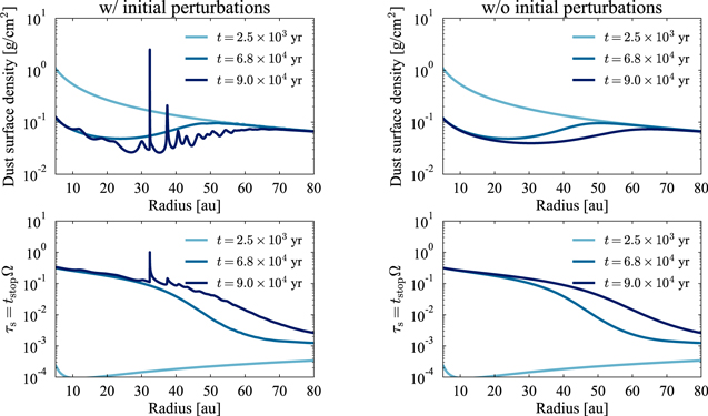
Figure 5. Time evolution of dust surface density (top panels) and dimensionless stopping time (bottom panels) obtained from the q2T20a1 run. The left two panels and the right two panels show evolution with and without initial perturbations, respectively. Coagulation instability locally increases dust-to-gas ratio up to ∼10−1. We stop the simulation at t = 9.0 × 10⁴ yr since the dimensionless stopping time τs becomes larger than unity around the most collapsed dust ring.
Download figure:
Standard image High-resolution imageRegardless of the presence of the radial dust diffusion, we find that the nonlinear coagulation instability creates narrow rings. This is because the radial concentration is driven by the radial drift velocity ∼ τs η vK, which is much larger than D/r by a factor of τs/α. The difference in the drift velocity can increase the dust surface density significantly until the density gradient ∂Σd/∂r becomes large enough that the dust diffusion balances with the drift motion.
Figure 6 shows dust surface density, dust sizes, and radial velocity profiles around the most collapsed ring in the q2T20a1 run. Dust sizes are 1–10 cm within the ring in this run. We note that very narrow ring structures with widths of ∼0.05 au are well resolved in our simulations. The bottom panel of Figure 6 shows that there is a radial gradient in vr in 32.30 au ≲ r ≲ 32.35 au, while vr is almost uniform around the Σd-peak radius (the dashed line). Similar velocity profiles are found in other runs. This indicates that the ring will sweep inner dust grains up while moving inward, and the dust surface density in the ring will increase through further evolution until significant dust growth results in τs ≫ 1 and quenches the dust drift. Figure 5 shows that there are also some rings that are still growing at r ≳ 37 au. Therefore, it is expected that further evolution will lead to dust retention at multiple locations with τs ≥ 1.
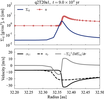
Figure 6. Radial profile of Σd and dust size a (top panel), and radial velocities  ,
,  , and
, and  (bottom panel) around the most collapsed ring at the final time step. Red filled circles show the position of the cell boundaries. One can see that the ring structure is well resolved even though the radial width is less than 0.1 au. We find the radial gradient in vr
around the left-side tail of the Σd profile (32.3 au ≲ r ≲ 32.35 au), while vr
is almost uniform within the ring. Thus, the ring will sweep inner dust grains up, and the surface density increases through further evolution.
(bottom panel) around the most collapsed ring at the final time step. Red filled circles show the position of the cell boundaries. One can see that the ring structure is well resolved even though the radial width is less than 0.1 au. We find the radial gradient in vr
around the left-side tail of the Σd profile (32.3 au ≲ r ≲ 32.35 au), while vr
is almost uniform within the ring. Thus, the ring will sweep inner dust grains up, and the surface density increases through further evolution.
Download figure:
Standard image High-resolution imageFigure 7 shows results of the q2T20a5 run. Diffusion with larger α quenches short-wavelength modes that will exponentially grow for smaller α. Nevertheless, coagulation instability locally increases τs up to unity as well as in the q2T20a1 run. The most collapsed ring in the q2T20a5 run is located at smaller radii than in the q2T20a1 run. The reason for this is smaller growth rates of coagulation instability in the q2T20a5 run because of stronger turbulent diffusion. Indeed, in smaller-domain-size simulations (q1T20a3* and q1T20a5*) perturbations flow out across r = rin(t = 0) before a significant increase in their amplitudes. One can see that dust grains initially located at the perturbed region drift into smaller radii in Figure 8. Figure 8 shows the time evolution of cumulative mass profiles for the q2T20a1 and q2T20a5 runs. The cumulative mass also includes the mass of cells flowing out of the domain. Because of the mass conservation, one can see the motion of cells from Figure 8. For instance, a dust cell initially at r = 50 au is located at intersections of the black dashed line and each cumulative mass profile. We also plot a line that shows the cumulative mass of M(<49 au) at t = 0 yr (gray dashed line) as a reference. The positions of the dust rings in each run correspond to positions of "cliffs" on the cumulative mass profiles. The rings in both runs consist of dust cells initially located around r ≃ 49–50 au. We thus attribute the difference in rring to the difference in radial distance over which dust drifts within the growth time of coagulation instability. 4 This interpretation is consistent with our previous linear analysis that shows that the phase velocity is roughly given by the dust drift velocity.

Figure 7. Time evolution of dust surface density (left panel) and dimensionless stopping time (right panel) obtained from the q2T20a5 run. As in the q2T20a1 run, we observe a local increase in dust-to-gas ratio by an order of magnitude. The dimensionless stopping time locally becomes larger than unity at t = 8.7 × 10⁴ yr.
Download figure:
Standard image High-resolution image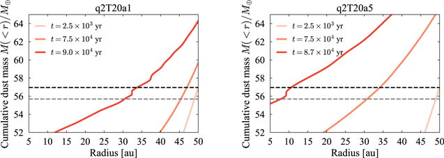
Figure 8. Cumulative dust mass profile from the q2T20a1 run (left panel) and the q2T20a5 run (right panel). The ring locations rring correspond to "cliffs" in the cumulative mass profiles. The gray dashed line and the black dashed line show M(<49 au) and M(<50 au) at t = 0 yr, respectively. One can see that the resulting dust rings in both runs consist of dust cells initially located around 50 au.
Download figure:
Standard image High-resolution imageWe investigate η vK-dependence of the ring position and resulting dust-to-gas ratio by changing T100 for a given q and α = 1 × 10⁻⁴. Figure 9 summarizes the results (solid lines with marks). In the left panel, the shaded regions show the final positions of dust cells that are initially located at 49 au ≤ r ≤ 50 au. All marks are in the shaded regions. This means that perturbations initially located around the inner edge of the perturbed region (r ≃ 50 au) have enough time to develop via coagulation instability toward the nonlinear phase; the ring would consist of dust cells initially located at r ≫ 50 au if the growth timescale was much longer than the drift timescale. We find that when q is fixed the radial position rring decreases as η vK. Since the shaded regions show the similar trend, we attribute the η vK-dependence seen for a given q to the difference in the drift velocity: dust grains with a certain τs have faster drift speed for larger η vK and reach inner regions.

Figure 9. Dependence of rring (left panel) and Σd ,ring/Σg (right panel) on η vK. In both panels, solid lines with marks show the resulting rring and Σd ,ring/Σg. In the left panel, we plot the radial location of dust cells that are initially located in 49 au ≤ r ≤ 50 au with the shaded regions. We find that larger η vK makes the ring radius smaller. This is because dust grains with a certain τs move faster for larger η vK.
Download figure:
Standard image High-resolution imageThe left panel of Figure 9 also shows that in most cases rring is smaller for smaller q, although smaller-q runs show lower values of η vK (see dark-blue and orange lines). This trend originates from the radial profile of the background τs. Figure 10 shows the radial profile of τs in the q1T20a1 and q3T20a1 runs. At the final time step (dark-blue lines), background τs reaches the drift-limited value at inner radii. The q1T20a1 run shows r-dependent background τs, while the q3T20a1 run shows almost uniform background τs. The background τs thus becomes larger in the q1T20a1 run than in the q3T20a1 run, meaning that the drift velocity proportional to τs η vK can become larger for q = 1 even though η vK is smaller. Therefore, dust grains and perturbations move inward more efficiently for smaller q, which explains q-dependence in Figure 9.

Figure 10. Radial profiles of τs in the q1T20a1 run (left panel) and the q3T20a1 run (right panel). In each run, τs reaches unity in the most collapsed ring at t = 9.6 × 10⁴ yr and 6.1 × 10⁴ yr, respectively. The background τs increases as r decreases in the q1T20a1 run and becomes larger than the background τs in the q3T20a1 run. This means that dust grains drift inward more efficiently in the former run, which explains the trend that rring is smaller for smaller q.
Download figure:
Standard image High-resolution imageThe resulting Σd ,ring/Σg is almost similar in all runs, although we can see slightly larger values for larger η vK and larger q. This slight dependence is also explained based on the difference in the τs profile as in the q-dependence in the left panel. 5 Larger η vK reduces the background drift-limited τs because of the higher drift speed. In such a case, coagulation instability locally increases dust surface density more before τs in rings reaches unity via the instability and we stop the simulations. If q is small, the background τs becomes larger especially at inner radii as mentioned above, and there is little space for τs perturbations to develop up to unity, leading to smaller dust surface density.
5. Discussions
5.1. On Possible Ways to Retain Dust Grains in a Disk
As shown above, we observe significant dust concentration into a ring via coagulation instability. There are some rings that are growing toward the nonlinear phase (see Figure 5). The radial drift of the rings halts as a result of further dust growth beyond τs = 1. On the other hand, remaining dust grains in gaps and other less dense regions still suffer from the radial drift toward the central star. For retaining such dust grains in the disk, either of the following two processes will be necessary: (A) coagulation instability of the remaining dust grains operates and triggers concentration into second-generation rings, or (B) the first-generation rings catch the remaining dust that radially drifts through the ring.
Process (A) will be expected since any disturbances on a disk give rise to seed perturbations; in the present simulations, we input seed perturbations only at t = 0 yr. If dust grains in the first-generation rings significantly grow in size (τs ≫ 1), coagulation instability of the remaining dust grains might be insensitive to the rings. Therefore, successive development of coagulation instability will play the key role in retaining dust grains in a disk.
Next, we discuss the efficiency of process (B). We evaluate collisional "optical depth" regarding a collision between a drifting dust grain and dust grains in the first-generation ring. The associated mean free path of a drifting dust at the midplane in a ring, l, is given by

where aring and adrift are the sizes of the dust in a ring and the drifting dust, respectively, and  . We assume
  and the Epstein law, and thus τs,ring/τs,drift = aring/adrift in the ring. For a ring width of ΔRring, collisional "optical depth," τcoll, is
  , and thus
The value of ΔRring/H is roughly given by the value of the most collapsed ring in the q2T20a1 run: ΔRring ∼ 0.05 au and H ≃ 2.17 au at r ≃ 32.3 au. The value of τs,drift/τs,ring in the last parentheses in the second row of Equation (30) is less than unity, and thus we can neglect it. The last factor comes from  and is less than 10 for τs,drift = 0.1 ≪ τs,ring. We then obtain τcoll < 1. The collisional optical depth can be much larger than unity only in a special case where the ring and the drifting dust have a similar radial velocity, i.e.,
  . This is not our main focus of this discussion since we consider dust grains that have radial relative velocity and drift with respect to the ring. In the limit of τs,ring ≫ 1, the last factor converges to ∼ 0.5/τs,drift ∼ 5 for τs,drift = 0.1. In such a limit, we obtain τcoll ≪ 1 because of the τs,ring-dependence appearing in the second row of Equation (30). In this way, Equation (30) indicates that the dust in the ring and the drifting dust are collisionless, i.e., the drifting dust grains can pass through the ring, especially after dust growth proceeds and τs,ring becomes larger than unity. Therefore, we expect that process (B) is inefficient in the present case.
As described above, process (A) is more important to retain dust grains in a disk. Note that Equation (30) validates the hypothesis of process (A) since it will occur when remaining dust grains are insensitive to large grains in the rings. For the further discussion, we need simulations with full-size distributions or at least two-population simulations that can treat drifting dust and large solids (e.g., Dra̧żkowska & Alibert2017). This will be addressed in our future studies.
5.2. Comments on the Development to Secular GI
Our previous work proposed a scenario in which if coagulation instability operates in a disk, the instability is expected to set up preferable locations for secular GI to develop toward planetesimal formation. In this work, we demonstrate that coagulation instability operates indeed during the inside-out dust evolution. Those results support our scenario. As shown in Appendix C, the rings observed in the present simulations can be unstable to secular GI if they form in outer regions where Toomre's Q is relatively small, for example, Q ≲ 10. Weaker turbulence is also required as shown in the previous studies on secular GI (e.g., Shariff & Cuzzi 2011; Youdin 2011; Takahashi & Inutsuka 2014; Tominaga et al.2019).
Although the present simulations demonstrate the possible path toward planetesimal formation, we have to treat the back-reaction for rigorous discussions. The effect of the back-reaction is expected to be insignificant in the linear growth phase. This is because coagulation instability starts to grow after dust density decreases and dust-to-gas surface density ratio becomes on the order of 10−3. On the other hand, the back-reaction will become significant in the nonlinear growth phase, which will limit the maximum dust density in rings. We give further discussion on the development to secular GI in Paper II, where we present simulations with not only the back-reaction but also fragmentation.
6. Summary
Formation of planetesimals has been widely studied but is still under debate. In the case of outer planetesimal formation, disk instabilities have been proposed as a possible mechanism. In particular, some studies indicate that planetesimal formation via GI subsequent to streaming instability may explain the origin of Kuiper Belt objects (e.g., McKinnon et al. 2020). However, the viability of such instabilities is still under debate because even weak turbulence (α ∼ 10−5) can suppress streaming instability (e.g., McNally et al. 2021).
Our previous study (Tominaga et al. 2021) proposed a new instability named coagulation instability, which is expected to trigger dust concentration and to assist planetesimal formation in a protoplanetary disk. Coagulation instability develops even in the presence of turbulence of α ∼ 10−4.
In this work (Paper I), we perform numerical simulations and prove that coagulation instability operates during the inside-out evolution via dust growth and even for the background dust-to-gas ratio of ∼10−3. The development of coagulation instability causes radial dust concentration into rings against the dust depletion due to the radial drift. Nonlinear growth also increases τs up to unity in the rings even at outer radii (>10 au), showing the possible path of dust growth beyond the drift barrier. We intentionally exclude the back-reaction and simplify the simulations to isolate the contribution to the dust concentration. The simplified simulations demonstrate that the back-reaction is not prerequisite for the dust concentration via coagulation instability, which is in contrast to the self-induced dust trap (Gonzalez et al. 2017).
We measure the enhanced dust-to-gas ratio in the most collapsed ring at the time when the dimensionless stopping time τs becomes unity via coagulation instability. We find that the dust-to-gas ratio increases by an order of magnitude or more and that the ratio can reach ∼0.1 in the present simulations without back-reaction. The resulting dust-to-gas ratio Σd ,ring/Σg at the final time step is only slightly higher in a disk with larger η vK (Figure 9). This is because background evolution leads to smaller τs (drift-limited), and coagulation instability increases dust density more until τs = 1 is achieved.
We also find that stronger turbulence slows the growth of coagulation instability, and as a result, rings form at inner radii as α increases (Table 1 and Figure 8). Too large α prevents coagulation instability from developing and creating dense rings before perturbations flow out of the numerical domain.
We discuss the further development of resulting rings and dust grains in Section 5. There are two possible ways to retain dust grains after the formation of the first-generation rings: (A) coagulation instability of the remaining dust grains operates and forms next-generation rings, or (B) the first-generation rings catch the remaining dust. We expect that process (A) is more important for the dust retention. Process (B) is insignificant, and dust grains coming from the outer region will pass though the ring without collisions once dust grains in the rings become large enough (τs,ring ≫ 1; see Equation (30)).
Tominaga et al. (2021) proposed a scenario in which a combination of coagulation instability and secular GI will explain planetesimal formation. The results of the present simulations support this scenario. As briefly mentioned in Section 5.2, the radial concentration observed in the present simulations will be the key to trigger secular GI in a disk (see also Appendix C). Further discussion is given in Paper II.
In this paper, we neglect the effects of back-reaction and dust fragmentation to isolate the contributions to dust growth and concentration. The simulations under this assumption are worth being presented since this simplification allows clear distinction between coagulation instability and the self-induced dust trap proposed in Gonzalez et al. (2017): the back-reaction is not a prerequisite for the local dust concentration via coagulation instability. We expect that a combined process of coagulation instability and the self-induced dust trap is one promising mechanism to save dust grains (see discussion in Paper II). Linear growth phase is insignificantly affected by the back-reaction since coagulation instability starts to grow after dust-to-gas ratio decreases (∼10−3). On the other hand, nonlinear growth of coagulation instability will be affected by the back-reaction. The back-reaction decelerates the radial drift and makes it easier for dust grains to overcome the drift barrier in rings before Σd/Σg increases significantly. Besides, the linear growth rate is reduced by fragmentation according to the linear analysis in Tominaga et al. (2021). In Paper II, we present results of simulations where the effects of the back-reaction (the drift deceleration) and the fragmentation are taken into account.
We thank Hidekazu Tanaka, Takeru K. Suzuki, Sanemichi Z. Takahashi, and Elijah Mullens for fruitful discussions and helpful comments. We also thank the anonymous referee for the review, which helped us to improve the manuscript. This work was supported by JSPS KAKENHI grant Nos. JP18J20360, 21K20385 (R.T.T.), 16H02160, 18H05436, 18H05437 (S.I.), 17H01103, 17K05632, 17H01105, 18H05438, 18H05436, 20H04612, 22H00179, 22H01278, and 21K03642 (H.K.). R.T.T. is also supported by the RIKEN Special Postdoctoral Researchers Program.
Appendix A: Local Simulations for Weaker Turbulence
Figure 11 shows results of the local simulations with α = 10−5. We perform three runs with three different wavelengths: λ = 0.25, 1, and 4 au. As in the case of α = 10−4, we find a good agreement between the previous linear analyses and the local simulations. The perturbations grow faster than in the simulations with α = 10−4 because the diffusion is ineffective. The ratio of the growth rates and the coagulation rate (see the gray dotted line) is also larger. Thus, coagulation instability more quickly develops at shorter spatial scales in more weakly turbulent disks than assumed in Section 4, leading to dust growth beyond the drift barrier.
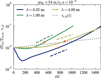
Figure 11. Results of the local simulation with α = 10−5 for λ = 0.25, 1, and 4 au. The blue, green, and yellow solid lines show the evolution of δΣd/Σd ,0 for each wavelength. The gray dotted line shows the time evolution of the background stopping time τs,0. The blue, green, and yellow dashed lines show the growth rates derived in the previous linear analyses (Equation (18)). We use physical values at times marked by the orange filled circles to derive the growth rate. The linear analyses have a good agreement with each simulation.
Download figure:
Standard image High-resolution imageAppendix B: Critical Radius for Coagulation Instability to Save Dust Grains
In the present simulations, we input initial perturbations only in the outer half region and observe that the perturbations can grow before they flow out of the numerical domain in most runs. This process helps dust grains to avoid radial drift and depletion. In this appendix, we roughly estimate a "critical radius" that is a boundary dividing the radial regions where coagulation instability can save dust grains or not.
The necessary condition for the instability to save dust grains is that the radial drift timescale is longer than the growth timescale of coagulation instability. Similar discussion is given in Section 4.4 in Tominaga et al. (2021). We here focus on the critical radius at which the ratio of the above two timescales is unity, while we focused on τs- and ε-dependences of the ratio in the previous study. Following the notation in Tominaga et al. (2021), we denote the radial drift timescale by ttravel, which is given by

For simplicity, we assume ∣vr ∣ ≃ 2τs,0 η vK. The necessary condition to save dust is ttravel > n−1, which yields

Note that the growth rate has τs,0- and η vK-dependences. Roughly speaking, we can expect the growth rate to be proportional to the square root of those physical quantities. Thus, as a net dependence, the critical radius given the right-hand side of Equation (B2) depends roughly on the square root of τs,0 and η vK. We also note that the growth rate also depends on α and ε (see Tominaga et al. 2021).
Equation (B2) states that dust grains initially located at r ≃ 10 au are potentially saved by coagulation instability. The adopted value of n in Equation (B2) is about the maximum growth rate for τs,0 = 0.1, α = 1 × 10⁻⁴, and ε = 1 × 10⁻³ in the MMSN disk (see, e.g., Figure 8 in Tominaga et al. 2021). According to the results of the radial global simulations, coagulation instability already operates when ε becomes just a few times lower than the initial value (0.01). In such cases, the growth rate is larger than the above value according to the linear analyses in Tominaga et al. (2021), and the critical radius will decrease. On the other hand, the critical radius becomes larger if the radial diffusion is stronger since the growth rate decreases.
Note that perturbations that start growing at inner radii have larger growth rates since the growth rate is scaled by Ω ∝ r−3/2, and thus the critical radius for such inner perturbations is smaller. For example, the critical radius is about 3.8 au for n = 3 × 10⁻³ Ω (10 au), τs,0 = 0.1, and η vK = 54 m s−1. In this case, inner dust grains will be saved as the inner perturbations grow via the instability.
Finally, we also note that Equation (B2) is the necessary condition. If the initial amplitudes of perturbations are small, it takes multiple growth timescales for coagulation instability to concentrate dust grains significantly. In such a case, the critical radius is larger than shown in Equation (B2).
Appendix C: Secular Gravitational Instability in Resulting Dust Dense Regions
The radial dust concentration shown in the present simulations is the possible connection to planetesimal formation via secular GI (e.g., Ward 2000; Youdin 2005a, 2005b, 2011; Michikoshi & Kokubo 2012; Takahashi & Inutsuka 2014, 2016; Tominaga et al. 2018, 2019, 2020; Pierens 2021). Although the back-reaction should be taken into account in the simulations for more rigorous discussion (Section 5.2), it is still worth noting whether secular GI is operational in the rings observed in the present simulations without the back-reaction. In this appendix, we thus briefly examine the stability of the rings.
Growth efficiency of secular GI is determined by four parameters: dust-to-gas ratio, dimensionless stopping time, turbulence strength, and Toomre's Q value for gas. A condition for the growth of secular GI is given as follows (Tominaga et al. 2019) 6 :
where  and
and  is velocity dispersion of dust grains (see also Youdin 2005a; Youdin & Lithwick 2007). We briefly describe the physical insight into the growth condition of secular GI below. For
  and
and  , Equation (C1) is reduced as follows (see also Equation (21) in Takahashi & Inutsuka 2014):

This simplified equation clearly represents the key physical conditions for the onset of secular GI. The parameter Qgd is a measure of how massive the dusty gas disk is. The other parameter Qdrag is a ratio of two timescales: (1) diffusion time over a spatial scale of H, and (2) a timescale for which dust moves over a distance H at the terminal velocity tstop πGΣd. Secular GI can grow in a self-gravitationally stable disk with Qgd > 1 when the dust diffusion is weak: Qdrag < 1 is necessary. Note that the diffusion coefficient D in the linear analyses of secular GI is related to the radial diffusion. If the vertical diffusivity is also given by D, we obtain another form of the parameter Qdrag as follows:
where  is the midplane dust density, and we also adopt
  (e.g., Youdin & Lithwick 2007). If we neglect the factor difference, the numerator of the first term, Ω2/G, roughly corresponds to the Roche-like density that determines the stability of three-dimensional mode in a self-gravitating disk (see, e.g., Goldreich & Lynden-Bell 1965a; Sekiya 1983). We can see that the above necessary condition Qdrag < 1 can be satisfied even for ρd ≲ Ω2/G since the dust layer is much thinner (Hd/H ≪ 1) for grown dust grains. Therefore, secular GI does not require a gravitationally unstable dust layer for its onset, in contrast to the classical GI.
We include cd in the following discussion, although our simulations do not include the effect of the velocity dispersion in the equation of motion for dust. Neglecting cd in Equation (C1) makes 1 − F slightly larger, and a ring appears more unstable to secular GI.
Figure 12 shows dust surface density profiles at the final time steps from the six runs. We overplot filled circles whose color shows whether the condition for secular GI is satisfied at the dust cells or not. Secular GI is operational at red regions where 1 − F is positive (Equation (C1)). In some runs, we find that secular GI becomes unstable at the dust rings.

Figure 12. Dust surface density profiles around the most collapsed ring in the six runs. We plot filled circles at the cell positions, with color showing the condition for secular GI (see Equation (C1)). Secular GI can operate for 1 − F > 0.
Download figure:
Standard image High-resolution imageThe rings forming at outer radii can be sufficiently unstable to secular GI, while inner rings tend to be stable or marginally unstable even when Σd increases by an order of magnitude (see, e.g., the panels of the q2T20a5 and q2T20a1 runs). This is partly due to the difference in the turbulence strength α. Dust diffusion with larger α stabilizes secular GI. Thus, less turbulent disks are still preferable even when dust surface density is increased by coagulation instability. Toomre's Q value of the background gas disk also significantly affects the stability of the rings. From the definition of Toomre's Q, we have
for T ∝ r−1/2, Ω ∝ r−3/2, and Σg ∝ r−q/2, meaning that Q increases as r decreases for q = 1, 2, and 3. As already mentioned in the previous studies, secular GI grows more easily for smaller Q (see, e.g., Youdin 2005a, 2011; Takahashi & Inutsuka 2014; Tominaga et al. 2019), although Q < 1 is not required. In other words, secular GI becomes operational more easily at outer radii, and thus in outer rings. Note that secular GI is stable at dust-depleted regions (blue regions in Figure 12). Thus, coagulation instability and resulting dust concentration are important for the onset of secular GI.
Appendix D: On the Effect of Porosity of Dust Aggregates
Although we assume the spherical compact dust in the present simulations, dust collisions will produce porous aggregates (e.g., Dominik & Tielens 1997; Suyama et al. 2008; Wada et al. 2008). It is known that the coagulation timescale becomes shorter for such porous dust aggregation (e.g., Okuzumi et al. 2012; Kobayashi & Tanaka 2021). The difference in the timescales can be estimated by introducing a filling factor f ≡ ρbulk/ρmon, where ρbulk and ρmon are the mass densities of a single aggregate and a single monomer, respectively (see, e.g., Kataoka et al. 2013, 2014). As noted in the previous studies, the coagulation timescale is proportional to the mass-to-area ratio (see, e.g., Section 4 of Okuzumi et al. 2012):
(see also Equation (8)). Here we assume that the mass of a single porous aggregate is given by 4π ρbulk a3/3. 7 Thus, the coagulation timescale is f times shorter than in the case of a compact dust.
As found in Tominaga et al. (2021) and reviewed in Section 3.1, the growth timescale of coagulation instability is scaled by the coagulation timescale. Thus, coagulation instability operates even when we consider the porosity. In the porous dust case, we expect that (1) the growth is faster and (2) the most unstable wavelength becomes shorter since the wavelength is scaled by the growth-drift length  (Tominaga et al. 2021). We note that the stopping time is also proportional to mp/π
a2, and thus the growth-drift length is proportional to f2.
(Tominaga et al. 2021). We note that the stopping time is also proportional to mp/π
a2, and thus the growth-drift length is proportional to f2.
According to the previous studies (Okuzumi et al. 2012; Kobayashi & Tanaka 2021), even porous aggregation is faced with the fast radial drift at r > 10 au, while dust at r ≤ 10 au quickly grows to planetesimals. Thus, such an outer region will be a place where coagulation instability significantly affects the dust evolution.
Footnotes
- 3
Although the Lagrangian-cell method developed in Tominaga et al. (2018) is used with a symplectic integrator in our previous studies, we adopt the Runge–Kutta method in this work because we assume the terminal velocity for dust instead of solving equations of motion.
- 4
The background evolution in the q2T20a5 run is slightly faster than in the q2T20a1 run when dust grains are small and α > τs. We find that the difference in the dust scale height leads to the difference in the dust growth time in such a case. Note that when dust grains become large (α ≫ τs) and we can approximate the dust scale height as
 , the coagulation timescale is hardly dependent on α (see also Brauer et al. 2008; Okuzumi et al. 2012; Sato et al. 2016). In particular, the coagulation timescale is independent of α for the turbulence-driven coagulation ().
 - 5
The difference in initial perturbations will also cause a slight difference in the dust-to-gas ratio to some extent.
- 6
We use the dust-to-gas surface density ratio to discuss the growth condition of secular GI, although the dust-to-gas ratio around the dust sublayer might be more important. We do not discuss the effect of vertical structure in the context of secular GI because linear growth of secular GI on the r − z plane has not been studied and is beyond the scope of this paper.
- 7
As mentioned in Okuzumi et al. (2012), the early stage of porous aggregation in a disk leads to aggregates whose fractal dimension is ≃2. However, this stage will be irrelevant to coagulation instability. This is because the dimensionless stopping time of such aggregates is comparable to those of monomers and is too small, and they hardly drift.
