


Abstract
The cosmographic approach, a Taylor expansion of the Hubble function, has been used as a model-independent method to investigate the evolution of the universe in the presence of cosmological data. Apart from possible technical problems like the radius of convergence, there is an ongoing debate about the tensions that appear when one investigates some high-redshift cosmological data. In this work, we consider two common data sets, namely, Type Ia supernovae (Pantheon sample) and the Hubble data, to investigate advantages and disadvantages of the cosmographic approach. To do this, we obtain the evolution of cosmographic functions using the cosmographic method, as well as two other well-known model-independent approaches, namely, the Gaussian process and the genetic algorithm. We also assume a ΛCDM model as the concordance model to compare the results of mentioned approaches. Our results indicate that the results of cosmography compared with the other approaches are not exact enough. Considering the Hubble data, which are less certain, the results of q0 and j0 obtained in cosmography provide a tension at more than 3σ away from the best result of ΛCDM. Assuming both of the data samples in different approaches, we show that the cosmographic approach, because it provides some biased results, is not the best approach for reconstruction of cosmographic functions, especially at higher redshifts.
Export citation and abstract BibTeX RIS

Original content from this work may be used under the terms of the Creative Commons Attribution 4.0 licence. Any further distribution of this work must maintain attribution to the author(s) and the title of the work, journal citation and DOI.
1. Introduction
The ΛCDM model as the simplest explanation for the accelerated expansion of our universe was built assuming cold dark matter and a cosmological constant Λ in a Friedman geometry. It has proven so far to be the most successful cosmological model that accounts for the dynamics and the large-scale structure of our universe. This scenario matches well with the main cosmological observations, including Type Ia supernovae (SNe Ia; Riess et al. 1998; Perlmutter et al. 1999; Kowalski et al. 2008; Scolnic et al. 2018), baryons acoustic oscillations (BAOs; Tegmark et al. 2004; Cole et al. 2005; Percival et al. 2010; Reid et al. 2012; Alam et al. 2017), and cosmic microwave background (CMB; Komatsu et al. 2009; Komatsu et al. 2011; Ade et al. 2016; Aghanim et al. 2020).
Nevertheless, besides these fascinating advantages, Λ cosmology suffers from persistent tensions of various degrees of significance between some different observational data. One of the most intriguing tensions is the significant deficiency in the current value of the Hubble parameter, H0, predicted by the Planck team Aghanim et al. (2020) using the base ΛCDM model when compared with the values predicted by direct local measurements in Riess et al. (2018, 2019) and Freedman et al. (2019). The other tension concerns the discrepancy between the amplitude of matter fluctuations from large-scale structure data from Macaulay et al. (2013) and its value predicted by Λ based on the CMB experiments. Moreover, the discrepancy has been confirmed in Nunes & Vagnozzi (2021) by comparing the value of matter fluctuation amplitude from a data combination of BAO+Redshift Space Distortion+SN Ia and the results of the Planck team. Furthermore, the BAO results from the Lyα forest measurement, reported in Delubac et al. (2015), predict a smaller value for the matter density parameter compared with the value predicted by CMB data. In addition, the ΛCDM suffers from some serious theoretical problems of fine-tuning and cosmic coincidence (Weinberg 1989; Padmanabhan 2002; Copeland et al. 2006).
To resolve these theoretical and observational problems, the underlying assumptions of Λ cosmology should be examined. Two of these key assumptions are (i) that dark energy is nonevolving and (ii) that general relativity is applicable at all scales. Cosmologists have proposed different alternatives to these assumptions, coming in the form of dynamical dark energy models and modification of the gravity (see also Veneziano 1979; Caldwell 2002; Erickson et al. 2002; Gasperini & Veneziano 2002; Padmanabhan 2002; Thomas 2002; Sotiriou & Faraoni 2010; Myrzakulov 2012; Gomez-Valent & Sola 2015). Despite various investigations that have been developed in the theoretical part, much of this model has been very well fitted by observational data sets (for a review see Malekjani et al. 2017; Rezaei & Malekjani 2017; Rezaei et al. 2017; Malekjani et al. 2018; Lin et al. 2020; Lusso et al. 2019; Rezaei et al. 2019; Rezaei 2019a, 2019b; Rezaei et al. 2020a; Noller 2020; Rezaei & Malekjani 2021). However, the nature of dark energy is still unknown. The evolution of the universe can be quantitatively investigated through different cosmological observations. It can be very helpful to obtain information on the universe directly from cosmological observations without assuming any hypotheses for dynamics of the universe. For extrication from dependency on a cosmological model, various model-independent approaches have been proposed. The artificial neural network (ANN) is a model-independent approach based on machine learning and is widely used in regression and estimation tasks (Cybenko 1989). Recently, methods based on ANNs have shown outstanding performance in solving cosmological problems in both accuracy and efficiency. For example, Wang et al. (2020) examined the ANN method by reconstructing functions of the distance-redshift relation of SNe Ia and the Hubble parameter H(z). Furthermore, they estimated cosmological parameters using the reconstructed functions and found that their results are consistent with those obtained directly from observational data sets. Another well-known model-independent approach that is commonly used in the literature for testing the fitting capability of cosmological models with observations is cosmography, proposed in Alam et al. (2003) and Sahni et al. (2003). Rodrigues Filho & Barboza (2018) considered the cosmographic approach and expanded the luminosity distance, as well as the Hubble parameter, around an arbitrary scale factor to estimate the cosmographic parameters, H0, q0, j0, and s0. In addition, Rezaei et al. (2020b) used a model-independent cosmographic approach to compare ΛCDM with three different Dark Energy parameterizations. Using a Markov Chain Monte Carlo (MCMC) analysis, they put constraints on different cosmographic parameters. Comparing the results with those obtained from different DE scenarios, they showed that the concordance ΛCDM has a serious tension with high-redshift data samples. Moreover, Capozziello et al. (2011) investigated the possibility to extract the model-independent information of the dynamics of the universe assuming the cosmographic approach. Their results indicated a considerable deviation from the ΛCDM model. Upon the cosmographic approach, Capozziello & Sen (2019) constrained the late-time evolution of cosmic fluid using the low-redshift data sets coming from SNe Ia, BAOs, H(z), H0, strong-lensing time delay, and the megamaser observations for angular diameter distances.
The other model-independent method is the Gaussian process (GP). The method is a generalization of the Gaussian random variables (RVs) over a function space and can describe a data set in a model-independent manner (Rasmussen & Williams 2006; Seikel et al. 2012). The GP is a powerful nonlinear interpolating tool and is widely used in cosmology (Seikel et al. 2012; Shafieloo et al. 2012; Liao et al. 2019; Wang et al. 2019; Gómez-Valent & Amendola 2018; Liao et al. 2019; Mehrabi & Basilakos 2020). Bonilla et al. (2021) considered some cosmological data, applied the GP method to perform a joint analysis, and put constraints on H0 and some properties of DE such as the equation of state, the sound speed of DE perturbations, and the ratio of DE density evolution.
Along with the GP, we consider another model-independent method, namely, the genetic algorithm (GA). In this approach, an arbitrary reconstruction can be built from some given basic functions using a genetic evolutionary process. In fact, a group of function sets have been evolved through crossover and mutation operation to find a function closer to a given data point. This method has been used to investigate some cosmological data in Bogdanos & Nesseris (2009), Nesseris & Shafieloo (2010), Nesseris & García-Bellido (2012), and Arjona & Nesseris (2020a, 2020b, 2021).
Our paper is organized as follows: In Section 2, we describe the cosmography in a model-dependent cosmology, as well as the ΛCDM. In Section 3, we introduce the cosmographic approach and present how the coefficient of the Taylor expansion relates to the cosmographic parameters at the present time. In addition, details of two other model-independent methods are presented in the section. Moreover, the results and discussions have been given in Section 4. Finally, in Section 5 we summarize the main aspects of the results and conclude.
2. Cosmography Parameters in a Cosmological Model
In general relativity, the evolution of spacetime and included components are given by the Einstein field equation. Given a geometry, one can compute the evolution of each component in the universe. Assuming a flat Friedmann–Robertson–Walker geometry, the Hubble parameter describes how our universe evolved through cosmic time or redshift. The Hubble parameter in a universe containing matter, radiation, and a dark energy with equation of state w(z) is given by
where H0 and Ωm0(Ωr0) are the present value of the Hubble parameter and pressure-less matter energy density (radiation energy density), respectively. In the case of Λ cosmology we have w(z) = −1, and so

Considering recent time evolution, Ωr0 is much smaller than other terms and can be omitted safely. The current rate of the expansion H0 is a very important quantity in understanding our universe. In addition to the rate of the expansion, other quantities have been defined considering the derivative of this function:

These functions are the deceleration and jerk parameters, respectively. The q(z) and j(z) are two important quantities in the context of the cosmographic analysis.
In the ΛCDM model, the cosmographic parameters are

where E(z) = H(z)/H0 is the dimensionless Hubble function. The deceleration parameter depends on the matter density, but the jerk parameter is a constant. Any deviation from these values could be considered as a tension/discrepancy in the concordance ΛCDM. So computing these quantities directly from observation is quite useful in understanding the underlying model of our universe.
In this work, we use the following cosmological data to study the cosmographic parameters:
- 1.The most updated and precise measurement of luminosity distance at the present time, the Pantheon sample (Scolnic et al. 2018). This sample contains 1048 spectroscopically confirmed SNe Ia in the redshift range 0.01 < z < 2.26. Note that, to prevent the degeneracy between H0 and the absolute magnitude of the SNe Ia, we set MB = −19.3 throughout our analysis.
- 2.The Hubble parameter data, which include measurement of the cosmic chronometer and the radial BAO from Farooq et al. (2017). In addition to these 38 data points, we consider H0 measurement from nearby SNe (Riess et al. 2019). Note that the BAO data points are correlated, but for the sake of simplicity, we ignore these correlations in our analysis.
In the context of the ΛCDM, we perform a Bayesian inference to place constraints on the model parameters and then find cosmographic parameters in the model. Performing an MCMC, the best values of parameters are Ωm0 = 0.285 ± 0.012 and H0 = 71.84 ± 0.22 for the SN Ia data and Ωm0 = 0.239 ± 0.015 and H0 = 72.1 ± 1.1 for the Hubble data. It is then straightforward to compute the best-fit cosmography as a function of redshifts and the 95% (1.96σ) confidence intervals. The results will be shown along with the results of other methods in Section 4.
In order to use the SN Ia data to constrain the H0 parameter, the value of absolute magnitude should be fixed. In fact, the theoretical apparent magnitude of a standard candle is given by  , where DL
(z) is the luminosity distance. Considering Λ cosmology, the apparent magnitude is given by
, where DL
(z) is the luminosity distance. Considering Λ cosmology, the apparent magnitude is given by

where we have

According to the above formula, given a sample of SNe Ia, one can constrain the value of Ωm0 and constant  . Hence, by setting a value for MB
, the H0 will be constrained uniquely. Since there is a degeneracy in this case, sometimes the H0 tension is assumed as a tension on the MB
parameter (see also Camarena & Marra 2021; Efstathiou 2021; Nunes & Di Valentino 2021). Moreover, we rerun our code assuming a Gaussian prior on MB
to show how different values of MB
affect the estimation of H0. To this aim, we assume two different values of MB
= −19.401 ± 0.027 and MB
=−19.244 ± 0.037 from Camarena & Marra (2021), Efstathiou (2021), and Nunes & Di Valentino (2021) and obtain H0 = 68.67 ± 0.82 and H0 = 74.23 ± 1.41, respectively. Notice that, in this work, our main objective is estimation of cosmographic parameters in some model-independent methods. To do this, we have to fix a value for MB
to have a unique value of H0, and assuming another value for MB
, the results will be shifted accordingly.
. Hence, by setting a value for MB
, the H0 will be constrained uniquely. Since there is a degeneracy in this case, sometimes the H0 tension is assumed as a tension on the MB
parameter (see also Camarena & Marra 2021; Efstathiou 2021; Nunes & Di Valentino 2021). Moreover, we rerun our code assuming a Gaussian prior on MB
to show how different values of MB
affect the estimation of H0. To this aim, we assume two different values of MB
= −19.401 ± 0.027 and MB
=−19.244 ± 0.037 from Camarena & Marra (2021), Efstathiou (2021), and Nunes & Di Valentino (2021) and obtain H0 = 68.67 ± 0.82 and H0 = 74.23 ± 1.41, respectively. Notice that, in this work, our main objective is estimation of cosmographic parameters in some model-independent methods. To do this, we have to fix a value for MB
to have a unique value of H0, and assuming another value for MB
, the results will be shifted accordingly.
3. Cosmography in a Model-independent Method
Nowadays, many different cosmological models have been trying to explain the accelerated expansion of the universe. All of these scenarios depend on the theory of gravitation and virtues of included contents. Since a model might bias and give an incorrect value for a quantity, it will be helpful if we have an approach to reconstruct cosmological quantities directly from an observation and without assuming any model. In this section we will briefly introduce three of the most well-known model-independent methods and use them to study the evolution of the universe in terms of cosmographic functions. The first one comes from a Taylor expansion in the Hubble parameter, and the other two approaches are the GA and the GP.
3.1. Cosmography in the Taylor Expansion of the Hubble Parameter
In this part a Taylor expansion of the Hubble parameter has been used to reconstruct the cosmographic parameters. This method is usually called the cosmographic approach and has been used in several works in cosmology (Capozziello et al. 2018; Capozziello et al. 2019; Li et al. 2020; Mandal et al. 2020; Capozziello et al. 2021). This series up to the fourth order in redshift z around z = 0 has the following form:
It is worth noting that the above series expansion implies fundamental difficulties with the convergence and the truncation of the series. Thus, the function should be used only in its radius of convergence region, which is z < 1. In order to overcome this problem, following Capozziello et al. (2011), we use the y-redshift  , an improved redshift definition that is commonly used in the literature. Assuming y-redshift, we can improve the convergence domain (for more details see Capozziello et al. 2011; Li et al. 2020; Capozziello et al. 2020). Applying the improved redshift instead of z, Equation (8) takes the following form:
Assuming the relations of cosmographic parameters (the Hubble, deceleration, jerk, snap, and the lerk), the cosmographic parameters (H0, q0, j0, s0, l0), and changing the time derivatives into y, we will have (for details of the mathematical relations we refer the reader to Rezaei et al. 2020b)
where different ki are


Now, having the function of Hubble parameter H(y), we can put constraints on cosmographic parameters using different observational data sets. To this aim, we repeat the procedure that we performed in the previous section and find the cosmographic parameters in this approach. Considering a wide flat prior for the free parameters and performing a Bayesian inference using the PyMC3 package (Salvatier et al. 2016), we find the trace of parameters as it is shown in Figure 1. For both data sets, the prior and posterior of l0 and s0 are the same, and so data cannot constrain these parameters at all. Assuming the best value of parameters, we have the best Hubble parameter from Equation (10), as well as the best cosmographic parameters, by substituting the Hubble parameter in Equations (3) and (4).
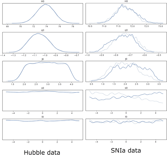
Figure 1. The trace of the free parameters in the cosmographic approach. Left panel: trace of parameters using the Hubble data. Right panel: trace of parameters using SN Ia data.
Download figure:
Standard image High-resolution image3.2. Gaussian Process
The GP approach is a sequence of Gaussian RVs, which can be modeled by considering a multivariate Gaussian distribution. In this case, the diagonal (off-diagonal) terms in the covariance matrix give uncertainty at each point (correlation between different points). Thus, we can model a data set using a GP as

where  is the kernel function and x are the observational points. The μ(x) provides the mean of the RV at each x. Given a set of observations (x, y) and a kernel function, it is straightforward to find (y⋆) at a set of arbitrary points (x⋆). To do this, first of all the mean and covariance matrix of a multivariate Gaussian distribution should be computed from Rasmussen & Williams (2006),

and then the y⋆ can be obtained from sampling of the distribution. In the above equations, CD and Y are the covariance and column vector of data points, respectively.
The most well-known kernel function is the squared exponential, which is given by
In this case,  and σl
are two hyperparameters that must be constrained using a Bayesian inference (Rasmussen & Williams 2006; Seikel et al. 2012). By employing the squared-exponential kernel in the scikit-learn library (Pedregosa et al. 2011), we reconstruct the Hubble parameter (luminosity distance) in the case of the Hubble (SN Ia) data sets.
and σl
are two hyperparameters that must be constrained using a Bayesian inference (Rasmussen & Williams 2006; Seikel et al. 2012). By employing the squared-exponential kernel in the scikit-learn library (Pedregosa et al. 2011), we reconstruct the Hubble parameter (luminosity distance) in the case of the Hubble (SN Ia) data sets.
Having obtained the luminosity distance, it is straightforward to compute the Hubble parameter. The quantity is related to the comoving distance via

and the comoving distance D(z) in a flat geometry is

so in this case we need to take a derivative to obtain the Hubble parameter,

As we mentioned before, we need to take a derivative to compute the cosmographic parameters from the Hubble parameter. In the GP scenarios, it is an easy task to compute not only the first derivative but also other high-order derivatives. In fact, the derivative of a GP is another GP, and one should only compute the mean and covariance matrix of the derivative. All related formulae have been given in Rasmussen & Williams (2006) and Seikel et al. (2012).
Furthermore, we know that the kernel function might influence the results of the GP. Thus, considering the standard Gaussian squared exponential as the main kernel in our analysis, we have used two other Matern-class kernels, Matern (ν = 7/2) (M72) and Matern (ν = 9/2) (M92) (see Mehrabi & Basilakos 2020 for more details on these kernels). The results for both the SN Ia and Hubble data have been presented in Table 1. As is clear from the results, all values are quite in agreement at the 1σ level.
Table 1. Comparison between Different Cosmographic Parameters and Their 1σ Uncertainties, Which Are Obtained Using Different Kernel Functions in the GP Approach
| Hubble Data | SN Ia Data | |||||
|---|---|---|---|---|---|---|
| Kernel | Gaussian Kernel | M72 Kernel | M92 Kernel | Gaussian Kernel | M72 Kernel | M92 Kernel |
| H0∣ | 73.44 ± 1.40 | 73.48 ± 1.36 | 73.45 ± 1.36 | 71.92 ± 0.38 | 71.86 ± 0.40 | 71.99 ± 0.45 |
| q0∣ | −0.856 ± 0.111 | −0.866 ± 0.129 | −0.862 ± 0.118 | −0.558 ± 0.040 | −0.549 ± 0.044 | −0.565 ± 0.056 |
| j0∣ | 1.30 ± 0.37 | 1.29 ± 0.47 | 1.30 ± 0.42 | 0.85 ± 0.12 | 0.819 ± 0.165 | 0.948 ± 0.220 |
Download table as: ASCIITypeset image
3.3. Genetic Algorithm
The latest method that we have used in our analysis is the GA. The early idea of the method comes from Darwin's theory of evolution. According to this scenario, over time and generations, different species evolve and become more compatible with nature. The GA can be regarded as a simulation of the above evolutionary process that is based on an arbitrary set of functions. In this process, a set of trial functions evolves as time passes by through the effect of the stochastic operators of crossover, i.e., the joining of two or more candidate functions to form another one, and mutation, i.e., a random alteration of a candidate function. This process is repeated several times using different random seeds to explore the whole functional space and ensure convergence. Since the GA is constructed as an accidental approach, the probability that a set of functions will bring about offspring is principally assumed to be proportional to a fitness function. We use the χ2 as the fitness function that gives the information on how well every individual agrees with the data.
One of the well-known methods of doing genetic programming is the symbolic regression. Given a set of functions, the symbolic regression generates many mathematical expressions to describe a data set. Each of these expressions has their own χ2 value, which decreases after each generation. Contrary to the GP, the GA is independent of any kernel function, which might affect the results. In this work, we use the public package gplearn, which is an extension of the scikit-learn machine-learning library to perform a symbolic regression. We examine a different set of basic functions and input parameters and find out that a simple (+, −, ×) function set, population size = 2000, tournament size = 30, p crossover = 0.9, p hoist mutation = 0.03, and p point mutation = 0.03 are good inputs to produce reconstructions efficiently.
We run our code several times with different random seeds to generate many reconstructions and then select those with χ2 in the range of  where these quantities can be calculated from the χ2(k) distribution functions. In fact, these upper and lower bands can be calculated by fixing the amount of probability in the χ2(k) distribution. For each data set, we compute k, the number of degrees of freedom, and then from the χ2(k) distribution function,
  have been computed by setting p-value = 0.05. After having a sample of reconstructions, a procedure similar to the GP has been done to compute the mean and standard deviation at each redshift.
4. Results and Discussions
In this section, we report the main results of our analysis using Λ cosmology and different model-independent approaches. The Hubble, deceleration, and jerk parameters have been shown in Figures 2, 3, and 4, respectively. In all plots, the top (bottom) panels) show results considering the Hubble (SN Ia) data. In addition, the 95% (1.96σ) confidence interval for all approaches, as well as the best ΛCDM, has been presented in these plots.
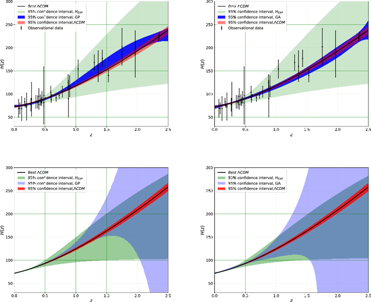
Figure 2. Top panel: 95% confidence interval of the H(z) reconstructions using the Taylor expansion, ΛCDM, GP (left panel), and GA (right panel), as well as observational data points from Hubble data. The wide area indicates the results of the Taylor expansion. Bottom panel: similar to the top panel, but in this case considering the SN Ia data.
Download figure:
Standard image High-resolution image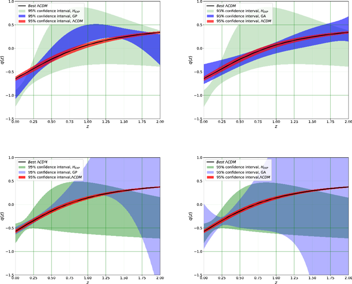
Figure 3. Top panel: 95% confidence interval of the q(z) reconstructions using the Taylor expansion, ΛCDM, GP (left panel), and GA (right panel) from Hubble data. Bottom panel: similar to the top panel, but in this case considering the SN Ia data.
Download figure:
Standard image High-resolution image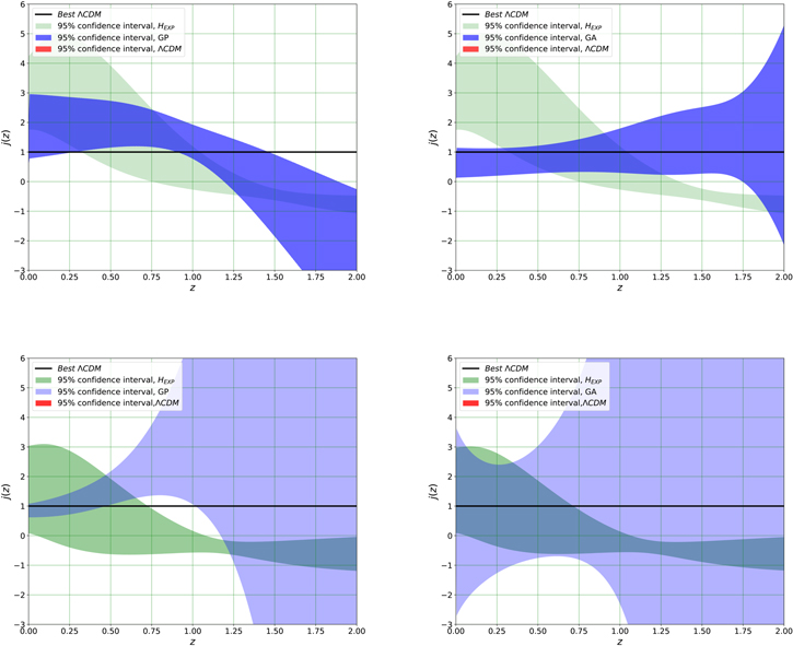
Figure 4. Top panel: 95% confidence interval of the j(z) reconstructions using the Taylor expansion, ΛCDM, GP (left panel), and GA (right panel) from Hubble data. Bottom panel: similar to the top panel, but in this case considering the SN Ia data.
Download figure:
Standard image High-resolution image
Now let us summarize the main aspects of the results for different scenarios:
- 1.Reconstruction of H(z) based on the Hubble data: All reconstructions and their confidence intervals are quite consistent up to redshift z ∼ 0.5. At higher redshifts, the GA is still very well in agreement with the ΛCDM, while the GP results in a small deviation at redshifts (z ∼ 1.5–2). In contrast to these scenarios, the cosmographic approach shows a relatively higher uncertainty at this epoch. This is mainly due to the larger number of free parameters compared to the ΛCDM. The derived value of the H0 in each method has been presented in Table 2.
- 2.Reconstruction of H(z) based on the SN Ia data: The ΛCDM model provides the narrowest region in this case. The results of the GA and the GP are consistent with each other, and there is only a small upper shift in the results of the GP around (z ∼ 1.5–2). The interval region in the cosmographic approach is similar to the Hubble case, but the and the GA give a relatively larger region in particular at z ≥ 1. This is mainly a consequence of the fact that for obtaining the Hubble parameter, we need to take a derivative of the reconstructed function in the GA and the GP. Notice that apart from a large uncertainty at high redshifts, all results are consistent at the 1σ level.
- 3.Reconstruction of q(z) based on the Hubble data: The reconstructions of the deceleration parameters in this case have been shown in the top panel of Figure 3. The result of the GA is quite consistent with the ΛCDM, while the GP's result deviates from the ΛCDM at some redshifts. By the way, these deviations are small, and overall the result is consistent. Similar to the Hubble parameter, the cosmographic approach provides a relatively larger uncertainty compared to the other two methods. Moreover, this method gives a relatively smaller value of the deceleration at the present time. We think that this is probably due to the bias of the model and certainly should be checked in all works that only consider the cosmographic framework for a data analysis.
- 4.Reconstruction of q(z) based on the SN Ia data: The results of all methods are consistent at the present time. Uncertainties in the GP and the GA are quite large at higher redshifts owing to the second derivative that should be computed for obtaining the deceleration. Another important point is that the uncertainty of the GA is much larger than the GP at the present time. This is mainly due to the uncertainty of the numerical derivative at the present time. (The numerical derivative usually fails at the start and end points of a numerical list.) Moreover, the results of the cosmographic approach indicate a biased lower value at redshift ∼2. Similar to the previous one, this is mainly due to the bias of the model.
- 5.Reconstruction of j(z) based on the Hubble data: For the ΛCDM, the value of jerk is constant and is equal to unity. The results of the GA are quite consistent with the ΛCDM, but the GP gives a lower value at higher redshifts. Notice that at these redshifts the uncertainty is large and so the jerk parameter does not deviate significantly. The most important point is the biased value of the jerk at the present time in the cosmographic approach. As is clear in the plots, it provides a value more than 3σ away from the best ΛCDM.
- 6.Reconstruction of j(z) based on the SN Ia data: In this case, all methods give a consistent value with the ΛCDM at the present time. The uncertainties in the GP and the GA are large at high redshifts owing to the effects of taking derivatives. Similar to the deceleration, the uncertainty of the jerk at the present time is much larger in the GA compared to other methods. In fact, a large uncertainty in the deceleration and taking another derivative make the uncertainty at the present time larger compared to the GP.
Table 2. A Summary of the Cosmographic Parameters and Their 1σ Uncertainties, Which Are Obtained Using Different Approaches
| Model∣ | Hexp | GP | GA | ΛCDM |
| Hubble Data | ||||
| H0∣ | 73.88 ± 1.34 | 73.44 ± 1.40 | 71.34 ± 1.74 | 72.08 ± 1.06 |
| q0∣ | −1.070 ± 0.093 | −0.856 ± 0.111 | −0.545 ± 0.107 | −0.645 ± 0.023 |
| j0∣ | 3.00 ± 0.62 | 1.30 ± 0.37 | 0.52 ± 0.24 | 1.00 |
| Pantheon Data | ||||
| Model∣ | Hexp | GP | GA | ΛCDM |
| H0∣ | 71.13 ± 0.46 | 71.92 ± 0.38 | 71.81 ± 1.14 | 71.84 ± 0.22 |
| q0∣ | −0.616 ± 0.105 | −0.558 ± 0.040 | −0.466 ± 0.244 | −0.572 ± 0.018 |
| j0∣ | 1.56 ± 0.74 | 0.85 ± 0.12 | 0.55 ± 1.65 | 1.00 |
Download table as: ASCIITypeset image
Overall, our results indicate that the cosmographic approach is not actually model independent and acts like a model with some free parameters. In the cosmographic method, not only the uncertainties are larger than ΛCDM owing to the larger number of free parameters, but also the method gives some biased values considering the Hubble data. On the other hand, the other two approaches provide much more consistent results. Our results suggest that it might be necessary to consider the GP or the GA (or both) along with the cosmographic approach to confirm the results of the method.
Finally, to present how different approaches perform at the present time, we compute cosmographic parameters at the present time and show the results in Table 2. The top (bottom) section presents results considering the Hubble (SN Ia) data, and 1σ (68%) uncertainty of each quantity has been shown along with the best value. All H0 from the Hubble data are consistent at the 1σ level, and the ΛCDM provides the least uncertainty. For q0, the cosmographic approach provides a smaller value (more than 3σ deviation from the ΛCDM), which is due to the bias of the method. On the other hand, the results of the GA and ΛCDM are quite consistent, but the GP value deviates less than 2σ. For the jerk parameter, we can see a clear (more than 3σ) deviation in value obtained from the cosmography. In this case, the GP provides a consistent value, while the GA gives a value with less than 2σ deviation. Moreover, considering the SN Ia data, all H0 and q0 are consistent with each other at the 1σ level. The values of the jerk parameter are also consistent in this case, but the uncertainty of the the GA is relatively larger than other methods. Our results indicate that for high-quality data like those for SNe Ia, all results are consistent and there is no discrepancy, but for the Hubble data, which are less certain, the cosmographic approach might easily give a biased value.
We have presented the detailed results of different model-independent approaches in Table 3. In this table we report the level of consistency of the results of each method with those of Λ cosmology as a concordance model. Assuming the details of this table, one can easily compare the ability of different model-independent approaches in any epochs of the universe.
Table 3. The Level of Consistency of Reconstructed Cosmographic Functions Using Different Approaches Compared with the Results of Λ Cosmology
| Function | Method | Hubble Data | SN Ia Data | ||||
|---|---|---|---|---|---|---|---|
| Present Value | Low Redshift | High Redshift | Present Value | Low Redshift | High Redshift | ||
| Hexp | 1.7σ tension | consistent | inconsistent | 3.2σ tension | consistent | inconsistent | |
| H(z) | GP | 1.3σ tension | consistent | consistent | 0.4σ tension | consistent | inconsistent |
| GA | 0.7σ tension | consistent | consistent | 0.1σ tension | consistent | inconsistent | |
| Hexp | 18.2σ tension | inconsistent | inconsistent | 2.4σ tension | inconsistent | inconsistent | |
| q(z) | GP | 9.2σ tension | consistent | consistent | 0.8σ tension | consistent | inconsistent |
| GA | 4.3σ tension | consistent | consistent | 5.9σ tension | inconsistent | inconsistent | |
| Hexp | 3.2σ tension | inconsistent | inconsistent | 0.8σ tension | inconsistent | inconsistent | |
| j(z) | GP | 0.8σ tension | inconsistent | inconsistent | 1.3σ tension | consistent | inconsistent |
| GA | 2.0σ tension | consistent | inconsistent | 0.3σ tension | inconsistent | inconsistent | |
Download table as: ASCIITypeset image
5. Conclusion
In the presence of different cosmological models that have been proposed to explain the accelerated expansion of the universe, it will be helpful if one can justify this acceleration without assuming a DE model. Different approaches have been proposed in the literature for this aim, dubbed model-independent approaches. In this paper, we have applied three different kinds of approaches to reconstruct the cosmographic functions from the Hubble data and Pantheon sample. Besides these approaches, we consider the ΛCDM cosmology as a concordance model. The first model-independent approach is built from a Taylor series of the Hubble parameter. Although this approach is widely used in the literature, it suffers from fundamental difficulties with the convergence of the series. To overcome the problem, we have used an improved redshift definition, the y-redshift y = z/(z + 1). For each of the data sets, we perform an MCMC algorithm to find the best-fit value of the free parameters and their uncertainties. In this case, the free parameters are our cosmographic parameters, H0, q0, and j0. Our results indicate that in this analysis we cannot put tight constraints on the other two cosmographic parameters, s0 and l0, and these parameters have no impact on the fitted curve. This result is in full agreement with the results that Rezaei et al. (2020b, 2021) obtained using different data sets.
Furthermore, from the Hubble parameter, we have obtained the evolution of deceleration and jerk functions and their uncertainties as functions of redshift. In this case, not only are the uncertainties larger than those of Λ cosmology owing to more free parameters, but also considering the Hubble data, this method gives some biased values at the present time. In particular, while the value of H0 is relatively consistent with the results of ΛCDM, the values of q0 and j0 are more than 3σ away from that of Λ cosmology (see the results in Table 3). Moreover, using Hubble data, the reconstructed functions obtained from the H expansion method have the larger uncertainties among different methods, especially at higher redshifts.
Assuming SN Ia data, the results are a bit different. In this case the current value of the jerk parameter is consistent with that of the concordance model at about 0.8σ. In this case the Hubble function reconstructed using the H expansion method is consistent with ΛCDM at redshift range z < 1, while in higher redshifts and for the other cosmographic functions the results are disappointing.
The second model-independent approach we have used in this paper is the GP. The H(z) and q(z) functions that have been reconstructed from Hubble data using this approach are consistent with the concordance model, especially at lower redshifts. Assuming SN Ia data at higher redshift, the results of the GP decouple from those of Λ cosmology. In the case of the jerk function, the results of the GP are not acceptable, except for low-redshift SN Ia data points.
The last model-independent approach we have used in this work is the GA. By the GA and using Hubble data, we reconstruct H(z) and q(z) functions, completely close to the results of ΛCDM. These results repeated when we use Hubble data to reconstruct the jerk function, but just at low redshifts. Assuming SN Ia data in this approach leads to good reconstruction of H(z) at z < 1, while in the other cases, the GA with SN Ia data failed in reconstruction of cosmographic functions.
At the present time, for the Hubble data and the SN Ia data, the predicted H0 value using the GA is consistent with the ΛCDM at the < 0.7σ level. Moreover, considering the Hubble data, all of the approaches give a value of q0 completely away from the q0 of ΛCDM, except GA, which provides less deviation from the results of ΛCDM. For the jerk parameter (j0), results of the GP using both data samples are consistent with the ΛCDM model at about the 1σ confidence level. On the other hand, H expansion and the GA lead to good results for j0, just by considering the SN Ia data.
In addition, at intermediate redshifts (z ∼ 0.5–1.3), performance of the GP and the GA is comparable with ΛCDM, while the cosmographic approach provides a larger uncertainty. In contrast, for SN Ia data at higher redshifts, the uncertainties in q(z) and j(z) from the GP and the GA are relatively larger than those of H expansion methods. This is mainly due to taking the derivative of the reconstructed function. Summarizing all of the above results, we can say that for reconstruction of H(z), the GA is the more consistent method, followed by GP. In reconstructing the deceleration function, none of the approaches lead to consistent results, but among them the GP was better than the others. In order to reconstruct j(z), the GA and the GP lead to relatively good results, while the results of the H expansion approach are disappointing. Overall, we conclude from these results that the cosmographic approach cannot reconstruct cosmographic functions exactly, especially at higher redshifts. This method performs like a model with more free parameters, and this makes errors larger than those of the ΛCDM. In addition, comparing to the other methods applied in this work, this method is not flexible enough to fit the data better than the ΛCDM. For both data samples, the other two model-independent methods provide more consistent results compared to the concordance model. It is confirmed that the cosmographic approach gives biased results. Therefore, we suggest that for confirming any tension in analyzing a data set, especially at high redshifts, it might be necessary to consider a more sophisticated model-independent method like the GP and the GA besides using the cosmographic approach.