


Abstract
A joint X-ray (0.2–2 keV) and ultraviolet (1150–3000 Å) time-domain study has been carried out on three nearby bright late-type stars, bracketing the Sun in properties. Alpha Cen A (HD 128620: G2 V) is a near twin to the Sun, although slightly more massive and luminous, slightly metal-rich, but older. Alpha Cen B (HD 128621: K1 V) is cooler than the Sun, somewhat less massive and lower in luminosity. Procyon (HD 61421: F5 IV–V) is hotter, more massive and more luminous than the Sun, half the age, but more evolved. Stellar observations were from Chandra X-ray Observatory and Hubble Space Telescope (HST). The Sun provided a benchmark through high-energy spectral scans from solar irradiance satellites and novel high-dispersion full-disk profiles of key UV species—Mg ii, C ii, and Si iv—from the Interface Region Imaging Spectrograph. Procyon's flux history was strikingly constant at all wavelengths, in contrast to the other three cycling-dynamo stars. Procyon also displays a strong subcoronal (T ∼ 1 × 10⁵ K) emission excess, relative to chromospheric Mg ii (T ≲ 104 K), although its X-rays (T ∼ 2 MK) appear to be more normal. At the same time, the odd sub-Gaussian shapes, and redshifts, of the subgiant's "hot lines" (such as Si iv and C iv) are remarkably similar to the solar counterparts (and α Cen AB). This suggests a Sun-like origin, namely a supergranulation network supplied by magnetic flux from a noncycling "local dynamo."
Export citation and abstract BibTeX RIS
1. Introduction
This is the fifth in a series that is intended to more firmly establish the Sun's place among the stars, especially the denizens of the solar neighborhood, whose proximity and brightness allow detailed examinations from the ground and space, to a degree unmatched by more distant objects. "Trenches" mainly focuses on soft X-ray (0.2–2 keV; 6.2–62 Å) and ultraviolet (1150–3000 Å) emissions of Sun-like stars (i.e., those near 1 M⊙). The high-energy emissions are manifestations of the magnetic activity that is broadly found in the cool half of the Hertzsprung–Russell (H–R) diagram. Stellar magnetism is attributed to at least two classes of magnetohydrodynamical phenomena. The most familiar is an internal dynamo (Parker 1970) that derives its power from rotation and convection. Less commonly appreciated is a surface (or local) dynamo (Nordlund et al. 1992) that is thought to be purely convection-driven. The internal dynamo is responsible for the long-term activity cycling of the Sun, which is most conspicuous as the iconic 11 yr ebb and flow of sunspots. Analogous activity modulations were recognized in the stars through a decades-long survey of chromospheric proxy Ca ii H & K (∼3950 Å) at Mount Wilson Observatory (Wilson 1978). The internal dynamo is also conflated with the strong evolution of activity. Young, fast-spinning stars—hyperactive by measure of X-ray and UV luminosities—quickly fade in high-energy emissions over just a few hundred million years as the stellar rotation is relentlessly braked by the magnetized coronal wind. Meanwhile, the local dynamo is thought to operate independently of stellar rotation, and should mainly respond to fundamental stellar properties, such as surface temperature and gravity, which change only slowly over evolutionary timescales.
The focus on high-energy emissions stems partly from a desire to understand the underlying energy release mechanisms, which can inspire extremely hot, nonclassical temperatures (105–107 K) in the outer atmospheres of otherwise cool stars (Teff ∼ 3000–6500 K), and violent transient energy bursts known as flares. The "space weather" (SW) associated with the Sun's high-energy activity is additional motivation, especially flares and mass ejections. These energetic events can storm through the heliosphere and potentially harm vulnerable infrastructure on, or around, Planet Earth. Furthermore, the oftentimes more severe versions of SW on other stars (especially the red dwarfs) can wreck havoc on the surfaces and atmospheres of their inner exoplanets, which creates additional hurdles for habitability (e.g., Airapetian et al. 2020).
Paper I (Ayres 2020) followed solar soft X-ray and UV irradiances (Sun as a star) over a 17 yr period (2003–2020) covering the decline of sunspot Cycle 23, and the rise and fall of subsequent Cycle 24 (albeit a modest one as cycles go). The (daily) solar fluxes were contrasted with semiannual X-ray and UV time series of the two Sun-like stars of the nearby α Centauri triple system ("A" (HD 128620): G2 V; "B" (HD 128621): K1 V; d = 1.34 pc), which have been collected for more than a decade jointly by the Chandra X-ray Observatory and Hubble Space Telescope (HST). Near-solar-twin α Cen A closely paralleled the behavior of the Sun in the various important UV emission lines and broadband X-rays, which is perhaps not surprising considering that the two early-G stars are so similar, but encouraging nonetheless to counter any ideas that the Sun might somehow be exceptional. At the same time, several of the pivotal solar/α Cen A trends were curiously at odds with previous stellar experience, guided by earlier studies of generally more active stars (the α Cen K-type secondary adhered to the previous lore more closely; K dwarfs tend to be more active than G-types at the same age).
Paper II (Ayres 2021a) switched gears to the Sun's extreme ultraviolet (EUV: 100–1150 Å), as recorded over 2010.5–2020, during the maximum and decline of Cycle 24. EUV radiation is also significant for solar and exoplanetary SW reasons, but the key wavelengths between 350 and 912 Å are strongly absorbed by the interstellar medium, and are essentially unobservable, even in the nearest stars. Nevertheless, correlations of bright EUV emissions (e.g., He ii 303 Å: 8 × 10⁴ K) versus counterparts in the FUV (e.g., Si iv 1393 Å: 8 × 10⁴ K) can be used to construct proxy models of the EUV spectrum for stars, at least those not too different from the Sun. These "flux–flux" correlations also are of interest to atmospheric modelers simulating the complex energization and cooling of the hot corona and associated transition layers.
Paper III (Ayres 2021b) broadened the stellar context for "Trenches" by describing a sample of nearly 50 early-F to early-K Sun-like dwarfs, observed in the 1150–1420 Å short end of the far-ultraviolet (FUV: 1150–1700 Å) using the extremely sensitive Cosmic Origins Spectrograph (COS) on HST. Targets were chosen from the North and South Ecliptic polar regions because these locations receive much deeper exposures by contemporary scanning satellites, such as TESS and eROSITA, which can provide vital ancillary information—optical and X-ray variability, respectively—that is not easily obtained otherwise. The minimally biased "Ecliptic-poles Stellar Survey" (EclipSS) was dominated by stars of low activity similar to the Sun, as gauged by midchromosphere O i 1306 Å and upper-chromosphere C ii 1335 Å. A hard lower ("basal") boundary on the chromospheric emissions reinforced the idea (e.g., Judge & Saar 2007) that a minimum, baseline level of activity is powered by the supergranulation network, essentially independently of the stellar rotation rate. (The Sun's network is a widespread pattern of small scale patches of magnetic flux, which is mainly populated by the local dynamo and organized by large-scale horizontal convective flows.) The implication is that significant UV (and likely also X-ray) emissions would be present even when starspots and associated active regions were absent from the stellar surface (e.g., the Sun for nearly seven decades during the 17th century "Maunder Minimum", Eddy 1976).
Paper IV (Ayres et al. 2021) returned to the Sun to pave the way for subsequent comparisons of high-spectral-resolution solar and stellar UV spectra (as here in current Paper V). Paper IV analyzed a unique set of full-disk raster scans of the Sun, covering important bright chromospheric (T ≲ 104 K) and transition zone (TZ: ∼ 105 K) lines, collected by the Interface Region Imaging Spectrograph (IRIS), which is a NASA Small-Explorer satellite. Full-disk ("Sun as a star") line profiles were assembled from the mosaics of key species: Mg ii, C ii, and Si iv. The disk-average solar profiles can directly be compared to stellar counterparts, such as from the HST/STIS echelles, at comparable resolution. The full-disk line shapes, solar or stellar, are formed by taking an average over many different types of emitting structures, with their own internal thermal and kinematic characteristics, and whose radiation is altered to varying degrees by center-to-limb intensity effects. Consequently, the full-disk profiles are shaped by vastly more influences than, say, a single high-spatial-resolution spectrum from some arbitrary point on the disk. Of course, that global-scale information is hopelessly jumbled together and is heavily encrypted. Nevertheless, in contrast to the stellar examples, the IRIS mosaics pervasively sampled the disk at high-spatial resolution, so it was possible to link specific regions on the surface with specific aspects of the full-Sun profiles. In that way, pivotal contributions to the full-disk averages could be recognized, such as a bright-limb ring for Si iv, and a progressive domination by the supergranulation going from cooler Mg ii to warmer C ii to hotter Si iv. The latter is almost exclusively associated with the network at the low points of the sunspot cycle (all of the diagnostics had substantial contributions from active regions during the high points).
An intriguing aspect of this study was the recognition that the non-Gaussian line shape of optically thin TZ Si iv, which was previously addressed in the solar and stellar contexts by a bimodal combination of narrow and broad Gaussians, could successfully be modeled by a pseudo-Gaussian profile, in which the normal Gaussian exponent a = 2 was allowed to take on other values. The more peaked Si iv profile typically had a < 2, whereas the boxier optically thick chromospheric lines C ii and Mg ii typically had a > 2. Significantly, the sub-Gaussian line shapes of Si iv seen in the full-disk average could be followed down to the finest spatial scales of the IRIS mosaics. This suggested that whatever mechanism was responsible for the non-Gaussian line profiles, kinematic or not, was intrinsic to the smallest spatial scales and was not simply a combination of one profile shape in one region and a second, different shape from another location (which is otherwise a viable option for an unresolved stellar spectrum).
The most profound finding of Paper IV, in terms of the solar-stellar connection, was that the spatially resolved emission-line strengths from quiet areas on the Sun to extreme active regions mirrors the full span of variation (≳10), from disk-average quiet stars such as the Sun all the way to much more active 50 Myr old cousins, such as EK Draconis (e.g., Ayres 2015a). This was in spite of the rather modest full-disk intensity contrasts in most of the UV lines displayed over Cycle 24 from MIN to MAX (less than a factor of 2). The implication was that the physical processes that cause widespread heating on the surfaces of hyperactive stars have analogs in the most intense cores of active regions on the observationally much more accessible Sun.
In the current Paper V, the insights gained in the study of the IRIS solar full-disk mosaics were applied to the existing STIS high-spectral-resolution profiles of α Cen A and B (hereafter AB), already described in earlier papers of this series but treated previously according to integrated fluxes rather than resolved line shapes. Furthermore, a new stellar protagonist was introduced: the mid-F subgiant Procyon (α Canis Minoris A (HD 61421): F5 IV–V).
Procyon has been followed for over a decade by Chandra and HST/STIS, initially in unconnected programs, but more recently in a dedicated joint effort. Procyon is a significantly different type of star than α Cen AB or the Sun: it is hotter, more luminous, and more massive; it is younger, but more advanced from an evolutionary perspective. Nevertheless, Procyon is technically still a Sun-like star, and is one of the closest of the ∼1 M⊙ objects to Earth (d ∼ 3.5 pc versus 1.3 pc for α Cen).
As a nearby bright star, Procyon was an early subject of chromospheric modeling, together with α Cen AB (Ayres et al. 1974, 1976). These studies, and others, demonstrated that chromospheric temperature distributions of all three stars qualitatively agreed with the best available solar models of the day. Later, it was recognized by Simon & Drake (1989) that F stars such as Procyon tended to display sub-luminous coronal soft X-rays compared with FUV species, such as C iv. These anomalous stars were called "X-ray deficient," and in the case of Procyon the deficit was about 1 dex. Simon & Drake suggested that the coronal dichotomy, with a break at around F5, might be associated with a transition from acoustic-type heating—a popular alternative at the time (e.g., Stepien & Ulmschneider 1989)—in the earlier Fs, to a magnetic dynamo process among the later Fs. However, Ayres (1991) countered, in the specific example of Procyon, that the narrow widths and apparent redshifts of high-temperature lines such as C iv 1548 Å recorded in International Ultraviolet Explorer (IUE) echelle spectra were similar to those seen among the later types. Narrow lines were incompatible with high fluxes of sound waves passing through the TZ, and the redshifts were taken to indicate downdrafts of hot material (∼105 K) at the footpoints of coronal magnetic loops, as seen on the Sun. Alternatively, the lack of rotational modulations in Procyon's FUV in the Ayres (1991) study might be viewed as supporting the absence of spatially concentrated active regions, which are a hallmark of dynamo activity among the later types. Notably, the traditional acoustic wave heating should be spatially uniform.
The Ayres (1991) "Many Faces of F Stars" concluded: "Thus the present work should be viewed as a progress report concerning an issue whose resolution lies in the future. Indeed, the global problem of chromospheric heating across the H–R diagram in many ways is like that which confronts solar physicists: no single simple theory can readily explain the sometimes subtle, sometimes vivid structure that is seen. Perhaps as our view of the stars becomes more "solar-like," with the advent of HST, we will uncover a profound connection between the curious boundaries in spectral type and luminosity where the manifestations of chromospheric heating undergo fundamental transformations and the dazzling array of fine structure that so ubiquitously mottles the Suns surface." It could be said that the future envisioned 30 years ago has now arrived.
This paper is structured as follows. The first section describes the properties of the three subject stars, focusing on the new addition, Procyon. The second section outlines the existing Chandra observations, mainly of Procyon but also noting a recent pointing on α Cen obtained subsequently to Paper I, and including discussion of a revised solar X-ray time series, which has recently supplanted the version used in Paper I. Next, the HST/STIS visits on all three stars are summarized, including more detailed supporting information than was needed for the simple integrated fluxes of Papers I and III. An analysis section describes the emission-line fitting methodology, and presents summaries of various correlations among the profile shape parameters of the stars; as well as "flux–flux" diagrams comparing pair-wise strengths of various emission lines, or coronal X-rays, including the trends previously obtained for the Sun (flux–flux correlations were a staple of the earlier "Trenches" episodes). The final section includes the discussion and conclusions. In addition, Appendix A describes modifications to the curved power-law relations presented in Papers I and II for solar UV and EUV lines against coronal X-rays, based on the recently revised solar X-ray time series. Appendix B outlines corrections to the STIS echelle wavelength scales derived from a new analysis of wavelength calibration material. Finally, Appendix C illustrates additional spectral fits to both medium- and high-resolution epoch-average STIS UV spectra of α Cen B and Procyon, beyond the medium-resolution example of α Cen A described in the main body of this article.
2. Observations
2.1. The Stellar Players
Table 1 summarizes the fundamental properties of the three STIS stars. The values for α Cen AB were copied from Paper I, and are mainly drawn from Kervella et al. (2017). The two dwarfs closely bracket the Sun in mass, radius, and luminosity. Alpha Cen A is similar in temperature to the Sun, while B is several hundred K cooler, befitting its later spectral type. The α Cen system is slightly metal-rich compared to the Sun, by about 0.2 dex. Even though, in principle, a binary system with accurately known masses, luminosities, and composition should tightly constrain the age through evolutionary considerations, estimates for AB span a broad range. Consensus values suggest that the system is roughly 1 Gyr older than the Sun.
Table 1. Stellar Properties
| Name | HD No. | Type | M/M⊙ | R/R⊙ | LBOL/L⊙ | Teff | [Fe/H] | fBOL | υROT |
|---|---|---|---|---|---|---|---|---|---|
| (K) | (erg cm−2 s−1) | (km s−1) | |||||||
| α Cen A | 128620 | G2 V | 1.11 | 1.22 | 1.52 | 5800 ± 20 | +0.24 | 2.718 × 10⁻⁵ | 2.1–2.8 |
| α Cen B | 128621 | K1 V | 0.94 | 0.86 | 0.50 | 5230 ± 20 | +0.24 | 0.899 × 10⁻⁵ | 1.1 |
| Procyon (α CMi A) | 61421 | F5 IV–V (+DZQ) | 1.48 | 2.03 | 6.89 | 6560 ± 90 | +0.00 | 1.79(±0.09) × 10−5 | 6 |
Note. Parameters for α Cen AB from Paper I. See text for discussion of Procyon values.
Download table as: ASCIITypeset image
Procyon is the nearest of the F-type stars and is one of brightest. Technically, it is solar-like, with M ∼ 1.5 M⊙ and a temperature only 800 K warmer than the Sun's. However, unlike the Sun, Procyon is a subgiant, on a post-main-sequence track heading toward the red giants. Like AB, Procyon is in a visual binary, although the companion is a faint, hydrogen-deficient, metal-polluted white dwarf, which indicates that the system has witnessed significant evolution over its lifetime and that the current primary was once the secondary. Procyon's apparent orbit on the sky is compact (semimajor axis ∼4 3) and the period is a relatively short 41 yr. Orbital elements were challenging to determine historically, given the difficulty to recover the very faint secondary in the glare of the close-by bright primary. In the spacecraft era, Bond et al. (2015) used high-precision HST imaging to track about half the orbital path and, combined with the historical astrometry, significantly refined the parameters. The inclination of the system is low, about 31°, and the eccentricity is high, e ∼ 0.40. The inferred mass of Procyon is 1.48 ± 0.01 M⊙.
As of 2021 June, SIMBAD listed nearly a hundred Teff entries for the subgiant, although some are duplicates. A consensus 6560 ± 90 K encompasses the recently proposed values. Most of the metallicities cited in SIMBAD are indistinguishable from solar, and much of the evolutionary modeling cited below has assumed solar composition (although, to be sure, there still are heated debates as to what constitutes the true solar scale, as noted below).
A detailed study by Aufdenberg et al. (2005) had superseded an earlier effort by Kervella et al. (2004), who measured the interferometric radius of Procyon with the VLT. Aufdenberg et al. derived fundamental parameters for the subgiant utilizing 3D convection models to establish the critical limb-darkening factors needed to interpret the interferometric measurements. The derived radius is 2.03 ± 0.01 R⊙, and the effective temperature estimate is 6540 ± 80 K.
Age is a key factor in coronal activity, but is challenging to determine for arbitrary Field stars. As mentioned earlier, binary systems with known masses and compositions offer additional constraints on the stellar age through the joint evolution. Nevertheless, these efforts have led to a disappointingly wide range of estimates for Procyon, partly because the current secondary has essentially finished its life and thus offers less of a lever arm than would a currently evolving Main sequence companion. Bond et al. (2015) cite ages of 1.7–2.7 Gyr, which they obtained with different assumptions concerning core convective overshooting, and note that the asteroseismic age is on the higher side. An earlier evolutionary study by Liebert et al. (2013) proposed a tighter range, 1.9 ± 0.1 Gyr, using the Asplund et al. (2005) solar abundance scale (Z = 0.015); and a slightly higher value, 2.0 Gyr, with the Grevesse & Sauval (1998) composition (Z = 0.019), although the authors reported that the latter model fits were poorer. According to these authors, part of the difficulty in pinning down the age of mid-F stars such as Procyon is the importance of overshooting, given the small convective cores and thin convective envelopes. More recently, Sahlholdt et al. (2019), in a study of Gaia Benchmark stars (Procyon is one), proposed 1.5–2.5 Gyr for the F subgaint, with 2 Gyr the preferred age, again based on model tracks and seismology. It seems likely that Procyon is substantially younger than the Sun or α Cen, by perhaps 2–3 Gyr, yet is more advanced in its evolution. Thus, it is a unique comparison star as far as the state of its magnetic activity is concerned, especially in terms of its core and envelope structure at the edge of convection.
Another key dynamo parameter is the rotation rate. An attempt was made by Ayres (1991), alluded to earlier, to record rotational modulations of bright FUV lines of Procyon, including H i 1215 Å Lyα, using high-S/N trailed exposures with the low-dispersion SWP mode of IUE, but without success. Allende Prieto et al. (2002) reported  km s−1 based on high-quality optical absorption spectra of Procyon from the McDonald Observatory (∼1.5 km s−1 resolution; S/N up to 2000), which was interpreted with the help of 3D radiation-hydrodynamic convection models. The authors cautioned that the projected velocity might be overestimated by as much as 0.5 km s−1 owing to subtleties associated with the finite numerical resolution of the simulations. Earlier, Gray (1981) had obtained 2.8 ± 0.3 km s−1 for Procyon, also using high-resolution McDonald spectra, but with a novel Fourier analysis that was popular at the time. Taking a compromise
  km s−1, and assuming that the spin axis of the star is aligned with the orbit, implies a rotational velocity of 6 km s−1 and a period of about 17 days, which is somewhat shorter than the midlatitude solar value of 25 days.
The last important parameter is the bolometric flux, fBOL (erg cm−2 s−1 at Earth), which will later be used to normalize the UV fluxes to allow a fairer comparison among the three stars of the study, which differ significantly in sizes and distances. The usual approach for arbitrary late-type stars is to apply a formula based on, say, the Gaia broadband G magnitude and the Gaia (bp − rp) color (see, e.g., Paper III, Appendix A). Alternatively, nearby bright stars such as Procyon often have detailed spectral irradiance coverage, extending from the FUV up into the mid-infrared. The broad spectral energy distributions can be integrated directly to yield a higher quality estimate of fBOL than could be obtained from, say, the G-based formula, especially given that nearby stars such as Procyon (and α Cen AB) are too bright for Gaia, so G magnitudes and colors are lacking in the first place. Aufdenberg et al. (2005) carried out such a SED integration for Procyon, and found fBOL ∼ 1.79 ±0.09 × 10⁻⁵ erg cm−2 s−1, which is adopted here.
2.2. Chandra X-Ray Observatory
The High-Resolution Camera (HRC-I) of the Chandra X-ray Observatory has been especially valuable in the study of nearby optically bright late-type stars that also have high count rates in the 0.2–2 keV soft X-ray band. HRC-I is immune to "optical loading," the impact of low-energy photons on CCD-type X-ray detectors, which requires either blocking filters or short frame times to mitigate; as well as "pile-up," the collision of multiple X-ray photons in a single cell of a CCD detector during the integration time. HRC-I also retains excellent sensitivity to the softer X-ray emission typical of low-activity coronae such as the Sun's, whereas the CCD cameras of Chandra have lost significant low-energy response owing to layers of molecular contamination that have built up over the years. The one downside of HRC-I is its lack of energy resolution compared to CCD cameras, which typically achieve modest but useful E/ΔE ∼ 50. However, the poor spectral response of HRC-I is countered by its relatively constant energy conversion factor (ECF: erg cm−2 counts−1) over the 1–10 MK coronal temperature range favored by nearby low- and moderate-activity stars. Furthermore, several of the nearby bright stars have been subjected to detailed high-resolution X-ray spectroscopy with Chandra's Low-Energy Transmission Grating Spectrometer (LETGS: E/ΔE ∼ 500–1000). Models of the distribution of coronal plasma with temperature, and associated coronal abundances, can be derived from these high-quality X-ray spectra (e.g., Wood et al. 2018, and references to previous work therein); in fortuitous cases, at extremes of activity cycles (Ayres 2015b for AB; LETGS pointings on Procyon were also included in that study).
Long-term X-ray imaging programs have been carried out on α Cen AB with HRC-I since late-2005. The subarcsecond spatial resolution of Chandra has been vital given that the AB orbital separation was shrinking over that period, bottoming out at 4'' in 2016, and will continue to be below 10'' (approximate resolution of XMM-Newton) until the latter part of the current decade. Since 2010, the Chandra program has been conducted jointly with HST/STIS, which will be covered in more detail later. The long-term Chandra HRC-I program on α Cen AB was described in Paper I. Table 2 provides an additional Chandra pointing carried out recently, after publication of Paper I.
Table 2. Chandra HRC-I Pointings: α Cen AB (New: post-2020.1)
| ObsID | UTmid |

| (CR)A | (CR)B |

|

|
|---|---|---|---|---|---|---|
| (yr) | (ks) | (counts s−1) | (1027 erg s−1) | |||
| 1 | 2 | 3 | 4 | 5 | 6 | 7 |
| 21575 | 2020.428 | 5.11 | 0.49 ± 0.06 | 3.90 ± 0.44 | 0.29 | 3.87 |
Note. Col. 3 exposure time includes dead-time correction. Cols. 4 (A) and 5 (B) count rates were time-filtered to remove flare enhancements, if any; and were corrected for the 95% encircled energy of the r = 15 detect cell. Cited uncertainties reflect standard deviations of time-binned count rates, including the influence of flares, with respect to reported flare-filtered averages. Cols. 6 (A) and 7 (B) X-ray luminosities (0.2–2 keV) were calculated from the count rates using CR-dependent ECFs derived for A and B separately (see Ayres 2014 for further details), and d = 1.338 pc (e.g., Kervella et al. 2017). No correction was made for the time-dependent sensitivity decline of HRC-I (about 2% per year since 2010).  in same energy band and luminosity units, over recent (weak) sunspot Cycle 24.
Download table as: ASCIITypeset image
Procyon has been observed by Chandra sporadically since early in the mission, mainly with LETGS (+HRC-S camera) prior to 2016, although with one High-Energy Transmission Grating Spectrometer (HETGS+ACIS-S) pointing (2014) and a single on-star HRC-I exposure (2008). In 2016, a dedicated joint Chandra/HST project (HRC-I + STIS) was approved, which has continued to the present. Initially, the program featured semiannual 10 ks exposures of the subgiant, which were scaled back to 5 ks integrations roughly annually in recent years (for reasons that will become obvious shortly). Procyon is a bright, ∼1 count s−1 X-ray source, which can yield a high-S/N detection in 1 ks. However, the longer duration exposures guarded against short-term flare events, which had previously been seen in α Cen B pointings, and can skew the measurement away from the desired quiescent level in that epoch (Ayres 2014). However, no such flaring was detected in any of the Procyon light curves.
Table 3 lists all of the HRC-I pointings on Procyon through 2021 April. On the one hand, the zeroth-order images of the LETGS (or HETGS) spectra could have been measured to provide additional points on the X-ray time history of Procyon (and those of AB as well). On the other hand, the HRC-I exposures alone are sufficient for the purpose, and avoid the uncertain scaling between the attenuated zeroth-order image and a direct HRC-I exposure.
Table 3. Chandra HRC-I Pointings: Procyon (post-2008.0)
| ObsID | UTmid | texp | CR | LX |
|---|---|---|---|---|
| (yr) | (ks) | (counts s−1) | (1027 erg s−1) | |
| 1 | 2 | 3 | 4 | 5 |
| 8908 | 2008.020 | 4.78 | 1.54 ± 0.02 | 8.7 |
| 18304 | 2016.183 | 9.68 | 1.37 ± 0.01 | 7.6 |
| 18305 | 2016.685 | 10.06 | 1.43 ± 0.01 | 8.0 |
| 18306 | 2017.254 | 10.03 | 1.39 ± 0.01 | 7.7 |
| 18307 | 2017.713 | 9.95 | 1.33 ± 0.01 | 7.4 |
| 18308 | 2018.128 | 9.99 | 1.32 ± 0.01 | 7.3 |
| 18309 | 2018.692 | 9.76 | 1.31 ± 0.01 | 7.2 |
| 21578 | 2019.406 | 5.01 | 1.23 ± 0.02 | 6.7 |
| 21579 | 2020.051 | 5.07 | 1.23 ± 0.02 | 6.7 |
| 21580 | 2021.261 | 5.09 | 1.24 ± 0.02 | 6.8 |
Note. Col. 3 exposure times include dead-time corrections. Col. 4 count rates were corrected for the 95% encircled energy of the r = 15 detect cell. Cited uncertainties reflect Poisson noise. Col. 5 X-ray luminosities (0.2–2 keV) were calculated from the count rates using a CR-dependent ECF (see Ayres 2014 for details), and d = 3.514 pc (from the Hipparcos ϖ: van Leeuwen 2007). No correction was made for the time-dependent sensitivity decline of HRC-I.
Download table as: ASCIITypeset image
The Chandra HRC-I event lists were processed as described in Ayres (2014), incorporating count-rate-dependent ECFs developed specifically for α Cen AB and Procyon based on emission-measure modeling of the respective LETGS spectra. Fortuitously, the three available epochs of LETGS spectra of AB, taken over about 11 yr, happened to capture coronal low and high states of both stars, so the hardening of each SED toward the cycle MAX could be tracked. One further note: the HRC-I has declined in sensitivity for soft coronal sources by about 20%–30% since 2010, according to WebPIMMS. 1 The sensitivity decline was not compensated for the X-ray luminosities in Tables 2, but was taken into account in subsequent figures involving the coronal emissions (as described below).
2.2.1. Solar X-Rays: Revised FISM2
The solar X-ray time series utilized in Papers I and II was a then recently updated version of the so-called Flare Irradiance Spectral Model (FISM), which is available from the LISIRD 2 irradiance interface hosted by the Laboratory for Atmospheric and Space Physics at the University of Colorado. FISM incorporates a variety of inputs, including direct measurements of broadband solar X-rays by means of filtered diode sensors, as well as proxy relations, and folds the inputs though an emission-measure model to calculate a moderate-resolution high-energy spectrum between 0.1 Å and 1900 Å. The new version at the time, called FISM2, increased the wavelength sampling and resolution of the spectral modeling, among other enhancements. The main difference between FISM2 and original FISM in the 0.2–2 keV soft X-rays was that the cycle minima of FISM2 were at higher intensities than those of FISM (see Figure 8 of Paper I). The FISM2 X-ray time series 2003–2020 (Paper I) and 2010–2020 (Paper II) were utilized for a variety of purposes, mainly to construct "flux–flux" diagrams by pitting the coronal X-rays against other atmospheric tracers, such as chromospheric Mg ii and subcoronal C iv. Typically, flux−flux diagrams that compare hot X-rays against a cooler diagnostic such as Mg ii follow power laws with indices α ≳ 3, which indicates that the X-ray activity increases rapidly with increasing chromospheric intensity.
More recently, in 2021 March, a new version of FISM2 was released, again with numerous improvements. Curiously, the new version sports deeper cycle minima than the previous FISM2, returning the peak/minimum cycle contrast to about 10 from the previous factor of 5. Appendix A illustrates the revised FISM2 long-term X-ray history of the Sun, and new power laws with respect to EUV and UV species, to replace the ones derived in Papers I and II based on the earlier version of FISM2.
2.2.2. X-Ray Time Histories of the Sun-like Stars
Figure 1 depicts time histories of bolometrically normalized coronal emissions of the Sun, α Cen AB, and Procyon, from about 2005 to the present. The Chandra points were corrected for a somewhat arbitrary 2% per year HRC-I sensitivity decline since 2010. This particular slope was chosen because it flattens the recent Procyon HRC-I time series, which would be consistent with the stable long-term behavior shown by the earlier LETGS spectra (and the one HRC-I from 2008). The lower panel highlights epochs when HST/STIS pointings on the three stars were carried out. An upward pointing triangle indicates that an FUV spectrum was obtained; a diamond indicates FUV + NUV.

Figure 1. Soft X-ray time histories of α Cen A (blue dots), α Cen B (red), Procyon (green), and the Sun (gray points are daily values; larger dark dots are 81 day (3-rotation) averages). The lower panel highlights epochs when HST/STIS pointings were carried out (same color-coding as in main panel).
Download figure:
Standard image High-resolution imageThe Sun displays one complete 11 yr cycle (Cycle 24) and the tail of preceding Cycle 23. Alpha Cen B shows one 8 yr cycle, and much of a second currently in progress. Alpha Cen A has most of a 19 yr cycle in the Chandra epochs, including a long minimum between 2005 and 2010; α Cen A had an earlier peak in the late 1990s bridging the end of the ROSAT mission and beginning of Chandra's (see Ayres 2014). The Procyon time series is flat, somewhat by design given the assumed sensitivity decline of HRC-I. However, if the true decline is less, or more, then it would only tilt the Procyon time series up or down by a small amount, preserving the long-term trend of relative constancy, certainly when compared to the rather larger excursions exhibited by the other stars. It is possible, in fact, that Procyon fortuitously is an excellent calibration star to document HRC-I's soft response over time.
2.3. Space Telescope Imaging Spectrograph
The medium-resolution (λ/Δλ ∼ 45,000) and high-resolution (λ/Δλ ∼ 110,000) UV echelle modes of STIS are well-suited for nearby bright late-type stars, in terms of sensitivity, photometric stability, and wavelength precision (as validated by frequent calibration exposures of onboard hollow-cathode lamps). The long-term UV campaigns on α Cen AB were described in Paper I and also by Ayres (2015b). A newer set of observations of AB occurred in early-2021, after publication of Paper I. The STIS material for Procyon comes from two efforts. The first was the Advanced Spectral Library Project (ASTRAL 3 ), which obtained full UV coverage of Procyon—in medium- and high-resolution in the FUV, and high-resolution in the NUV—over seven separate HST visits between 2011 April and October. The second effort was a recent joint Chandra/HST campaign, which has been collecting more focused FUV and NUV spectra (the latter capturing the important Mg ii doublet at 2800 Å) since 2016, initially semiannually but more recently annually.
Table 4 is a catalog of the STIS echelle observations utilized here, of the three reference stars. A few blank exposures are excluded from the inventory owing to various types of failures, especially associated with Guide-Star reacquisitions. Usually, the failed observations were repeated within a few months. All of the FUV pointings on Procyon are included but only the NUV exposures that captured the Mg ii hk doublet, the main spectral target of interest here at the longer wavelengths. The table contains additional information, beyond the exposure specifications and epochs, namely empirical radial velocities and NUV flux scale factors.
Table 4. HST/ STIS Pointings: α Cen AB and Procyon
| ObsNUM | ObsID | UTmid | Setting | Aperture | Range |

| S/N | RVF | RVN |

|
|---|---|---|---|---|---|---|---|---|---|---|
| (yr) | ('')×('') | (Å) | (s) | (km s−1) | ||||||
| 1 | 2 | 3 | 4 | 5 | 6 | 7 | 8 | 9 | 10 | 11 |
| α Centauri A | ||||||||||
| 1A | ob8w01010 | 2010.065 | E140M-1425 | 0.2 × 0.2 | 1140–1729 | 3800 | 13 | −22.1 | ⋯ | ⋯ |
| 2A | oblh01020 | 2011.108 | E140M-1425 | 0.2 × 0.2 | 1140–1729 | 4950 | 15 | −21.7 | ⋯ | ⋯ |
| 3A | oblh02020 | 2011.411 | E140M-1425 | 0.2 × 0.2 | 1140–1729 | 4950 | 14 | −22.0 | ⋯ | ⋯ |
| 4A | obua01010 | 2012.165 | E140M-1425 | 0.2 × 0.2 | 1140–1729 | 4275 | 14 | −21.4 | ⋯ | ⋯ |
| 5A | obua02010 | 2012.766 | E140M-1425 | 0.2 × 0.2 | 1140–1729 | 4275 | 14 | −22.2 | ⋯ | ⋯ |
| 6A | oc1i10010 | 2013.222 | E140M-1425 | 0.2 × 0.2 | 1140–1729 | 4275 | 14 | −22.9 | ⋯ | ⋯ |
| 7A | oc1i11010 | 2013.669 | E140M-1425 | 0.2 × 0.2 | 1140–1729 | 4275 | 14 | −22.5 | ⋯ | ⋯ |
| 8A | oc7w10010 | 2014.118 | E140M-1425 | 0.2 × 0.2 | 1140–1729 | 4275 | 13 | −20.3 | ⋯ | ⋯ |
| 9A | oc7w11010 | 2014.562 | E140M-1425 | 0.2 × 0.2 | 1140–1729 | 4275 | 14 | −21.7 | ⋯ | ⋯ |
| 10A | ocre10010 | 2015.018 | E140M-1425 | 0.2 × 0.2 | 1140–1729 | 1500 | 8 | −20.6 | −19.5 | 1.255 |
| ocre10020 | 2015.018 | E230H-2812 | 31 × 0.05NDC | 2667–2931 | 500 | 59 | ||||
| 11A | ocre11010 | 2015.613 | E140M-1425 | 0.2 × 0.2 | 1140–1729 | 1500 | 8 | −21.0 | −19.9 | 1.269 |
| ocre11020 | 2015.613 | E230H-2812 | 31 × 0.05NDC | 2667–2931 | 500 | 58 | ||||
| 12A | octr10010 | 2016.064 | E140M-1425 | 0.2 × 0.2 | 1140–1729 | 1500 | 8 | −19.9 | −19.6 | 1.335 |
| octr10020 | 2016.064 | E230H-2812 | 31 × 0.05NDC | 2667–2931 | 500 | 57 | ||||
| 13A | octr12010 | 2016.797 | E140M-1425 | 0.2 × 0.2 | 1140–1729 | 1500 | 8 | −21.8 | ⋯ | ⋯ |
| 14A | od5c10010 | 2017.107 | E140M-1425 | 0.2 × 0.2 | 1140–1729 | 1499 | 9 | −21.8 | −19.6 | 1.125 |
| od5c10020 | 2017.107 | E230H-2812 | 31 × 0.05NDC | 2667–2931 | 500 | 62 | ||||
| 15A | od5c11010 | 2017.708 | E140M-1425 | 0.2 × 0.2 | 1140–1729 | 1499 | 8 | −22.5 | −19.4 | 1.139 |
| od5c11020 | 2017.708 | E230H-2812 | 31 × 0.05NDC | 2667–2931 | 500 | 61 | ||||
| 16A | oduz10010 | 2019.494 | E140M-1425 | 0.2 × 0.2 | 1140–1729 | 1750 | 9 | −19.9 | −19.1 | 1.056 |
| oduz10020 | 2019.494 | E230H-2713 | 31 × 0.05NDC | 2758–2835 | 500 | 53 | ||||
| 17A | odzy10010 | 2020.392 | E140M-1425 | 0.2 × 0.2 | 1140–1729 | 1750 | 9 | −19.5 | −18.4 | 1.000 |
| odzy10020 | 2020.392 | E230H-2713 | 31 × 0.05NDC | 2758–2835 | 500 | 54 | ||||
| 18A | oeae10010 | 2021.137 | E140M-1425 | 0.2 × 0.2 | 1140–1729 | 3800 | 13 | −20.3 | −18.4 | 1.023 |
| oeae10020 | 2021.137 | E230H-2713 | 31 × 0.05NDC | 2758–2835 | 500 | 53 | ||||
| α Centauri B | ||||||||||
| 1B | ob8w02010 | 2010.497 | E140M-1425 | 0.2 × 0.2 | 1140–1729 | 3600 | 9 | −20.9 | −21.9 | 14.417 |
| ob8w02040 | 2010.497 | E230H-2713 | 0.1 × 0.03 | 2758–2835 | 884 | 18 | ||||
| 2B | oblh01050 | 2011.108 | E140M-1425 | 0.2 × 0.2 | 1140–1729 | 4950 | 10 | −23.5 | ⋯ | ⋯ |
| 3B | oblh02050 | 2011.412 | E140M-1425 | 0.2 × 0.2 | 1140–1729 | 4950 | 10 | −22.3 | ⋯ | ⋯ |
| 4B | obua01020 | 2012.165 | E140M-1425 | 0.2 × 0.2 | 1140–1729 | 4275 | 10 | −21.6 | ⋯ | ⋯ |
| 5B | obua02020 | 2012.766 | E140M-1425 | 0.2 × 0.2 | 1140–1729 | 4275 | 9 | −26.0 | ⋯ | ⋯ |
| 6B | oc1i10020 | 2013.222 | E140M-1425 | 0.2 × 0.2 | 1140–1729 | 4275 | 10 | −21.1 | ⋯ | ⋯ |
| 7B | oc1i11020 | 2013.669 | E140M-1425 | 0.2 × 0.2 | 1140–1729 | 4275 | 9 | −25.6 | ⋯ | ⋯ |
| 8B | oc7w10020 | 2014.118 | E140M-1425 | 0.2 × 0.2 | 1140–1729 | 4275 | 8 | −21.1 | ⋯ | ⋯ |
| 9B | oc7w11020 | 2014.562 | E140M-1425 | 0.2 × 0.2 | 1140–1729 | 4275 | 9 | −25.4 | ⋯ | ⋯ |
| 10B | ocre10030 | 2015.018 | E140H-1307 | 0.2 × 0.2 | 1199–1397 | 1500 | 5 | −23.5 | −23.2 | 1.160 |
| ocre10040 | 2015.018 | E140H-1489 | 0.2 × 0.2 | 1390–1586 | 1500 | 2 | ||||
| ocre10050 | 2015.018 | E230H-2713 | 0.2 × 0.09 | 2758–2835 | 750 | 83 | ||||
| ocre10060 | 2015.018 | E230H-2862 | 31 × 0.05NDA | 2723–2988 | 750 | 40 | ||||
| 11B | ocre11030 | 2015.614 | E140H-1307 | 0.2 × 0.2 | 1199–1397 | 1500 | 5 | −23.3 | −23.1 | 1.307 |
| ocre11040 | 2015.614 | E140H-1489 | 0.2 × 0.2 | 1390–1586 | 1500 | 2 | ||||
| ocre11050 | 2015.614 | E230H-2713 | 0.2 × 0.09 | 2758–2835 | 750 | 78 | ||||
| ocre11060 | 2015.614 | E230H-2862 | 31 × 0.05NDA | 2723–2988 | 750 | 53 | ||||
| 12B | octr10030 | 2016.064 | E140H-1307 | 0.2 × 0.2 | 1199–1397 | 1500 | 4 | −24.5 | −23.4 | 1.000 |
| octr10040 | 2016.064 | E140H-1489 | 0.2 × 0.2 | 1390–1586 | 1500 | 2 | ||||
| octr10050 | 2016.064 | E230H-2713 | 0.2 × 0.09 | 2758–2835 | 745 | 71 | ||||
| octr10060 | 2016.064 | E230H-2862 | 31 × 0.05NDA | 2723–2988 | 745 | 62 | ||||
| 13B | octr12040 | 2016.797 | E140H-1307 | 0.2 × 0.2 | 1199–1397 | 2000 | 6 | −24.1 | ⋯ | ⋯ |
| octr12020 | 2016.797 | E140H-1489 | 0.2 × 0.2 | 1390–1586 | 450 | 1 | ||||
| octr12030 | 2016.797 | E140H-1489 | 0.2 × 0.2 | 1390–1586 | 862 | 2 | ||||
| 14B | od5c10030 | 2017.107 | E140H-1307 | 0.2 × 0.2 | 1199–1397 | 1500 | 6 | −25.3 | −24.2 | 1.192 |
| od5c10040 | 2017.107 | E140H-1489 | 0.2 × 0.2 | 1390–1586 | 1500 | 2 | ||||
| od5c10050 | 2017.107 | E230H-2713 | 0.2 × 0.09 | 2758–2835 | 745 | 81 | ||||
| od5c10060 | 2017.107 | E230H-2862 | 31 × 0.05NDA | 2723–2988 | 745 | 25 | ||||
| 15B | od5c11030 | 2017.708 | E140H-1307 | 0.2 × 0.2 | 1199–1397 | 1500 | 5 | −24.7 | ⋯ | ⋯ |
| od5c11040 | 2017.708 | E140H-1489 | 0.2 × 0.2 | 1390–1586 | 1500 | 2 | ||||
| 16B | oduz10030 | 2019.494 | E140H-1307 | 0.2 × 0.2 | 1199–1397 | 2500 | 8 | −24.1 | −24.8 | 1.189 |
| oduz10040 | 2019.494 | E140H-1489 | 0.2 × 0.2 | 1390–1586 | 1900 | 3 | ||||
| oduz10050 | 2019.494 | E230H-2713 | 0.2 × 0.09 | 2758–2835 | 500 | 67 | ||||
| 17B | odzy10030 | 2020.392 | E140H-1307 | 0.2 × 0.2 | 1199–1397 | 2500 | 8 | −25.3 | −24.7 | 1.034 |
| odzy10040 | 2020.392 | E140H-1489 | 0.2 × 0.2 | 1390–1586 | 1900 | 3 | ||||
| odzy10050 | 2020.392 | E230H-2713 | 0.2 × 0.09 | 2758–2835 | 500 | 71 | ||||
| 18B | oeae10040 | 2021.137 | E140M-1425 | 0.2 × 0.2 | 1140–1729 | 2560 | 8 | −24.6 | −24.4 | 1.124 |
| oeae10030 | 2021.137 | E230H-2713 | 0.2 × 0.09 | 2758–2835 | 500 | 68 | ||||
| Procyon (α Canis Minoris A) | ||||||||||
| 1P | obkk13040 | 2011.259 | E140H-1271 | 0.2 × 0.09 | 1163–1356 | 2850 | 10 | −5.0 | ⋯ | ⋯ |
| obkk13030 | 2011.258 | E140M-1425 | 0.2 × 0.06 | 1140–1729 | 2850 | 22 | ||||
| 2P | obkk12040 | 2011.269 | E140H-1271 | 0.2 × 0.09 | 1163–1356 | 1425 | 7 | −4.9 | −4.0 | 1.801 |
| obkk12030 | 2011.269 | E140M-1425 | 0.2 × 0.06 | 1140–1729 | 1425 | 16 | ||||
| obkk12010 | 2011.269 | E230H-2762 | 0.2 × 0.05ND2 | 2621–2887 | 1824 | 54 | ||||
| 3P | obkk11040 | 2011.307 | E140H-1271 | 0.2 × 0.09 | 1163–1356 | 2850 | 10 | −4.5 | −4.1 | 1.497 |
| obkk11030 | 2011.307 | E140M-1425 | 0.2 × 0.06 | 1140–1729 | 2850 | 23 | ||||
| obkk11020 | 2011.307 | E230H-2762 | 0.2 × 0.05ND2 | 2621–2887 | 2820 | 74 | ||||
| 4P | obkk14040 | 2011.371 | E140H-1271 | 0.2 × 0.09 | 1163–1356 | 2850 | 10 | −3.9 | ⋯ | ⋯ |
| 5P | obkk16030 | 2011.399 | E140H-1271 | 0.2 × 0.09 | 1163–1356 | 2850 | 9 | −4.2 | −4.2 | 5.514 |
| obkk16020 | 2011.398 | E140M-1425 | 0.2 × 0.06 | 1140–1729 | 2850 | 22 | ||||
| obkk16010 | 2011.398 | E230H-2762 | 0.2 × 0.05ND2 | 2621–2887 | 1824 | 31 | ||||
| 6P | obkk17010 | 2011.830 | E140M-1425 | 0.2 × 0.2 | 1140–1729 | 1882 | 24 | −4.7 | ⋯ | ⋯ |
| 7P | od0610010 | 2016.251 | E140H-1307 | 0.2 × 0.2 | 1199–1397 | 2342 | 11 | −5.3 | −4.3 | 1.000 |
| od0610020 | 2016.252 | E140H-1489 | 0.2 × 0.2 | 1390–1586 | 1393 | 12 | ||||
| od0610030 | 2016.252 | E230H-2762 | 0.2 × 0.05ND2 | 2621–2887 | 500 | 38 | ||||
| 8P | od0611010 | 2016.777 | E140H-1307 | 0.2 × 0.2 | 1199–1397 | 2342 | 12 | −5.0 | −4.0 | 1.371 |
| od0611020 | 2016.777 | E140H-1489 | 0.2 × 0.2 | 1390–1586 | 1393 | 13 | ||||
| od0611030 | 2016.777 | E230H-2762 | 0.2 × 0.05ND2 | 2621–2887 | 500 | 32 | ||||
| 9P | od5510010 | 2017.265 | E140H-1307 | 0.2 × 0.2 | 1199–1397 | 2423 | 12 | −4.5 | −4.0 | 1.922 |
| od5510020 | 2017.265 | E140H-1489 | 0.2 × 0.2 | 1390–1586 | 1521 | 12 | ||||
| od5510030 | 2017.265 | E230H-2762 | 0.2 × 0.05ND2 | 2621–2887 | 500 | 27 | ||||
| 10P | od5511010 | 2017.823 | E140H-1307 | 0.2 × 0.2 | 1199–1397 | 2423 | 12 | −5.3 | −4.2 | 1.141 |
| od5511020 | 2017.823 | E140H-1489 | 0.2 × 0.2 | 1390–1586 | 1521 | 13 | ||||
| od5511030 | 2017.823 | E230H-2762 | 0.2 × 0.05ND2 | 2621–2887 | 500 | 35 | ||||
| 11P | odg710010 | 2018.182 | E140H-1307 | 0.2 × 0.2 | 1199–1397 | 2415 | 12 | −4.7 | −3.9 | 1.446 |
| odg710020 | 2018.182 | E140H-1489 | 0.2 × 0.2 | 1390–1586 | 1526 | 13 | ||||
| odg710030 | 2018.182 | E230H-2762 | 0.2 × 0.05ND2 | 2621–2887 | 500 | 31 | ||||
| 12P | odg751010 | 2018.762 | E140H-1307 | 0.2 × 0.2 | 1199–1397 | 2355 | 11 | −5.0 | −4.1 | 1.335 |
| odg751020 | 2018.762 | E140H-1489 | 0.2 × 0.2 | 1390–1586 | 1466 | 13 | ||||
| odg751030 | 2018.762 | E230H-2762 | 0.2 × 0.05ND2 | 2621–2887 | 500 | 33 | ||||
| 13P | oduz11010 | 2019.817 | E140H-1307 | 0.2 × 0.2 | 1199–1397 | 2355 | 12 | −4.8 | −3.5 | 1.352 |
| oduz11020 | 2019.818 | E140H-1489 | 0.2 × 0.2 | 1390–1586 | 1386 | 12 | ||||
| oduz11030 | 2019.818 | E230H-2713 | 0.2 × 0.05ND2 | 2758–2835 | 500 | 31 | ||||
| 14P | odzy11010 | 2020.258 | E140H-1307 | 0.2 × 0.2 | 1199–1397 | 2355 | 12 | −4.9 | −3.9 | 1.093 |
| odzy11020 | 2020.258 | E140H-1489 | 0.2 × 0.2 | 1390–1586 | 1386 | 13 | ||||
| odzy11030 | 2020.258 | E230H-2713 | 0.2 × 0.05ND2 | 2758–2835 | 500 | 34 | ||||
| 15P | oeae11010 | 2021.257 | E140M-1425 | 0.2 × 0.2 | 1140–1729 | 2355 | 26 | −4.8 | −3.5 | 1.113 |
| oeae11030 | 2021.257 | E230H-2713 | 0.2 × 0.05ND2 | 2758–2835 | 500 | 33 | ||||
Note. The exposures are grouped according to the epoch of observation. Col. 3 is the UT of midexposure. Decomposition of the the Col. 4 echelle settings is as follows: "140" are FUV, "230" are NUV; "M" is medium resolution, "H" is high; trailing 4-digit CENWAVE is in angstroms. Col. 5: apertures ending in ND# are neutral-density filtered slits (at 2800 Å, the effective NDs are: NDA ∼ 0.6, NDB ∼ 1.1 (not used here), NDC ∼ 1.3, and ND2 ∼ 2.1); 0.2 × 0.2 is the "photometric" slot; 0.2 × 0.06 and 0.2 × 0.09 are default "spectroscopic" slits for M and H, respectively. Col. 6 is the approximate wavelength coverage of the setting. Integrations longer than 2500 s (Col. 7) were normally split into two, or more, equal length sub-exposures. Col. 8 is the average signal-to-noise per resolution element (resel: 2 pixels), which is more meaningful for the continuum-dominated NUV but less so for the emission-line dominated FUV. Cols. 9 and 10 are the derived radial velocities of the FUV and NUV spectra, respectively, based on narrow low-excitation chromospheric emissions (FUV) or photospheric absorptions (NUV). Col. 11 is a flux scale factor applied to the NUV spectrum to counteract variable slit throughputs.
The latter were compensation for the heavy use of neutral-density (ND) filtered slits owing to the high continuum intensities in the NUV regions of especially α Cen A and Procyon, which normally would violate MAMA camera bright limits. All of the ND-filtered slits are very narrow (005), so are subject to variable throughputs caused by thermally driven "breathing" of HST's telescope assembly. Furthermore, the 31''-tall NDA and NDC slits that were used for some of the AB NUV exposures required an ORIENT constraint to avoid having both stars on the long slit at the same time, which would not only create a very messy echellegram but would also cause a serious NUV-MAMA global bright-limit violation.
There was one related case where the tiny 0.1 × 0.03 4 "Jenkins" ultra-high spectral resolution aperture was employed, again in an effort to cut down the otherwise troublesome NUV light levels. The throughput of this aperture can especially be affected by telescope breathing, as was the case for the leading α Cen B NUV observation ("1B" in the table). Subsequently, the 31 × 0.05NDA (ND ∼ 0.6) long slit was used for α Cen B with setting E230H-2812, with much better results. Later, it was recognized that setting E230H-2713 could be paired with the standard clear spectroscopic slit, 0.2 × 0.09, without violating the bright limits, despite predictions of the (overly conservative) Exposure Time Calculator to the contrary. Thus, the clear slit has been featured in the more recent α Cen B NUV exposures. Unfortunately, the enhanced photospheric NUV continua of hotter α Cen A and Procyon still required the ND slits, including the very attenuated 0.2 × 0.05ND2 aperture for Procyon.
The variable effective transmission of the ND-filtered slits was countered by determining the effective throughput (integrated counts per second) in a pair of 8 Å NUV continuum bands at 2780 Å and 2820 Å, flanking the Mg ii doublet, for each star and then adjusting the other flux scales to the one with the highest value. This has the undesirable side effect of eliminating any variability in the NUV continuum, but that was considered a minor annoyance given that the observed solar MIN to MAX contrast at 2820 Å was a mere 0.9% ( : Table 7, Paper I).
In the FUV region, even the superbright H i 1215 Å Lyα emissions of all three reference stars are well below the detector safety thresholds. Whenever possible, the 0.2 × 0.2 "photometric" slot was used for the FUV exposures to preserve photometric accuracy. However, the ASTRAL sequence on Procyon, circa 2011, employed the FUV spectroscopic slits (0.2 × 0.06 for M; 0.2 × 0.09 for H) for almost all of the program to achieve optimum spectral purity for the Library Project. However, one E140M-1425 exposure was taken with the high-throughput 0.2 × 0.2 slot to serve, if necessary, as a photometric scaffold for the other FUV-M and FUV-H spectra.
High-southern-declination Alpha Cen could be observed in HST's Continuous Viewing Zone (CVZ), which allowed both stars to be captured in a single visit of two orbits. Procyon, a low-declination target outside the CVZ, also required two orbits per visit to achieve high-S/N in both the FUV and NUV, owing to the lower efficiency of the Earth-occulted passes.
The typical observing sequence for α Cen AB involved an initial slew to the primary, based on a predicted location in that epoch taking into account the large proper motion of the system and the non-negligible orbital motion of A; an ND-filtered CCD acquisition of the brighter primary in visible light; an FUV medium-resolution observation of A through the 0.2 × 0.2 slot (the CCD centering was accurate enough for the purpose); then a peak-up with an ND-filtered slit; and lastly a high-resolution NUV exposure of the Mg ii region using the same slit.
Following the A sequence, a short offset slew was performed to the predicted location of the secondary star according to the orbital ephemeris. In earlier years of the program, when the AB separation was less than about 6'', a peak-up was performed with one of the low-resolution visible-light gratings and the 0.3 × 0.05ND3 slit to precisely center the secondary star following the offset maneuver. In recent years, the AB separation has increased to the point where a simpler CCD acquisition could be used to capture B following the short offset slew, without the possibility that A might accidentally graze the 5'' × 5'' "postage stamp" of the sub-array field of view.
After centering B, either a single E140M (possibly split into sub-exposures) or a pair of overlapping E140H's (1307 Å and 1489 Å) were taken, again through the 0.2 × 0.2 aperture to ensure good photometry. The emission lines of B are somewhat narrower than those of A, and the thought was they would benefit from the significantly higher (roughly 2.5 times) resolution achieved with the E140H settings. However, the higher resolution was at the expense of lower S/N, given that the available time had to be split between a pair of H exposures to cover the same spectral territory as a single E140M. Recent versions of the program have returned to FUV medium resolution for B to achieve higher signal at the fainter features, especially a pair of Fe xii coronal forbidden lines. Following the FUV sequence, an exposure of B's Mg ii region was obtained, initially using the mildest of the ND-filtered long slits but more recently with the 0.2 × 0.09 clear aperture (for reasons described earlier). In contemporary incarnations of the long-term program, deeper-than-normal wavecal exposures have countered the fading brightness of the lamps over many years of use.
The (post-ASTRAL) observing sequence for Procyon was analogous to that of α Cen B. Following the initial CCD acquisition, two overlapping E140H exposures were taken to cover the FUV region. The FUV lines of Procyon are broader than those of the α Cen stars but Procyon is also brighter in the ultraviolet, so the reduced FUV-H sensitivity did not affect the S/N so much and provided exceptional resolution at the several important interstellar absorptions. The very bright Mg ii region required the heavily attenuated ND2 slit and a dispersed-light peak-up prior to the NUV exposure. Similar to α Cen B, recent versions of the Procyon program have replaced the pair of E140H exposures with the single setting E140M-1425, again to boost S/N at the faint Fe xii features.
2.3.1. STIS Spectral Processing
The STIS echellegrams were processed through a series of protocols that were developed for the ASTRAL Project mentioned earlier. One major departure from ASTRAL was the use of the standard CALSTIS pipeline "x1d" data product, a set of wavelength-calibrated, extracted spectra (and photometric errors) together with data quality flags, tabulated for each of the several dozen echelle orders of a setting. ASTRAL also utilized the x1d file, but from a custom version of the pipeline with specially crafted reference files to accommodate upgraded wavelength and photometric calibrations developed by the author for the large-scale Library Project—which, at present, contains (mostly) full-coverage FUV + NUV spectra of about 40 stars, representing early and late types. The main feature of the advanced processing was a detailed correction to the pipeline-assigned wavelength scales to account for subtle, but systematic, distortions of the camera images of higher spatial frequency than was accounted in the relatively low-order polynomial dispersion relations used by CALSTIS (an earlier version of the approach was described by Ayres 2010). However, it was judged that the rather complex wavelength correction utilized in the ASTRAL protocols was excessive for the vast majority of practical applications. Furthermore, given the evolving nature of the CALSTIS reference files, especially with regard to photometric calibrations, it would be better to design a simpler correction that could be applied directly to the CALSTIS x1d files, as disgorged from the on-the-fly (OTF) calibration system in the MAST archive. 5 The new wavelength correction strategy is briefly outlined in Appendix B.
CALSTIS x1d files for the three STIS stars were copied from the MAST archive as of 2021 late April, as OTF-processed with the most up-to-date reference files available at the time. These order-separated spectra were then merged into coherent 1D tracings using one of the ASTRAL procedures (called "UNPACK"). In many cases, especially the E140M exposures, a long observation had been split into two or three equal length sub-exposures. These were combined using ASTRAL procedure "ZERO," which registers the wavelength scales by cross-correlation prior to co-adding the sequential sub-exposures. In the specific case of Procyon, there were visits in which an initial E140M was taken in the leading orbit and then another E140M was taken at the beginning of the second orbit, usually with a different duration to allow for the subsequent NUV peak-up and exposure to fill out the orbit. These unequal exposures, but from the same setting and epoch, were combined with another ASTRAL procedure, "ONETWO," using the same registration strategy as ZERO but now weighting the flux densities according to the total net counts in each exposure. In a number of cases, adjacent overlapping spectra were taken in the FUV or NUV (or both) in a given epoch. These pairs were spliced together, utilizing the ASTRAL procedure "THREE." The spectra were aligned in wavelength by cross-correlating a prominent sharp feature (emission or absorption) in the overlap zone between the settings and the intensity scales were adjusted, if necessary, according to the ratio of the integrated flux densities in that overlap zone.
Finally, the ONETWO and THREE procedures were used sequentially to construct epoch-average FUV and NUV spectra in the distinct resolution modes: FUV-M for α Cen A; FUV-M and FUV-H for α Cen B and Procyon; and NUV-H for all three targets. The results are shown in Figure 2 for FUV-M and NUV-H: α Cen A (dark curves), α Cen B (red), and Procyon (blue). The upper panel is FUV-M, while the lower panel is a subsection of NUV-H. The tracings are presented in observed flux densities, which provided a better separation among the stars.
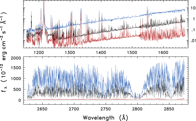
Figure 2. Overview of HST/STIS spectra of α Cen A (dark curves), α Cen B (red), and Procyon (blue). The upper panel is the FUV, from epoch-average medium-resolution spectra. The lower panel is a subsection of the NUV from epoch-average high-resolution spectra. The tracings are presented in observed flux densities, which provide a better separation between the stars.
Download figure:
Standard image High-resolution imageIn the upper panel (on a logarithmic flux scale), the downward sloping FUV continuua of the three stars dominate the appearance at the long wavelength end, while a progression of sharp emission lines becomes more prominent at the short end. The strong feature near 1215 Å is H i Lyα, which is by far the most intense emission of the FUV region of late-type stars. Note the prominent jump (toward shorter wavelengths) at the Si i photoionization edge near 1520 Å in α Cen B, but apparent absorption dip (albeit weak) at the edge in Procyon.
In the lower panel for the NUV, now on a linear scale, the depressed photospheric continuum of cooler α Cen B is conspicuous compared to bright, warmer Procyon; yet the chromospheric Mg ii hk emission peaks, which are barely visible at the bottoms of the deep photospheric Mg ii absorptions bracketing 2800 Å, are roughly the same strength in all three stars (in observed flux). The other deep absorption feature in this interval, near 2850 Å, is the Mg i 2852 Å resonance line. The Mg ii emissions appear rather uninspiring relative to their surroundings compared with, say, FUV Lyα, but in reality the combined hk core flux is several times that of the hydrogen line in all three stars.
2.4. Solar-stellar Comparison
Before describing the detailed measurements of the UV emission lines of the three STIS stars, it is instructive to show, in Figure 3, the epoch-average profiles of representative features—C ii 1334 Å, C ii 1335 Å, Si iv 1393 Å, and Mg ii 2796 Å (k)—and the solar counterparts, at similar spectral resolution, from the IRIS full-disk mosaics described in Paper IV. The upper darker curves for the Sun are averages from near the Cycle 24 peak. The lower red curves represent an average over very quiet conditions. The darker curves for α Cen B and Procyon are from epoch-average high-resolution STIS spectra. The red curves for all three stars (including α Cen A) are from epoch-average medium-resolution FUV spectra. (The NUV Mg ii k line was exclusively recorded in high resolution.) Deep interstellar absorptions appear in the low-ionization ground-state transitions C ii 1334 Å and Mg ii 2796 Å, which are sharper in high resolution than medium resolution. Of course, the solar profiles are not affected. The ISM features are more centered in the α Cen stars but significantly redshifted in Procyon, due to the differences between the stellar systemic velocities and those of the local interstellar clouds.

Figure 3. Four representative emission features of the STIS stars compared to solar equivalents from the IRIS full-disk spectra described in Paper IV. Upper darker curves for the Sun ("S") are from near the peak of Cycle 24. The lower red curves represent very quiet conditions. Darker curves in the left-hand panel for α Cen B ("B") and Procyon ("P") are from FUV-H epoch-average spectra. The red curves for the STIS stars are from FUV-M epoch averages (no FUV-H for α Cen A ("A")). The STIS Mg ii lines were exclusively observed in NUV-H. The weak emission blip at +1.5 Å from the k-line center, most evident in Procyon, lacks a convincing identification; however, it might be analogous to the rare-earth emission lines seen in the wings of the solar Ca ii HK lines near the limb (Canfield 1971).
Download figure:
Standard image High-resolution imageAdditional small differences in the ISM absorptions between α Cen A and B accrue from the relative orbital motion (most obvious in high-resolution Mg ii). Also note the tiny redshifted divot at the peak of Procyon's excited-state transition C ii 1335 Å (whose lower level is 63 cm−1 above ground). This notch must be interstellar, but the absorption is severely reduced compared to the ground-state resonance line owing to the radiative depletion of the C+ excited fine-structure population under the extremely tenuous conditions in the local interstellar gas. The reduced ISM absorption in C ii 1335 Å has revealed clear central reversals in the stars owing to high opacity, mimicking the slanted-topped peak of the solar full-disk profile (high-spatial resolution tracings of solar 1335 Å often show more obvious central dips: see Paper IV). The same story is repeated in Mg ii 2796 Å, as follows: strong central reversals in the solar profiles; somewhat obscured reversals in the α Cen stars; and a cleaner feature in Procyon, thanks to the redshifted ISM absorption. Superficially, the α Cen A and solar profiles are very similar in shape and strength; the α Cen B counterparts are narrower and stronger than solar (with the fλ /fBOL normalization); and the Procyon features are wider and stronger, most conspicuously chromospheric C ii and Mg ii. Aside from the sharp interstellar features, differences between the medium-resolution and high-resolution FUV line shapes of α Cen B and Procyon are comparatively minor.
3. Analysis
This section describes the specialized spectral fitting carried out for epoch-average and epoch-resolved UV spectra of the three STIS stars, as motivated by the experience of Paper IV. Results of the spectral fitting are presented in a series of tables and diagrams later in the section. Alpha Cen A will be utilized here as the example to illustrate the fitting procedures. Appendix C separately provides additional illustrations of the line fits for α Cen B and Procyon, especially the differences between the FUV-M and FUV-H epoch averages.
3.1. STIS Spectral Fitting
As described in the Introduction, Paper IV introduced a pseudo-Gaussian fitting model,

in which the normal pure-Gaussian exponent (a = 2) was allowed to take on arbitrary values. Here, λ0 is the line-center wavelength and ΔλD is the characteristic e-folding line width. A pure Gaussian, as has been noted in prior solar and stellar work, tends to have a shallower, broader peak, slightly bowed sides, and narrower wings than typical empirical TZ line shapes. In some previous work, the mismatch was accommodated by introducing a bimodal Gaussian model in which a broad component provided the extended line wings, while a narrow component contributed the sharper central peak. However, Paper IV demonstrated that the simple pseudo-Gaussian model could replicate a diversity of solar line shapes, including the narrow-core, broad-wing profiles of optically thin TZ lines, as well as the boxier shapes of the optically thick chromospheric features (albeit ignoring the central reversals if too prominent, as in the Mg ii features).
Figure 4 illustrates two of the main optically thin TZ lines, N v 1238 Å and Si iv 1393 Å, from the epoch-average medium-resolution spectra of the three STIS stars. These features are less affected by extraneous blends than other TZ emissions (although note the faint Ni ii feature in the blue wing of the Si iv line of Procyon). Each emission profile was fitted by a least-squares Gaussian (red) and a pseudo-Gaussian model (green; derived a exponent listed for each line; a = 2 is the pure Gaussian). Dark dots represent the observed STIS spectra. Points within the intervals marked by the blue inverted-L symbols were included in the modeling for each approximation. Horizontal blue-dashed lines depict long-range continuum fits, which were subtracted from the target flux densities prior to the profile modeling. Each observed feature was normalized to its peak intensity for display purposes: note the y-axis scales at the left and right.
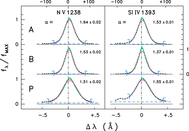
Figure 4. N v 1238 Å and Si iv 1393 Å from the epoch-average medium-resolution spectra of the three STIS stars, normalized to their intensity peaks. Each line was fitted by a least-squares Gaussian (red) and a pseudo-Gaussian model (green; derived a exponent listed for each line). The dark dots are the observed spectra. Points between the inverted-L symbols were included in each fit. Horizontal blue-dashed lines represent long-range continuum fits.
Download figure:
Standard image High-resolution imageThe pseudo-Gaussian profiles match the observed line shapes better than the pure Gaussians, which is unsurprising given the additional degree of freedom available. Perhaps more intriguing is that the derived pseudo-Gaussian exponents are similar for the two different TZ lines in each star, despite the obvious diversity in line widths; as well as similar among the stars, with values ∼1.5, significantly less than the pure-Gaussian case. (Uncertainties in the modeling were assessed by a Monte Carlo approach, in which the best-fit profile was Gaussian-perturbed point-by-point according to the local photometric errors, then refitted, in numerous independent trials. The standard deviations of the derived parameters, especially the a exponent, over the many trials was a gauge of the uncertainties.)
Paper IV further showed that the straightforward interpretation of the double-Gaussian alternative—that each component was contributed by a separate, distinct class of surface structures with different internal kinematics, which became blended in the disk average—was too simplistic because the same pseudo-Gaussian line shape of Si iv 1393 Å was seen not only in the full-disk average but also down to the finest spatial scales of the IRIS mosaics. This suggested that some widespread process was shaping the TZ lines at very fine spatial scales. One possibility mentioned was the so-called "κ-mechanism" (Dudík et al. 2017) owing to the similarity between the κ profile and the pseudo-Gaussian model for a < 2. There might be other, alternative non-Maxwellian processes that could produce the characteristic TZ line shape as well. In Paper IV, the pseudo-Gaussian modeling was preferred over the κ profile from the pragmatic point of view that the former can accommodate both the sharply peaked a < 2 TZ profiles, as well as the more rounded a > 2 line shapes of the optically thick chromospheric features; whereas, the κ profile has the limiting form of a pure Gaussian for large κ, and thus cannot access the realm inhabited by the boxier shapes of, say, the C ii and Mg ii emission cores. (The more rectangular a > 2 profiles also are inaccessible to the double-Gaussian modeling.) For that reason of generality, the pseudo-Gaussian line shape was preferred here to model the UV profiles of the three STIS stars.
The pseudo-Gaussian was implemented in an algorithm driven by parameters that were customized for each target spectral feature and each star. The emission lines were affected to varying degrees by accidental blends, whose influence varied among the stars (e.g., the Ni ii blend in Si iv in Figure 4 and the interstellar absorptions seen in Figure 3). In addition, the shapes of the target emission lines also varied among the stars (specifically the line widths). Two separate line lists were used to drive the algorithm.
The first list (Table 5) was designed to validate the velocity scales of the individual (or average) spectra, and consisted of a set of narrow low-excitation neutral chromospheric emissions for the FUV, and photospheric absorptions (in the Mg ii hk wings) for the NUV. Although careful corrections to the STIS (relative) wavelength scales were made during the initial processing steps, the absolute zero-point of an observation can be affected by the accuracy of the target centering, or by subsequent drifts and telescope breathing. Beyond that, all three STIS stars are in binary systems, so there are additional orbital velocity shifts, which vary over time. The strategy was to assume that low-excitation FUV emission lines forming in the deep chromosphere, or absorption lines in the Mg ii wings arising in the high photosphere, would have instantaneous velocities close to that of the photosphere, and thus could serve as zero-point calibrators. As a first step in the analysis, all the individual spectra, and the various M and H epoch-average versions, were adjusted in radial velocity according to the average of the respective sets of FUV or NUV reference lines. The derived values of the apparent radial velocities for the individual STIS spectra were noted previously in Table 4.
Table 5. STIS Fitting Parameters: Radial-velocity Calibrators
| Species | λLAB | συ | ELOW | Δλ (AB) | Δλ (P) |
|---|---|---|---|---|---|
| (Å) | (km s−1) | (cm−1) | (Å) | ||
| 1 | 2 | 3 | 4 | 5 | 6 |
| S i | 1300.907 | 0.2 | 9239 | (−0.100, +0.080) | (−0.080, +0.100) |
| Cl i | 1351.656 | <0.2 | 882 | ±0.110 | ±0.110 |
| O i | 1355.598 | <0.2 | 0 | (−0.110, +0.090) | ±0.110 |
| O i | 1358.512 | <0.2 | 158 | ±0.100 | ±0.090 |
| Fe i | 2788.927 | <0.2 | 6928 | ±0.100 | ±0.100 |
| Mn i | 2799.094 | 0.8 | 0 | (−0.090, +0.100) | (−0.080, +0.100) |
| Mn i | 2801.907 | 0.8 | 0 | ±0.100 | ±0.100 |
| Fe i | 2805.346 | <0.2 | 7377 | (−0.090, +0.080) | ±0.080 |
| Fe i | 2809.154 | <0.2 | 7728 | ±0.090 | ±0.090 |
| Fe i | 2814.115 | <0.2 | 7377 | (−0.080, +0.090) | ±0.090 |
Note. Col. 1 is the species name. Col. 2 is the laboratory wavelength from the Atomic Spectra Database (https://physics.nist.gov/PhysRefData/ASD/lines_form.html) of the National Institute of Standards and Technology (NIST). Col. 3 is the uncertainty in λLAB expressed in velocity units, as quoted by NIST, if available; otherwise from the Atomic Line List v.300b3 (https://www.pa.uky.edu/~peter/newpage/). Col. 4 is the lower level excitation energy. Cols. 5 and 6 are the outer wavelength bounds, relative to λLAB, for the pseudo-Gaussian modeling of AB and Procyon, respectively.
Download table as: ASCIITypeset image
In the Table 5 velocity calibrator line list, there are two sets of wavelength offsets, one for the AB lines, the other for Procyon. The offsets—which are sometimes symmetrical, but sometimes not—indicate the wavelength range relative to the laboratory value, λLAB, over which the particular profile was fitted (also using the pseudo-Gaussian model). Asymmetric offsets accommodated situations such as O i 1355 Å, where another feature (in this case a weak C i transition to the red) was close enough to affect one of the line wings.
The second line list (Table 6) was for the target emission lines of the FUV and NUV regions, including several broad continuum bands. In the NUV, as noted earlier, the continuum bands were employed to adjust the flux density scales to counter narrow-slit variable transmissions. Parameters for the three stars are tabulated in separate rows organized by line transition or continuum band. The first pair of entries in each row are wavelength bounds for an integrated flux measurement, which are asymmetric in some cases for the same reasons as given earlier for the velocity reference lines. The middle pair denotes the outer bounds of the pseudo-Gaussian fitting, as in Table 5 for the velocity calibrators. The final set of entries in the row, if present, indicates an inner wavelength interval that was ignored because of an optically thick central reversal or a sharp interstellar absorption. In what follows, the quoted fluxes of the lines will be the integrated values, encompassing a central reversal or ISM absorption if present; rather than, say, the value derived from the pseudo-Gaussian fit itself. This was done to ensure that the time histories of the fluxes were not affected by artifacts associated with the fitting process, or the over-prediction of the line intensities in the cases where central reversals were ignored.
Table 6. STIS Fitting Parameters: Stellar Emission Lines
| Species | λLAB | συ | TMAX | Cflag | Star | ΔλintF | ΔλpGfit | ΔλCrev |
|---|---|---|---|---|---|---|---|---|
| (Å) | (km s−1) | (K) | (Å) | |||||
| 1 | 2 | 3 | 4 | 5 | 6 | 7 | 8 | 9 |
| Si iii | 1206.500 | 0.3 | 4.7 | C | A | (−0.275, +0.375) | (−0.275, +0.325) | ⋯ |
| B | (−0.275, +0.375) | (−0.275, +0.325) | ⋯ | |||||
| P | (−0.475, +0.525) | (−0.375, +0.425) | (−0.100, +0.165) | |||||
| H i | 1215.670 | 0.6 | (4.3) | C | A | ±1.500 | ±1.250 | (−0.400, +0.300) |
| B | ±1.400 | ±1.200 | (−0.365, +0.280) | |||||
| P | ±1.750 | ±1.250 | (−0.400, +0.375) | |||||
| O v | 1218.344 | 3 | 5.3 | S | A | (−0.235, +0.265) | (−0.185, +0.215) | ⋯ |
| B | (−0.235, +0.265) | (−0.160, +0.190) | ⋯ | |||||
| P | (−0.385, +0.415) | (−0.235, +0.315) | ⋯ | |||||
| N v | 1238.810 a | 0.7 | 5.2 | C | A | (−0.375, +0.425) | (−0.275, +0.325) | ⋯ |
| B | (−0.375, +0.425) | (−0.275, +0.325) | ⋯ | |||||
| P | (−0.475, +0.525) | (−0.375, +0.425) | ⋯ | |||||
| Fe xii | 1241.987 b | ⋯ | 6.2 | S | A | ±0.250 | ⋯ | ⋯ |
| B | ±0.250 | ±0.200 | ⋯ | |||||
| P | ±0.250 | ⋯ | ⋯ | |||||
| N v | 1242.800 a | 0.7 | 5.2 | C | A | (−0.230, +0.270) | (−0.230, +0.270) | ⋯ |
| B | (−0.230, +0.270) | (−0.230, +0.270) | ⋯ | |||||
| P | (−0.480, +0.520) | (−0.380, +0.420) | ⋯ | |||||
| O i | 1302.168 | <0.2 | (3.9) | C | A | (−0.295, +0.305) | (−0.245, +0.255) | (−0.055, +0.065) |
| B | (−0.220, +0.230) | (−0.195, +0.205) | (−0.040, +0.060) | |||||
| P | (−0.345, +0.355) | (−0.295, +0.305) | (−0.070, +0.170) | |||||
| O i | 1304.858 | <0.2 | (3.9) | C | A | ±0.275 | ±0.200 | ±0.060 |
| B | ±0.225 | ±0.200 | ±0.050 | |||||
| P | ±0.300 | ±0.250 | (−0.065, +0.070) | |||||
| O i | 1306.029 | <0.2 | (3.9) | C | A | ±0.275 | ±0.200 | ⋯ |
| B | ±0.225 | ±0.200 | ⋯ | |||||
| P | ±0.300 | ±0.250 | ±0.050 | |||||
| C ii | 1334.532 | 0.4 | 4.5 | C | A | (−0.390, +0.410) | (−0.290, +0.310) | (−0.055, +0.070) |
| B | (−0.390, +0.410) | (−0.290, +0.310) | (−0.065, +0.085) | |||||
| P | (−0.490, +0.510) | (−0.390, +0.410) | (−0.090, +0.185) | |||||
| C ii | 1335.702 | 0.4 | 4.5 | C | A | (−0.345, +0.405) | (−0.295, +0.305) | ±0.060 |
| B | (−0.395, +0.405) | (−0.295, +0.305) | (−0.050, +0.055) | |||||
| P | (−0.345, +0.505) | (−0.295, +0.405) | (−0.120, +0.130) | |||||
| Fe xii | 1349.397 b | ⋯ | 6.2 | C | A | ±0.250 | ⋯ | ⋯ |
| B | ±0.250 | ±0.200 | ⋯ | |||||
| P | ±0.250 | ⋯ | ⋯ | |||||
| Cl i | 1351.656 | <0.2 | (3.8) | C | A | (−0.130, +0.120) | (−0.130, +0.120) | ⋯ |
| B | (−0.130, +0.120) | (−0.130, +0.120) | ⋯ | |||||
| P | (−0.155, +0.145) | (−0.155, +0.145) | ⋯ | |||||
| O i | 1355.598 | <0.2 | (3.9) | C | A | (−0.130, +0.120) | (−0.130, +0.120) | ⋯ |
| B | (−0.130, +0.120) | (−0.130, +0.120) | ⋯ | |||||
| P | (−0.155, +0.145) | (−0.155, +0.145) | ⋯ | |||||
| Si iv | 1393.760 a | <0.2 | 4.9 | C | A | (−0.280, +0.520) | (−0.230, +0.420) | ⋯ |
| B | (−0.280, +0.420) | (−0.280, +0.320) | ⋯ | |||||
| P | (−0.280, +0.520) | (−0.230, +0.420) | ⋯ | |||||
| O iv | 1401.164 c | 3 | 5.1 | C | A | (−0.330, +0.270) | (−0.230, +0.220) | ⋯ |
| B | (−0.330, +0.270) | (−0.230, +0.220) | ⋯ | |||||
| P | (−0.280, +0.320) | (−0.230, +0.270) | ⋯ | |||||
| Si iv | 1402.773 a | <0.2 | 4.9 | C | A | (−0.385, +0.415) | (−0.285, +0.315) | ⋯ |
| B | (−0.385, +0.415) | (−0.285, +0.315) | ⋯ | |||||
| P | (−0.485, +0.515) | (−0.385, +0.415) | ⋯ | |||||
| c1506 | 1506.000 | ⋯ | (3.8) | N | A | ±2.500 | ⋯ | ⋯ |
| B | ±2.500 | ⋯ | ⋯ | |||||
| P | ±2.500 | ⋯ | ⋯ | |||||
| C iv | 1548.204 a | 0.2 | 5.0 | C | A | ±0.375 | ±0.325 | ⋯ |
| B | ±0.375 | (−0.275, +0.325) | ⋯ | |||||
| P | ±0.375 | (−0.275, +0.325) | ⋯ | |||||
| C iv | 1550.771 a | 0.4 | 5.0 | C | A | (−0.325, +0.350) | (−0.275, +0.300) | ⋯ |
| B | (−0.325, +0.350) | (−0.275, +0.300) | ⋯ | |||||
| P | ±0.375 | ±0.325 | ⋯ | |||||
| c2780 | 2780.000 | ⋯ | (3.7) | N | A | ±4.000 | ⋯ | ⋯ |
| B | ±4.000 | ⋯ | ⋯ | |||||
| P | ±4.000 | ⋯ | ⋯ | |||||
| Mg ii | 2796.352 | 0.8 | (3.9) | C | A | ±0.550 | ±0.550 | (−0.200, +0.180) |
| B | ±0.550 | ±0.550 | ±0.150 | |||||
| P | ±0.650 | ±0.650 | (−0.290, +0.325) | |||||
| Mg ii | 2803.531 | 0.8 | (3.9) | C | A | ±0.500 | ±0.500 | (−0.185, +0.180) |
| B | ±0.500 | ±0.500 | (−0.130, +0.140) | |||||
| P | ±0.600 | ±0.600 | (−0.275, +0.315) | |||||
| c2820 | 2820.000 | ⋯ | (3.7) | N | A | ±4.000 | ⋯ | ⋯ |
| B | ±4.000 | ⋯ | ⋯ | |||||
| P | ±4.000 | ⋯ | ⋯ | |||||
Notes. Col. 1 is the species name. Col. 2 is the laboratory wavelength, mainly from NIST, unless otherwise noted. Col. 3 is the uncertainty in λLAB expressed in velocity units (mostly from the Atomic Line List v.300b3). Col. 4 is the temperature of maximum emissivity in collisional ionization equilibrium (CIE) from CHIANTI (see: https://www.chiantidatabase.org/chianti_linelist.html); parenthetical values are estimates for chromospheric or photospheric features. Col. 5 is a flag for the continuum fit: C = flat; S = sloping; N = no continuum subtraction. Col. 6 indicates the star (A = α Cen A; B = α Cen B; P = Procyon). Col. 7 lists the wavelength bounds for the line profile flux integration; Col. 8, the outer wavelength limits for the pseudo-Gaussian modeling; and Col. 9, the inner limits to exclude a central reversal, if warranted.
a From Ayres (2015b), based on contemporary accurate laboratory measurements of the Si iv doublet, transferred to N v and C iv via precise relative wavelengths in STIS spectra of white dwarfs. b Empirical value, derived from the high-S/N medium-resolution epoch-average FUV spectrum of α Cen B. Measurement error ≲0.5 km s−1; absolute error uncertain owing to possible systemic coronal velocity shifts. c From Atomic Line List v.300b3: NIST value is 7 mÅ (1.5 km s−1) smaller.For practical numerical reasons, the least-squares pseudo-Gaussian fitting algorithm restricted the exponent a to the range 1–5, which accommodated the vast majority of the STIS profile shapes. Only the broad Lyα feature, which is severely truncated in its core by interstellar absorption, encroached on the boundaries of the restricted a range, in that case on the low side (a = 1 is a pure exponential).
Figure 5 illustrates the profile fitting approach applied to the epoch-average STIS spectrum of α Cen A (additional examples for α Cen B and Procyon can be found in Appendix C). Each panel depicts one of the 24 emission lines or broad continuum bands from Table 6. For all the features, flux densities were numerically integrated over the wavelength bandpasses marked in green. Blue-dashed lines under the emission features are long-range continuum fits 6 that were subtracted prior to the fitting procedure (not applied to the continuum bands). In the cases of O v 1218 Å and coronal forbidden line Fe xii 1241 Å, the continuum fits were allowed to be tilted, or curved, to account for the wings of nearby stronger emissions: Lyα and N v 1242 Å, respectively. (Here, the outcome is more noticeable for O v.) Most of the emission lines then were subjected to the pseudo-Gaussian modeling, taking target flux densities between the outer blue inverted-L symbols, and, in cases of strong central reversals or ISM absorptions, ignoring the points between the inner inverted-Ls. For α Cen A, here, and Procyon later (in Appendix C), both of the faint Fe xii coronal forbidden lines were too noisy to be reliably fitted by a pseudo-Gaussian. In contrast, the Fe xii features of α Cen B were much stronger thanks to the higher intensity corona of the K dwarf, and thus were able to be successfully modeled.

Figure 5. Illustration of the profile fitting approach applied to the epoch-average STIS spectrum of α Cen A. Each panel depicts one of the 24 emission lines or broad continuum bands that were considered. For all of the features, flux densities were numerically integrated over the wavelength bandpasses marked in green. "Inverted-L" symbols delimit the points included in the pseudo-Gaussian modeling. Blue-dashed lines under the emission features are long-range continuum fits.
Download figure:
Standard image High-resolution imageThe Mg ii hk lines were a special case. A minimum wing intensity (highlighted by a yellow dot) was determined in a slightly smoothed version of the local spectrum in a narrow band (marked by vertical orange tics) on whichever side of the k or h line that was least affected by blends. This baseline flux density was subtracted from the k or h profile prior to fitting, in the same way as the background continuum was compensated in the more general case. The difference here is that some fraction of the Mg ii flux under the baseline represents legitimate chromospheric emission, because without a chromosphere the line cores would be deep, broad U-shaped absorption features (see Linsky & Ayres 1978). These absorption cores then are filled-in to varying degrees by chromospheric emission, depending on the activity level. Nevertheless, the adopted background-subtraction approach for Mg ii was expedient, avoiding overestimating the hk flux if instead the flux integration were done without the subtraction (i.e., integrating all the flux densities above zero between the local minimum features); and further avoiding a challenging correction to establish the exact proportion of the "block flux" under the Mg ii minima that truly is chromospheric. The same scheme was applied to Mg ii in the Sun and α Cen AB in Paper I, with good results. Namely, the background-subtracted hk fluxes displayed tight correlations with other chromospheric tracers, such as the O i 1305 Å triplet and the C ii 1335 Å multiplet. At the same time, the k and h block fluxes (c2796 and c2803, respectively), which were retained separately, also showed good correlations with legitimate chromospheric diagnostics but with much shallower slopes than the corresponding Mg ii core fluxes, as anticipated if a chromospheric contribution is present but is relatively minor.
Table 7 summarizes the line shape parameters and bolometrically normalized fluxes measured in the FUV-M and NUV-H epoch-average spectra of the three stars, again presented in separate rows. Also included are MAX/MIN flux contrasts (defined as  in percents based on the time-resolved spectra). The leading uncertainties provided on the profile shape parameters are 1σ measurement errors (related to the S/N), while the following parenthetical values are 1σ standard deviations over the available epochs, excluding the two most extreme outliers in each series, probing variability of the respective quantities over the stellar activity cycles (or a more quiescent period, as was the case for Procyon).
Table 7. STIS Stellar Emission Line Parameters: Epoch-average Spectra and Time-series Variability
| Species | Star | υ ± συ | FWHM ± σFW | a ± σa | fL/fBOL | fC/fBOL |
|---|---|---|---|---|---|---|
| (km s−1) | (10−7) (%) | (10−7 Å−1) | ||||
| 1 | 2 | 3 | 4 | 5 | 6 | 7 |
| Si iii 1206 | A | +5.6 ± 0.1 (0.2) | 58.8 ± 0.2 (0.7) | 2.01 ± 0.02 (0.03) | 0.71 (34) | 0.00 |
| B | +4.7 ± 0.1 (0.3) | 45.8 ± 0.2 (2.0) | 1.71 ± 0.01 (0.06) | 1.08 (86) | 0.00 | |
| P | +5.0 ± 0.1 (0.3) | 77.2 ± 1.2 (3.0) | 1.71 ± 0.03 (0.06) | 2.42 (7) | 0.00 | |
| H i 1215 | A | +0.4 ± 0.1 (0.2) | 61.7 ± 0.3 (0.5) | 1.00 ± 0.00 (0.00) | 18.9 (19) | 0.052 |
| B | −0.2 ± 0.1 (0.3) | 57.7 ± 0.2 (0.8) | 1.00 ± 0.00 (0.00) | 51 (58) | 0.085 | |
| P | −5.6 ± 0.1 (0.3) | 79.1 ± 0.5 (0.8) | 1.00 ± 0.00 (0.00) | 26.0 (9) | 0.159 | |
| O v 1218 | A | +4.1 ± 0.3 (1.1) | 55.8 ± 0.9 (3.5) | 1.73 ± 0.08 (0.23) | 0.108 (33) | 0.078 |
| B | +2.6 ± 0.2 (0.8) | 46.3 ± 0.7 (3.1) | 1.74 ± 0.07 (0.24) | 0.175 (125) | 0.131 | |
| P | +6.7 ± 0.3 (0.6) | 68.8 ± 1.0 (3.3) | 1.48 ± 0.05 (0.10) | 0.35 (24) | 0.33 | |
| N v 1238 | A | +5.2 ± 0.1 (0.3) | 51.1 ± 0.4 (2.0) | 1.64 ± 0.02 (0.08) | 0.107 (24) | 0.0109 |
| B | +3.5 ± 0.1 (0.3) | 42.3 ± 0.3 (2.3) | 1.53 ± 0.02 (0.10) | 0.219 (128) | 0.0101 | |
| P | +7.0 ± 0.1 (0.4) | 71.2 ± 0.5 (1.4) | 1.51 ± 0.02 (0.04) | 0.49 (8) | 0.066 | |
| Fe xii 1241 | A | ⋯ | ⋯ | ⋯ | 0.0047 (309) | 0.0106 |
| B | −0.0 ± 0.3 (1.1) | 44.5 ± 0.8 (5.6) | 1.84 ± 0.08 (0.48) | 0.0258 (140) | 0.0119 | |
| P | ⋯ | ⋯ | ⋯ | 0.0068 (124) | 0.077 | |
| N v 1242 | A | +5.1 ± 0.2 (0.2) | 52.6 ± 0.5 (2.0) | 1.76 ± 0.04 (0.11) | 0.052 (19) | 0.0088 |
| B | +2.8 ± 0.1 (0.8) | 43.1 ± 0.3 (2.3) | 1.63 ± 0.02 (0.09) | 0.106 (116) | 0.0103 | |
| P | +6.9 ± 0.2 (0.3) | 69.6 ± 0.6 (1.6) | 1.41 ± 0.02 (0.03) | 0.260 (8) | 0.063 | |
| O i 1302 | A | +0.9 ± 0.1 (0.1) | 38.4 ± 0.4 (1.6) | 1.97 ± 0.03 (0.09) | 0.260 (20) | 0.0082 |
| B | +0.1 ± 0.1 (0.3) | 35.0 ± 0.2 (2.3) | 1.97 ± 0.02 (0.09) | 0.45 (70) | 0.0087 | |
| P | +0.7 ± 0.1 (0.2) | 58.9 ± 0.5 (1.8) | 2.31 ± 0.04 (0.11) | 0.63 (10) | 0.133 | |
| O i 1304 | A | −0.2 ± 0.1 (0.1) | 40.8 ± 0.3 (1.5) | 2.35 ± 0.03 (0.12) | 0.31 (16) | 0.0099 |
| B | −0.4 ± 0.1 (0.4) | 30.4 ± 0.4 (2.8) | 1.83 ± 0.03 (0.11) | 0.55 (76) | 0.0094 | |
| P | +0.8 ± 0.1 (0.4) | 57.3 ± 0.3 (1.3) | 2.65 ± 0.04 (0.07) | 0.75 (11) | 0.147 | |
| O i 1306 | A | −0.3 ± 0.1 (0.1) | 39.6 ± 0.1 (0.6) | 2.46 ± 0.01 (0.07) | 0.34 (15) | 0.0071 |
| B | −0.5 ± 0.1 (0.3) | 32.9 ± 0.1 (1.1) | 2.17 ± 0.01 (0.15) | 0.58 (67) | 0.0052 | |
| P | +0.8 ± 0.1 (0.2) | 45.5 ± 0.3 (1.8) | 1.97 ± 0.02 (0.05) | 0.83 (9) | 0.131 | |
| C ii 1334 | A | +1.9 ± 0.1 (0.2) | 44.7 ± 0.3 (1.1) | 1.85 ± 0.01 (0.05) | 0.46 (19) | 0.0095 |
| B | +1.3 ± 0.1 (0.2) | 24.0 ± 0.4 (4.1) | 1.25 ± 0.02 (0.12) | 0.77 (74) | 0.0065 | |
| P | +2.6 ± 0.1 (0.1) | 56.0 ± 0.6 (1.5) | 1.57 ± 0.02 (0.04) | 1.72 (7) | 0.176 | |
| C ii 1335 | A | +1.2 ± 0.1 (0.1) | 55.7 ± 0.2 (0.9) | 2.14 ± 0.01 (0.05) | 0.73 (19) | 0.0093 |
| B | +0.8 ± 0.1 (0.2) | 45.1 ± 0.1 (2.2) | 1.88 ± 0.01 (0.09) | 1.37 (79) | 0.0059 | |
| P | +2.2 ± 0.1 (0.2) | 76.1 ± 0.5 (2.9) | 2.02 ± 0.02 (0.07) | 2.40 (8) | 0.183 | |
| Fe xii 1349 | A | ⋯ | ⋯ | ⋯ | 0.0019 (221) | 0.0109 |
| B | +0.1 ± 0.4 (1.2) | 46.9 ± 1.1 (5.2) | 2.05 ± 0.15 (0.50) | 0.0114 (107) | 0.0066 | |
| P | ⋯ | ⋯ | ⋯ | 0.0034 (175) | 0.204 | |
| Cl i 1351 | A | −0.1 ± 0.1 (0.1) | 17.6 ± 0.2 (0.4) | 1.78 ± 0.03 (0.05) | 0.047 (15) | 0.0111 |
| B | −0.2 ± 0.1 (0.2) | 15.6 ± 0.1 (2.8) | 1.73 ± 0.03 (0.11) | 0.054 (68) | 0.0067 | |
| P | −0.1 ± 0.1 (0.2) | 22.1 ± 0.1 (1.9) | 1.82 ± 0.02 (0.04) | 0.240 (13) | 0.208 | |
| O i 1355 | A | −0.4 ± 0.1 (0.1) | 17.3 ± 0.1 (0.5) | 1.68 ± 0.02 (0.05) | 0.070 (8) | 0.0127 |
| B | −0.4 ± 0.1 (0.3) | 15.5 ± 0.1 (2.7) | 1.61 ± 0.02 (0.11) | 0.084 (34) | 0.0079 | |
| P | −0.0 ± 0.1 (0.1) | 20.0 ± 0.2 (1.6) | 1.54 ± 0.02 (0.05) | 0.176 (11) | 0.215 | |
| Si iv 1393 | A | +3.8 ± 0.1 (0.2) | 44.3 ± 0.2 (0.7) | 1.53 ± 0.01 (0.03) | 0.36 (32) | 0.0179 |
| B | +2.7 ± 0.1 (0.4) | 35.2 ± 0.1 (1.5) | 1.37 ± 0.01 (0.04) | 0.61 (97) | 0.0107 | |
| P | +5.1 ± 0.1 (0.3) | 65.3 ± 0.2 (0.9) | 1.55 ± 0.01 (0.02) | 1.15 (19) | 0.32 | |
| O iv 1401 | A | +4.9 ± 0.2 (0.5) | 43.9 ± 0.6 (2.7) | 1.56 ± 0.05 (0.20) | 0.038 (18) | 0.0210 |
| B | +3.2 ± 0.2 (0.9) | 38.6 ± 0.5 (3.4) | 1.60 ± 0.04 (0.16) | 0.049 (66) | 0.0132 | |
| P | +7.2 ± 0.3 (0.7) | 57.5 ± 0.8 (2.5) | 1.53 ± 0.06 (0.12) | 0.164 (28) | 0.34 | |
| Si iv 1402 | A | +3.9 ± 0.1 (0.4) | 42.9 ± 0.3 (0.9) | 1.50 ± 0.01 (0.03) | 0.188 (31) | 0.0202 |
| B | +3.0 ± 0.1 (0.3) | 34.8 ± 0.2 (1.8) | 1.37 ± 0.01 (0.06) | 0.32 (91) | 0.0120 | |
| P | +4.4 ± 0.1 (0.4) | 61.3 ± 0.4 (1.4) | 1.44 ± 0.02 (0.03) | 0.63 (22) | 0.35 | |
| c1506 | A | ⋯ | ⋯ | ⋯ | 0.265 (8) | ⋯ |
| B | ⋯ | ⋯ | ⋯ | 0.136 (51) | ⋯ | |
| P | ⋯ | ⋯ | ⋯ | 4.1 (18) | ⋯ | |
| C iv 1548 | A | +4.7 ± 0.1 (0.2) | 51.2 ± 0.2 (0.9) | 1.58 ± 0.01 (0.04) | 0.72 (23) | 0.055 |
| B | +2.9 ± 0.1 (0.4) | 41.1 ± 0.1 (1.0) | 1.47 ± 0.01 (0.05) | 1.25 (91) | 0.0192 | |
| P | +6.7 ± 0.1 (0.3) | 75.9 ± 0.2 (0.9) | 1.93 ± 0.02 (0.05) | 2.78 (12) | 1.36 | |
| C iv 1550 | A | +5.1 ± 0.1 (0.3) | 51.9 ± 0.3 (0.8) | 1.69 ± 0.02 (0.04) | 0.36 (23) | 0.061 |
| B | +2.9 ± 0.1 (0.7) | 41.6 ± 0.2 (2.1) | 1.56 ± 0.01 (0.08) | 0.62 (88) | 0.0194 | |
| P | +4.6 ± 0.1 (0.8) | 63.8 ± 0.4 (1.6) | 1.37 ± 0.02 (0.07) | 1.41 (14) | 1.45 | |
| c2780 | A | ⋯ | ⋯ | ⋯ | 910 (–) | ⋯ |
| B | ⋯ | ⋯ | ⋯ | 273 (–) | ⋯ | |
| P | ⋯ | ⋯ | ⋯ | 3258 (–) | ⋯ | |
| c2796 | A | ⋯ | ⋯ | ⋯ | 20.8 (4) | ⋯ |
| B | ⋯ | ⋯ | ⋯ | 9.1 (9) | ⋯ | |
| P | ⋯ | ⋯ | ⋯ | 81 (7) | ⋯ | |
| Mg ii 2796 | A | −1.5 ± 0.1 (0.1) | 63.4 ± 0.1 (0.3) | 3.29 ± 0.02 (0.08) | 62 (13) | 18.9 |
| B | −0.6 ± 0.1 (0.1) | 54.7 ± 0.1 (0.6) | 2.77 ± 0.01 (0.05) | 116 (46) | 8.2 | |
| P | −2.6 ± 0.1 (0.2) | 84.6 ± 0.6 (2.9) | 3.14 ± 0.06 (0.24) | 83 (6) | 62 | |
| c2803 | A | ⋯ | ⋯ | ⋯ | 22.5 (4) | ⋯ |
| B | ⋯ | ⋯ | ⋯ | 10.0 (8) | ⋯ | |
| P | ⋯ | ⋯ | ⋯ | 91 (9) | ⋯ | |
| Mg ii 2803 | A | −1.5 ± 0.1 (0.1) | 57.0 ± 0.2 (0.7) | 3.32 ± 0.03 (0.10) | 42 (14) | 22.5 |
| B | −0.2 ± 0.1 (0.1) | 52.0 ± 0.1 (0.3) | 3.02 ± 0.01 (0.04) | 81 (48) | 10.0 | |
| P | −3.1 ± 0.1 (0.3) | 76.1 ± 0.6 (4.0) | 3.32 ± 0.09 (0.34) | 49 (14) | 75 | |
| c2820 | A | ⋯ | ⋯ | ⋯ | 1330 (–) | ⋯ |
| B | ⋯ | ⋯ | ⋯ | 396 (–) | ⋯ | |
| P | ⋯ | ⋯ | ⋯ | 4684 (–) | ⋯ | |
Note. Col. 1 is the species name. Col. 2 indicates the star (A = α Cen A; B = α Cen B; P = Procyon) for the epoch-average spectrum (FUV-M and NUV-H versions). Col. 3 is the velocity shift of the species relative to the RV set by narrow, low-excitation lines. The parenthetical value is the "epoch standard deviation" (ESD), the rms variation over all the epochs, including both M and H resolutions, and excluding two outliers. Col. 4 is the derived line width expressed in velocity units, with the associated parenthetical ESD. Col. 5 is the fitted pseudo-Gaussian exponent, also with the ESD (a values were restricted by the fitting algorithm to the range 1–5; H i Lyα systematically bottomed out at the lower limit for all three stars). Col. 6 is the normalized integrated line flux. Here, the italicized parenthetical value is the flux contrast (high/low − 1) in percents. Col. 7 is the associated background continuum level at line center (in some cases the fitted continuum was tilted), expressed in flux density units divided by the bolometric flux. The sum of the continuum bands c2780 and c2820 was used to scale the NUV fluxes, to counteract variable narrow-slit throughputs; so the ESD for these two bands is artificially zero.
Figure 6 is a super-summary of the integrated UV flux measurements of the three STIS stars and the Sun, also including the broadband X-rays. Error bars on AB's X-rays were determined by 0.3 ks parsings of the Chandra event lists (∼1.5–3 hr total duration each) including any flare excursions (so far only clearly recognized in α Cen B), whereas the flares were intentionally filtered out for the mean values. Error bars for ostensibly constant Procyon were simple Poisson  . Each time series was normalized to an average flux, fAVE, as determined from the time interval outlined by vertical dotted–dashed lines in each panel (possibly different for the X-rays, and Mg ii of α Cen A, compared with the FUV). The selected intervals were intended to encompass a local cycle minimum of the time series, or as close to a minimum as practical. The normalization was according to fL/fAVE − 1. In the Chandra X-ray series, a 2% per year sensitivity decline of the HRC-I camera since 2010 was compensated. That decrease is roughly compatible with predictions by the exposure time calculator WebPIMMS, and entirely flattens the Procyon coronal time series.

Figure 6. Summary of the integrated flux measurements of the three STIS stars and the Sun, including broadband X-rays. Each time series was normalized to an average flux as determined from the time interval outlined by vertical dotted–dashed lines in each panel, intended to encompass, if possible, a local cycle minimum. The Sun and α Cen AB display excursions of their integrated fluxes that generally follow the (much larger) changes in coronal X-rays, and the amplitudes tend to increase with formation temperature (from bottom to top in each panel). In contrast, Procyon is strikingly constant in all the species, regardless of formation temperature.
Download figure:
Standard image High-resolution imageThe other emissions of Procyon that were recorded independently by STIS, with its own sensitivity variation model, show very stable long-term behavior; aside from perhaps the Fe xii coronal forbidden line, 7 which is weak and has lower S/N than the more prominent subcoronal emissions. The three Sun-like stars, excluding Procyon, display excursions of their integrated fluxes that generally follow the (much larger) changes in coronal X-rays, and the amplitudes generally increase with formation temperature (from bottom to top in each panel). Figure 6 further emphasizes the remarkable long-term stability of subgiant Procyon across the broad temperature range spanned by its corona and subcoronal atmosphere, despite its rather respectable super-solar LX/LBOL.
3.2. Correlations Among the Fitted Line Shape Parameters
The following diagrams compare different aspects of the emission-line profile shapes, separated according to low-temperature chromospheric species (T < 2 × 10⁴ K) and high-temperature TZ species (T > 5 × 10⁴ K). The representatives of the chromosphere are: O i 1306 Å ("O1306" in the figure legends); Cl i 1351 Å (Cl1351); C ii 1335 Å (C1335); and Mg ii 2796 Å (Mg2796). The TZ representatives are: Si iii 1206 Å (Si1206); N v 1238 Å (N1238); Si iv 1393 Å (Si1393); and C iv 1548 Å (C1548).
Figures 7(a) and (b) pit the pseudo-Gaussian exponent a against the e-folding line width, ΔλD as in Equation (1), for the two temperature classes, and include all the available measurements of the three STIS stars regardless of FUV resolution mode, M or H (all the NUV spectra were H). The e-folding line width appears here instead of the more common FWHM because there is already a built-in correlation between FWHM and the pseudo-Gaussian a factor:

so the e-folding width is, in some sense, more fundamental (although both, of course, are interchangeable).

Figure 7. Variation of pseudo-Gaussian exponent a as a function of profile e-folding width ΔλD for the three STIS stars, from the FUV-M, FUV-H, and NUV-H time series. Diagrams are divided into sub-Gaussian (lower, light) and super-Gaussian (upper, gray) zones. (a) Low-ionization chromospheric lines. (b) More highly ionized TZ species.
Download figure:
Standard image High-resolution imageFigure 7(a) is for the low-temperature group. The individual species are color-coded as in the upper left-hand legend. The STIS stars are represented by different symbols according to the legend at the lower right. Error bars on the individual epoch-resolved measurements are ±1σ. The diagram illustrates systematic correlations among the line shape parameters with increasing opacity: Cl1351 → O1306 → C1335 → Mg2796. Namely, the line widths increase, and the shapes evolve from sub-Gaussian (sharper cores) for the lower opacity species to super-Gaussian (boxy cores) for the optically thickest. Also note the two distinct clusters of Cl1351 points for α Cen B and Procyon, which is an influence of the M and H resolution difference and is most conspicuous in the thinnest line (both in optical depth and e-folding width). (Recall that α Cen A was observed exclusively in medium resolution, so there is no double clustering of its Cl1351 points.) A similar separation is seen in the O1306 lines of α Cen B and Procyon, and in C1335 of α Cen B (less obvious for Procyon). Furthermore, several of the species display tilted correlations between a and ΔλD, suggesting that the profiles become more rounded as they become broader. Finally, there is a general increase in the line widths α Cen B → α Cen A → Procyon, as noted earlier in Figure 3.
Figure 7(b) is for the high-temperature group, again with color-coding for the emission species and symbol-coding for the STIS stars. In contrast to the previous figure, here almost all the line shapes are sub-Gaussian, with only α Cen A's Si1206 encroaching slightly into super-Gaussian territory. Among the species illustrated, Si1206 is most likely to be optically thick—all of the others are more likely to be thin. There is not as clear a separation among the species of a given star in terms of line width but rather the strong separation by star is still maintained, with α Cen B displaying the narrowest lines and Procyon the widest. Furthermore, most of the species show relatively constant widths over a small range of measured a values, although the Si1206 trend for Procyon is noticeably tilted in the same sense as C1335 previously in Figure 7(a)—namely, the profiles become more rounded as their widths increase.
Figures 8(a) and (b) are similar to Figure 7 but now for the FWHM versus normalized line strength fL/fBOL (which is a proxy for cycle phase, at least for α Cen AB). Figure 8(a) is for the low-temperature species (same legends as Figure 7(a)). Here, the distinct lines are arrayed in flux in the same opacity pattern as previously: Cl1351 the thinnest and lowest in flux; Mg2796 the thickest and highest in flux. Across all of the stars, the average line width of a species generally increases with increasing average line strength. However, within the time series of a given species, there is a suggestion that the widths decrease with increasing line strength, especially for α Cen B; although the series for Procyon displays an insignificant variation in line fluxes, but a modest dispersion in measured line widths (the dispersion might reflect mainly measurement errors). The same M versus H separation in the FUV line widths for α Cen B is present here (and for Procyon as well), which might be biasing the suggested negative trend. However, the FUV-M and FUV-H spectra were fairly evenly distributed across the recent peaks and valleys of B's cycle.
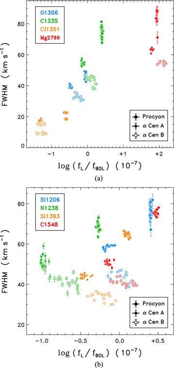
Figure 8. Variation of FWHM vs. normalized line flux for the three STIS stars, taken from the FUV-M, FUV-H, and NUV-H time series. (a) Low-ionization chromospheric lines. (b) More highly ionized TZ species.
Download figure:
Standard image High-resolution imageFigure 8(b) is for the hotter lines. Here, the widths are strongly clustered according to the star: α Cen B has the narrowest lines; Procyon the widest; with α Cen A in between. Now, the trend of decreasing line width with increasing line strength is more pronounced, at least for α Cen B, which has a much larger contrast in the line intensities over its cycle than α Cen A. The dichotomy between M and H spectra in the previous figure is less apparent because the TZ lines tend to be broader than their chromospheric cousins, at least when compared to Cl1351 and O1306. Again, the Procyon widths display a modest variation, which is more or less consistent with the measurement errors, while the line fluxes are essentially constant.
The next set of diagrams, Figure 9, depict line shifts versus normalized fluxes, again separated into chromospheric and TZ species. Figure 9(a) is for the low-temperature lines. Cl1351 clusters around zero for all of the stars, which was expected because it was one of the four narrow chromospheric emissions that established the radial-velocity normalization for each FUV spectrum. The O1306 feature is also close to zero for the α Cen stars, but moves into slightly positive territory for Procyon. C1335 displays a small redshift in all of the stars, while Mg2796 is slightly blueshifted, more so for Procyon but less so for α Cen B. Significantly, the same opposing behavior of redshifted C ii and blueshifted Mg ii was seen in spatially resolved full-disk images of the quiet Sun, which were derived from one of the IRIS mosaics in Paper IV (see Figures B1(a) and (b) therein).
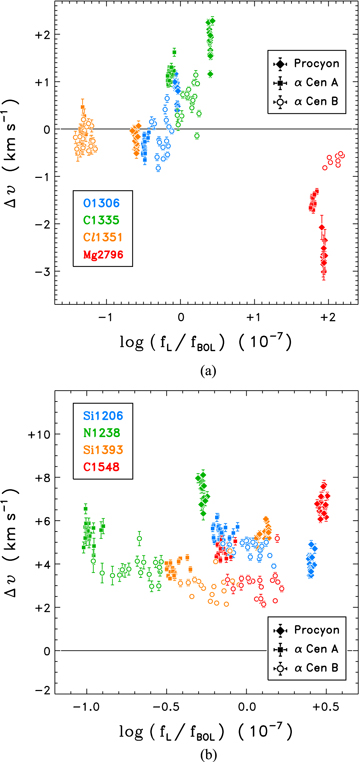
Figure 9. Variation of the line centroid velocity, calibrated against narrow chromospheric emissions (FUV) or photospheric absorptions (NUV), vs. the normalized line flux for the three STIS stars, taken from the FUV-M, FUV-H, and NUV-H time series. (a) Low-ionization chromospheric lines. (b) More highly ionized TZ species.
Download figure:
Standard image High-resolution imageFigure 9(b) is the analogous comparison for the hot lines. The appearance is entirely different than Figure 9(a), with all of the species displaying significant redshifts; less so for α Cen B, and more so for Procyon, in order of decreasing surface gravity. Within a given species, there is little apparent dependence of the shifts on the line intensities, especially in the α Cen B time series, which display the largest line-to-line flux contrasts from cycle MIN to MAX. Again, Procyon exhibits a dispersion of centroid values, which is more or less consistent with the measurement errors, over a narrow range of normalized fluxes.
Figure 10 summarizes the Doppler shift behavior of the low-temperature and high-temperature species together, arrayed as a function of formation temperature. Since there was little dependence of the line shifts on the fluxes, the highest S/N epoch-average spectra of each STIS star were appropriated for the purpose (FUV-M and NUV-H). Furthermore, many of the species illustrated in the previous figures were part of a multiplet. Now, both major members are shown (ordered in increasing wavelength from left to right in each shaded block). In addition, several new species appear, such as O i 1355 Å (which is another of the narrow chromospheric RV calibrators) and O v 1218 Å (which is the hottest of the high-S/N TZ lines, at least in CIE).
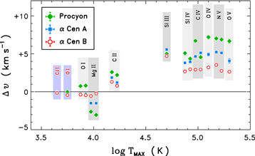
Figure 10. Line centroid velocity, calibrated relative to narrow chromospheric emissions (FUV) or photospheric absorptions (NUV), vs. formation temperature for the three STIS stars, as taken from high-S/N epoch-average spectra: FUV-M and NUV-H.
Download figure:
Standard image High-resolution imageThe two purple shaded bars at the left-hand side of the diagram are for Cl i 1351 Å and O i 1355 Å. The O i features illustrated just to the right, in the gray-shaded band, are 1304 Å and 1306 Å, which are the two members of the oxygen triplet least affected by ISM absorption. The other species in the diagram are self-explanatory. As described previously, Mg ii displays a small blueshift in all the stars, now in both spectral components, and C ii a small redshift, also in both members. The hotter TZ species mostly show a smooth change in their redshifts from Si iii temperatures (5 × 10⁴ K) up to O v (∼2 × 10⁵ K). An exception is Procyon's C iv 1550 Å, which displays a dramatically smaller redshift than the stronger member of the doublet. Examination of the epoch-average FUV-M and FUV-H spectra of Procyon (Figures C2(a) and (b), in the Appendix) finds an oddly enhanced blue wing on the 1550 Å component, which is probably caused by an unrecognized blend, and apparently pulls the line centroid slightly toward the blue. A similar distortion is not obvious in the 1550 Å features of either α Cen A or B. The Procyon spectrum is characterized by a more dominant FUV continuum than the other stars and a different set of prominent low-temperature species (e.g., numerous Ni ii transitions). Ignoring the minor distraction of 1550 Å, it is clear from Figure 10 that all three STIS stars display similar velocity profiles through the TZ, ostensibly peaking near  , but could equally be constant through that region given the uncertainties in the laboratory wavelengths of several of the lines—especially O iv, which is an intersystem transition, and O v, which is an intercombination line; both of which are difficult to measure in the laboratory.
There have been numerous reports of Doppler shifts of FUV (and EUV) TZ, and cooler, lines in the Sun. Among the studies most relevant to the present work, Hassler et al. (1991) found that the downflows in C iv 1548 Å—measured by a sounding rocket that obtained center-to-limb spectra wavelength-calibrated in flight by an onboard Pt lamp—were dominantly radial and had a peak velocity of nearly +8 km s−1 at disk center. Furthermore, C iv showed the prominent emission ring at the extreme limb described in Paper IV for similar temperature Si iv. Cooler chromospheric lines in the sounding-rocket spectra, such as Fe ii and Si ii, displayed velocities closer to zero, as did hotter Ne viii 770 Å (T ∼ 6 × 10⁵ K), the latter observed in the second order of the grating together with first-order C iv. A second pertinent study was conducted by Brekke (1999), who summarized several previous investigations. He proposed that the solar redshifts at disk center increased smoothly from near zero at 104 K in the upper chromosphere, to a peak of around +10 km s−1 at 2 × 10⁵ K, and then perhaps declined toward higher (e.g., Ne viii) temperatures (although extension to the hotter, near-coronal, regime was hindered by the lower-resolution spectrometers used in the EUV, lack of internal calibration lamps, and less well-known laboratory wavelengths). A qualitatively, if not also quantitatively, similar trend is seen among the STIS stars, noting that if the stellar downdrafts are primarily also radial, then the disk-average redshifts (as measured for the stars) would be about half that of a disk-center perspective. The stellar measurements, here, benefited from a higher-resolution spectrometer than is typically available for solar studies, together with decades of experience calibrating the STIS instrument using its high-quality internal hollow-cathode wavelength lamps. The agreement between the stellar full-disk and solar disk-center trends is encouraging and suggests that similar physical processes are operating in the respective outer atmospheres.
To reiterate: all of the line shape diagrams have shown differences—in several cases systematic—that exist among the three STIS stars in their UV spectra. Yet, the most striking finding is how similar—in pseudo-Gaussian exponents, widths, and Doppler shifts—Procyon is to the α Cen stars (and the Sun), despite the rather different physical properties of the subgiant (especially convection zone depth and evolutionary status).
3.3. Flux–Flux Diagrams
The final comparisons of the present study are a series of flux–flux diagrams, which illustrate the dependence of the normalized intensities of one species against those of another (e.g., coronal X-rays versus chromospheric Mg ii). These comparisons are based on integrated fluxes of the stellar emission lines, rather than the detailed profile line shapes, so the corresponding low spectral resolution, but full-disk, solar irradiance results from Paper I can be incorporated (utilizing 81 day averages, as in Figure 6, over the period 2010–2020, corresponding to Cycle 24). Figures 11(a)–(d) display several sets of these flux–flux correlations: low- and moderate-temperature features versus mid-chromosphere Mg ii 2800 Å (hk combined: Figure 11(a)); high-temperature species versus Mg ii (Figure 11(b)); mixed-temperature lines versus high-chromosphere C ii 1335 Å (Figure 11(c)); and high-temperature species versus low-TZ Si iii 1206 Å (Figure 11(d)). These flux–flux comparisons parallel those of Paper I but with the latest STIS flux calibrations; one new epoch of STIS spectra for AB; and, of course, the addition of an entirely new star, Procyon. (Note: a detailed discussion of the correlations is deferred until Section 4.)

Figure 11. Flux–flux diagrams for the STIS stars (A: blue dots; B: red; P: green) and the Sun (81 day averages: open circles). The fan of dashed lines, moored in the α Cen A cloud of points, depicts simple power laws. The slopes are: 0.5 (lower, red), 1 (second from bottom, thicker), 2 (next higher), and 3 (highest). Brackets are short-hand for  for the indicated transition. (a) T < 50,000 K species vs. chromospheric Mg ii. (b) Higher temperature species, including coronal forbidden line Fe xii and soft X-rays, vs. chromospheric Mg ii. (c) Various species vs. upper-chromosphere C ii. (d) Various species vs. low-TZ Si iii.
Download figure:
Standard image High-resolution imageFigure 11(a) depicts several species, from the middle chromosphere up to the low-TZ, vs. the combined Mg ii hk flux. The α Cen stars and the Sun (where measurements are available) follow similar power-law trends, but the Procyon points cluster near the top of each panel, except for H i 1215 Å Lyα. (The large downward displacement of the stars from the solar Lyα trajectory is caused by ISM absorption.)
Figure 11(b) shows various high-temperature species vs. chromospheric Mg ii. Similar to the previous figure, the TZ lines of Procyon display elevated fluxes compared to the chromospheric anchor, Mg ii. Curiously, however, the enhancement apparently ends at coronal temperatures because Procyon's trends for Fe xii and soft X-rays fall closely in line with the other solar-stellar correlations.
Figure 11(c) compares various ionization stages to upper-chromosphere C ii, which, according to previous Figure 11(a), appears to share in the flux enhancement of the TZ-temperature lines. Now, Procyon fits in better with the extensions of the α Cen AB and solar power laws for the TZ species, although displays a clear deficit with respect to X-rays. Furthermore, the STIS stars show a range of behavior relative to Lyα, but all the slopes vs. C ii are close to unity. Lastly, the chlorine line, which is fluoresced by C ii (Shine 1983), displays some odd behaviors, which nevertheless are similar to those seen previously in Paper III (e.g., Figure 7(a) therein), where the F stars displayed enhanced Cl i emissions relative to the cooler dwarfs.
The final diagram of this series, Figure 11(d), depicts correlations between various high-temperature species vs. low-TZ Si iii. In Paper I, Si iii (and to some extent also Si iv) showed steeper than expected power laws compared with chromospheric and other TZ emissions. Part of the exaggerated response was speculated to be due to a differential enhancement of the TZ silicon abundance with increasing activity, which is somewhat analogous to the first-ionization potential (FIP) boost in low-FIP Fe-group coronal abundances (e.g., Laming et al. 1995). Although the FIP abundance anomalies were initially recognized in coronal species, the electro-dynamic chemical fractionation must have its roots in the lower atmosphere where high-FIP species like CNO are mostly neutral and low-FIP elements are mostly singly ionized. In Figure 11(d), Procyon's TZ lines are more closely aligned with the trends displayed by the α Cen stars and the Sun but, conversely, Procyon's coronal signatures show strong deficits.
Careful examination of these flux–flux correlations reveals a number of subtle differences among α Cen AB and the Sun, as well as the more blatant deviations by Procyon noted along the way. These systematic behaviors would be a ripe target for numerical modeling, such as stellar extensions of multi-D radiation-magnetohydrodynamic simulations currently in vogue for the Sun (e.g., Martínez-Sykora et al. 2017; Bjørgen et al. 2018).
4. Discussion and Conclusions
This project has collected long-term time series of the X-ray and UV emissions of three nearby bright late-type stars, whose properties bracket those of the Sun. The measurement methodology utilized the pseudo-Gaussian scheme introduced in Paper IV, and applied there with some success. The most striking finding was the remarkable constancy of Procyon in its X-ray and UV emissions. The X-ray to bolometric luminosity index of the subgiant is similar to that of the Sun at the peak of its sunspot cycle, and similar to the (more active) K dwarf α Cen B at the minimum of its recent cycle, so Procyon would be considered relatively normal as far as coronal activity level is concerned, at least in the context of middle-age stars such as the Sun. Yet, while the Sun shows an order of magnitude swing in its high-energy X-rays over the 11 yr magnetic cycle, Procyon was so constant in its X-ray output over the years 2016–2021, that it perhaps should be offered up as an official radiometric standard for Chandra's HRC-I camera. Thus, Procyon would be considered "flat-activity," which is a moniker that was introduced by Saar (1998) for stars that displayed minimal long-term variations in their Ca ii HK index in the Mount Wilson or other surveys. However, Procyon might be even more extreme than the usual flat-activity case given that coronal X-rays should be even more sensitive to small magnetic variations that would be unrecognizable in a conventional low-contrast HK times series.
Beyond that one unusual behavior, Procyon is also a well-known "X-ray deficient" star, whose fX/fC IV ratio is about a tenth that of the Sun or similar stars (including α Cen AB). When the phenomenon was first recognized, in the late 1980s, it was speculated that perhaps the mode of coronal energization was somehow different than the obviously magnetic origin of the high-temperature heating on the Sun, harking back to the "acoustic heating" mechanism that was somewhat in vogue in that decade. However, here (e.g., Figure 11(b)), Procyon's X-rays, and coronal proxy Fe xii, were seen to align well with the solar and α Cen AB trends in an X-ray versus Mg ii flux–flux diagram. Mg ii is the quintessential tracer of chromospheric radiative cooling (and thus also the heating), which greatly exceeds that of the higher temperature layers. So, it appears that Procyon's corona meets normal expectations relative to its chromosphere. What is different about Procyon is the strength of its subcoronal emissions, those that form in the intermediate thermal regime, roughly 3 × 10⁴–3 × 10⁵ K. Procyon's species like Si iii, Si iv, and C iv are practically off-scale in the Figure 11(b) flux–flux diagrams (versus Mg ii) relative to the other three, more solar-like dwarfs. In fact, the C iv emission of the subgiant, alone, is about the same as the coronal X-ray flux, rather than much smaller as in the Sun or α Cen AB. Consequently, the true peculiarity of Procyon is its subcoronal emissions, which are much exaggerated compared with the more Sun-like dwarfs. At the same time, the Figure 11(d) flux–flux diagrams, which compared various species against subcoronal Si iii, show that Procyon's other subcoronal emissions seem to fall on the upper end of the α ∼ 1 power laws defined by, especially, α Cen B, but also roughly consistent with the lower activity Sun and α Cen A. In that light, Procyon's subcoronal species seem to be following the same "laws" that govern the TZs of the more Sun-like stars. It is just that the equivalent layers of Procyon's outer atmosphere appear to receive considerably more heating than the TZs of the other stars.
Curiously, other ostensibly chromospheric emissions, such as optically thick O i 1306 Å and C ii 1335 Å, appear to be as enhanced, relative to Mg ii (see Figure 11(a)), as the subcoronal species. This behavior is less remarkable in the case of C ii, whose formation can extend into the low-TZ on the Sun (Rathore et al. 2015) and might benefit from the more extreme conditions in the Procyon counterpart. Furthermore, the O i triplet is known to be fluoresced by H i Lyβ 1025 Å, especially in low-density subgiant and giant atmospheres (e.g., Koncewicz & Jordan 2007), so perhaps the elevated 1306 Å flux is connected. In that regard, Procyon's Lyα emission appears to fall on the trend defined by the α Cen stars, which is significantly depressed relative to the solar track by interstellar absorption. Linsky et al. (1995: Procyon) and Linsky & Wood (1996: α Cen) reported essentially identical NH for the two sight lines, on opposite sides of the sky, so Procyon's and α Cen's Lyα strengths are probably attenuated by similar amounts. Consequently, the enhanced O i 1306 Å is more likely to be caused by an easier penetration of Lyβ photons into the underlying atmosphere, by reduced densities or a thinner chromospheric layer (see, e.g., Ayres 2018), rather than a large increase in the 1025 Å flux (which scales well with Lyα: see Paper II).
Two other nominally chromospheric species of Procyon also exhibited anomalously high fL/fBOL ratios in Figure 11(a) with respect to Mg ii: Cl i 1351 Å and O i 1355 Å. The chlorine line is easier to explain because it is thought to be pumped by C ii (Shine 1983), and the C ii emission of Procyon already is enhanced. Furthermore, the strength of O i 1306 suggests that fluorescent processes are favored in Procyon's chromosphere, which would also work to the advantage of Cl i.
The O i 1355 Å enhancement is more challenging to explain. Detailed stellar modeling by Koncewicz & Jordan (2007) suggested that the oxygen intersystem line is collisionally excited, in which case its strength should follow that of Mg ii, but empirically does not. There are alternative suggestions from the solar side that 1355 Å is dominated by recombination cascades (Lin & Carlsson 2015), in which case its strength might be more closely tied to the abundance of ionized oxygen in the chromosphere. In the Sun, the oxygen ionization is linked to that of hydrogen by charge exchange because the ionization energies are nearly the same. The ionization of hydrogen is driven by EUV radiation shortward of the Lyman continuum edge at 912 Å. There are a number of strong TZ lines in the 300–900 Å region including He ii 303 Å, which is by far the brightest feature in the solar spectrum at those wavelengths. So, in principle, enhanced EUV radiation shining down into Procyon's chromosphere could boost the ionization of atomic hydrogen, and thus also oxygen (directly by photoionization and indirectly by charge exchange), leading to strengthening of recombination-dominated O i lines (which might impact the resonance multiplet as well). Furthermore, enhanced ionization of atomic carbon by Lyα photoionization could contribute to a higher than normal population of C+, and thus also stronger C ii resonance emissions. These alternative propositions could be fruitful subjects for atmospheric modeling.
Standing contrary to the peculiarities raised by the emission strengths of various species in Procyon's outer atmosphere are the line shapes of many of the same species. Figure 4 showed that the profiles and Doppler shifts of two key TZ lines of Procyon were remarkably similar to those of counterparts in α Cen AB (and, by extension, also the Sun, via Figure 3). In Figures 7–9, which contrasted various facets of the profile shapes in the time domain among the three STIS stars, it is difficult to identify a combination of parameters where Procyon stands out clearly from the two more solar-like α Cen stars. The comparison of Doppler shifts in Figure 10, especially among the high-temperature TZ species but also chromospheric Mg ii and C ii, is particularly striking. Paper IV emphasized that blueshifts were typically seen in solar full-disk Mg ii 2796 Å, whereas C ii 1334 Å 8 was typically slightly redshifted, and Si iv 1393 Å even more so. The latter two species are strongly associated with the solar supergranulation pattern, especially Si iv, during low-activity periods when active regions are absent. A remarkably similar pattern of velocity shifts is seen in the STIS stars, including especially Procyon.
The inescapable conclusion is that despite the curious X-ray deficiency of Procyon (which is now recognized as over-zealous subcoronal emission), the TZ lines of the subgiant appear to be shaped by the same processes acting in the outer atmospheres of the more Sun-like stars. Paper IV emphasized that the solar TZ Si iv emission is strongly rooted in the supergranulation network (and active regions when they are present), and so too must the rest of the hot lines. The ubiquitous supergranular pattern on the Sun primarily is a creature of the local dynamo (although some magnetic flux can be contributed by decaying plage during high points of the sunspot cycle). If there were no active regions on the Sun for a prolonged period of time (as in the seventeenth-century Maunder Minimum that was mentioned earlier), then the solar emissions, from the UV to the X-rays, would flat-line at their quiet-Sun levels, dictated by the supergranulation. This mimics the behavior so strikingly displayed by Procyon, at least over the five years spanned by the joint Chandra/HST programs described here. Although the surface convection zones of F stars such as Procyon are thinner than in cooler stars such as the Sun, they carry higher kinetic energy (∼ ), and so the more vigorous turbulent flows might promote enhanced local dynamo magnetic flux to constantly replenish the supergranulation-analog on the subgiant. In fact, the argument could be reversed to say that the Sun-like properties of the Procyon line shapes imply the presence of supergranular flows on the F star. Unfortunately, this proposition is difficult to test observationally.
Two outstanding questions concerning Procyon now remain. Why are the TZ species of the F subgiant so enhanced? And, what happened to the active region analogs, and by extension, where is the cycling dynamo? A related question follows: is the flat-line behavior of Procyon's corona a temporary lull (as was the Maunder Minimum for the Sun), or is it a permanent state of affairs for the subgiant? The X-ray deficiency syndrome is relatively common among stars with shallow convective envelopes (e.g., Figure 13 of Ayres et al. 1995). Consequently, answering these questions in the specific case of Procyon—which is far easier to study than other, more distant examples—would have broader relevance. In the final analysis, here is a situation where a group of three ostensibly Sun-like stars differ dramatically in some of their properties but align remarkably well in others. If this is not a perfect opportunity for dynamo theorists and atmospheric modelers, then what is?
This work was supported by grants from the Smithsonian Astrophysical Observatory, based on observations from Chandra X-ray Observatory, collected and processed at the Chandra X-ray Center, operated by SAO, under contract to NASA; and the Space Telescope Science Institute, based on observations from Hubble Space Telescope collected at STScI, operated by the Associated Universities for Research in Astronomy, also under contract to NASA. This study made use of public databases hosted by the LASP Interactive Solar Irradiance Data Center (LISIRD) at the Laboratory for Atmospheric and Space Physics at the University of Colorado, Boulder; and SIMBAD, maintained by CDS, Strasbourg, France. HST/STIS spectra were from the Mikulski Archive for Space Telescopes at STScI in Baltimore, Maryland. The specific data sets can be accessed via 10.17909/t9-w74t-gd98.
Appendix A: Revised Solar X-Ray Time Series and Flux–Flux Correlations
As mentioned in Section 2.2.1, the solar X-ray time series, FISM2, introduced in Paper I, has been further revised recently (circa 2021 March). Figure A1 contrasts the new version of FISM2 with that employed in Paper I (and II). The main difference is the deeper cycle minima of new FISM2 in the years 1997, 2009, and 2020.
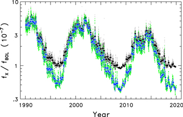
Figure A1. Darker dots represent 81 day (3-rotation) averages of the original FISM2 solar soft X-ray light curve introduced in Paper I; blue dots are for the new version of FISM2 incorporated here in Paper V. Smaller gray and green dots are daily averages for the old and new versions, respectively. New FISM2 has cycle peaks similar to the previous version but significantly lower minima, which changes the cycle MAX/MIN contrast from about 5 to more than 10.
Download figure:
Standard image High-resolution imageThe revision of FISM2 has an impact on the flux–flux correlations pitting X-rays versus various species derived in Papers I (UV) and II (EUV), especially at the low-intensity ends of the scatter diagrams where the new coronal time series reaches to lower fluxes, thereby steepening many of the trends. Figures A2(a), (b), and (c) provide freshly derived flux–flux relations for representative EUV and UV species. The X-rays are always on the y-axis, while the x-axis "X-Line" is noted in the subtitle of each panel. Brackets denote logarithmic values of fL/fBOL. Small orange dots refer to 7 day averages of the X-rays and comparison species; larger darker dots are up-binned averages (accumulated in order of increasing x-axis values: see Paper II for details). Red curves are parabolic fits to the up-binned logarithmic fluxes of the form,

where  for the Y-Line (always X-rays), and similarly x for the X-line (various). The fitted parameters are summarized in Table A1, which is separated into three parts corresponding to the wavelength intervals illustrated in Figure A2 (which, in turn, are related to the different operational periods of the satellite irradiance instruments involved).
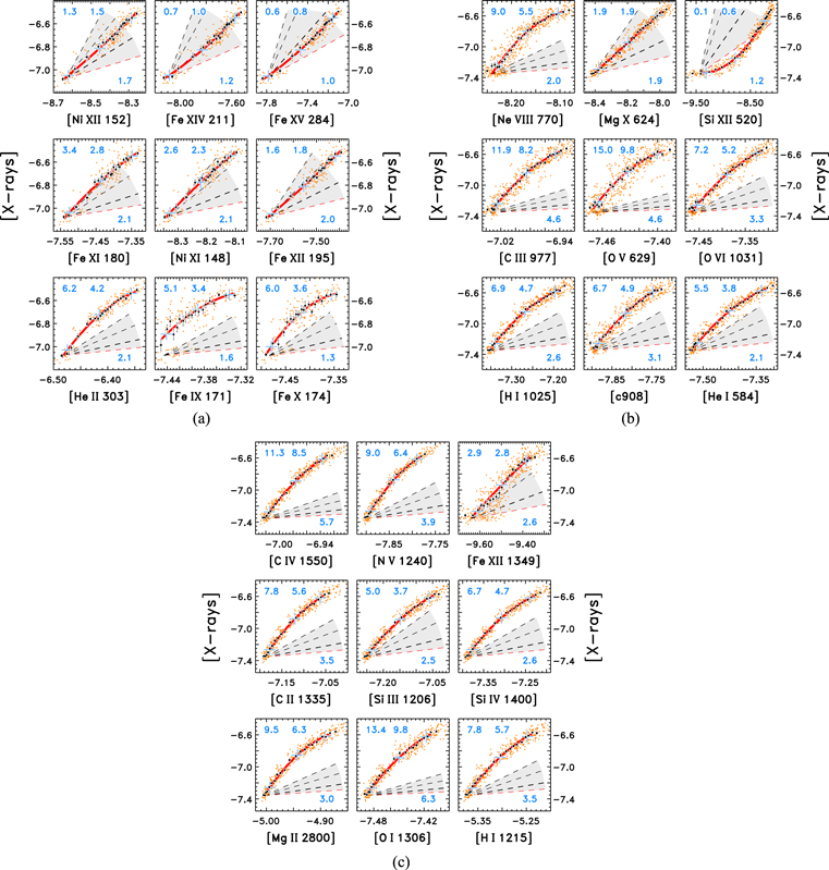
Figure A2. Flux–flux comparisons of solar X-rays (0.2–2 keV) vs. various important EUV and UV species. (a) Short-EUV (140–400 Å); (b) long-EUV (400–1150 Å); (c) UV (1150–3000 Å).
Download figure:
Standard image High-resolution imageTable A1. Solar X-Ray (0.2–2 keV) Power Laws
| X-Line | logT | (xmin, xmax) | x0 | y0 | α15 | α50 | α85 | c1 ± σ1 | c2 ± σ2 | χ2 |
|---|---|---|---|---|---|---|---|---|---|---|
| 1 | 2 | 3 | 4 | 5 | 6 | 7 | 8 | 9 | 10 | 11 |
| Short-EUV | ||||||||||
| Ni xi 148 | 6.2 | (−8.35, −8.10) | −8.22 | −6.78 | 2.6 | 2.3 | 2.1 | 2.34 ± 0.05 | −1.3 ± 0.6 | 1.5 |
| Ni xii 152 | 6.3 | (−8.65, −8.26) | −8.45 | −6.81 | 1.3 | 1.5 | 1.7 | 1.49 ± 0.03 | 0.5 ± 0.2 | 1.3 |
| Fe ix 171 | 5.9 | (−7.45, −7.33) | −7.39 | −6.68 | 5.1 | 3.4 | 1.6 | 3.35 ± 0.05 | −16.9 ± 1.1 | 1.2 |
| Fe x 174 | 6.1 | (−7.49, −7.35) | −7.42 | −6.70 | 6.0 | 3.6 | 1.3 | 3.63 ± 0.11 | −19.2 ± 2.6 | 1.5 |
| Fe xi 180 | 6.2 | (−7.54, −7.33) | −7.44 | −6.76 | 3.4 | 2.8 | 2.1 | 2.76 ± 0.06 | −3.7 ± 1.0 | 1.2 |
| Fe xii 195 | 6.2 | (−7.72, −7.39) | −7.56 | −6.81 | 1.6 | 1.8 | 2.0 | 1.81 ± 0.03 | 0.7 ± 0.4 | 1.5 |
| Fe xiv 211 | 6.3 | (−8.13, −7.53) | −7.83 | −6.83 | 0.7 | 1.0 | 1.2 | 0.96 ± 0.01 | 0.4 ± 0.1 | 1.7 |
| Fe xv 284 | 6.4 | (−7.84, −7.10) | −7.47 | −6.83 | 0.6 | 0.8 | 1.0 | 0.80 ± 0.01 | 0.3 ± 0.1 | 1.2 |
| He ii 303 | 4.9 | (−6.48, −6.35) | −6.42 | −6.72 | 6.2 | 4.2 | 2.1 | 4.16 ± 0.05 | −17.3 ± 0.9 | 2.1 |
| Long-EUV | ||||||||||
| Si xii 520 | 6.9 | (−9.41, −8.15) | −8.78 | −7.15 | 0.1 | 0.6 | 1.2 | 0.63 ± 0.01 | 0.5 ± 0.1 | 1.8 |
| He i 584 | 4.5 | (−7.53, −7.32) | −7.43 | −6.84 | 5.5 | 3.8 | 2.1 | 3.76 ± 0.03 | −9.4 ± 0.6 | 2.6 |
| Mg x 624 | 6.8 | (−8.41, −7.98) | −8.20 | −6.94 | 1.9 | 1.9 | 1.9 | 1.91 ± 0.01 | 0.1 ± 0.1 | 1.5 |
| O v 629 | 5.3 | (−7.47, −7.39) | −7.43 | −6.82 | 15.0 | 9.8 | 4.6 | 9.81 ± 0.21 | −80.9 ± 10.5 | 2.8 |
| Ne viii 770 | 5.8 | (−8.24, −8.09) | −8.17 | −6.80 | 9.0 | 5.5 | 2.0 | 5.49 ± 0.10 | −27.7 ± 2.2 | 1.9 |
| c908 (LyC) | (3.9) | (−7.90, −7.74) | −7.82 | −6.86 | 6.7 | 4.9 | 3.1 | 4.89 ± 0.07 | −13.2 ± 1.4 | 1.2 |
| C iii 977 | 4.8 | (−7.03, −6.94) | −6.99 | −6.84 | 11.9 | 8.2 | 4.6 | 8.22 ± 0.11 | −46.1 ± 4.3 | 1.5 |
| H i 1025 | (4.3) | (−7.35, −7.18) | −7.27 | −6.85 | 6.9 | 4.7 | 2.6 | 4.72 ± 0.04 | −15.1 ± 0.9 | 1.6 |
| O vi 1031 | 5.4 | (−7.47, −7.31) | −7.39 | −6.86 | 7.2 | 5.2 | 3.3 | 5.22 ± 0.06 | −14.9 ± 1.4 | 2.5 |
| UV | ||||||||||
| Si iii 1206 | 4.7 | (−7.25, −7.04) | −7.15 | −6.89 | 5.0 | 3.7 | 2.5 | 3.71 ± 0.03 | −7.1 ± 0.6 | 1.7 |
| H i 1215 | (4.3) | (−5.37, −5.24) | −5.30 | −6.88 | 7.8 | 5.7 | 3.5 | 5.66 ± 0.01 | −19.1 ± 0.1 | 1.3 |
| N v 1240 | 5.2 | (−7.90, −7.78) | −7.84 | −6.87 | 9.0 | 6.4 | 3.9 | 6.43 ± 0.05 | −25.7 ± 1.7 | 1.8 |
| O i 1306 | (3.9) | (−7.49, 7.41) | −7.45 | −6.89 | 13.4 | 9.8 | 6.3 | 9.83 ± 0.10 | −54.9 ± 5.1 | 3.2 |
| C ii 1335 | 4.5 | (−7.19, −7.05) | −7.12 | −6.88 | 7.8 | 5.6 | 3.5 | 5.62 ± 0.05 | −18.5 ± 1.4 | 1.2 |
| Fe xii 1349 | 6.2 | (−9.63, −9.36) | −9.50 | −6.94 | 2.9 | 2.8 | 2.6 | 2.78 ± 0.05 | −0.7 ± 0.7 | 2.5 |
| Si iv 1400 | 4.9 | (−7.39, −7.23) | −7.31 | −6.87 | 6.7 | 4.7 | 2.6 | 4.65 ± 0.04 | −14.7 ± 0.9 | 1.6 |
| C iv 1550 | 5.0 | (−7.02, −6.93) | −6.98 | −6.89 | 11.3 | 8.5 | 5.7 | 8.50 ± 0.07 | −36.7 ± 2.6 | 2.0 |
| Mg ii 2800 | (3.9) | (−5.00, −4.88) | −4.94 | −6.85 | 9.5 | 6.3 | 3.0 | 6.25 ± 0.06 | −31.8 ± 1.8 | 2.7 |
Note. Col. 1 is the X-Line species name. Col. 2 is the temperature (logT in kelvin) of maximum emissivity in CIE from CHIANTI (parenthetical values are estimates for optically thick chromospheric species). Col. 3 gives the range of x (≡log fL/fBOL) for the X-Line. Col. 4 is a reference value, x0, for the X-Line. Col. 5 is the derived y0 (for the X-rays) according to Equation (A1). Cols. 6–8 list slopes, α, at 15%, 50%, and 85% of the x-range, along the curved power laws relating the X-rays to the reference (X-Line) species. Cols. 9 and 10 are the two coefficients of the Equation (A1) fit to the curved power law. Col. 11 is the χ2 of the fit. The single lines O i 1306 Å and C ii 1335 Å are the long wavelength members of the respective multiplets. Blends of two components (1304 Å + 1306 Å; 1334 Å + 1335 Å) in the original low-resolution solar scans were scaled to the single-component values according to relative line strengths deduced from high-resolution spectra.
Download table as: ASCIITypeset image
In each of the panels of Figure A2, the X-line species are arrayed from left to right, and bottom to top, in rough order of increasing formation temperature. In the panels, a shaded fan of dashed straight lines represents reference power laws: α = 0.5 (red); 1 (2nd from bottom, darker); 2 (next higher); and 3 (highest). Blue pluses mark points along the curved power laws, at 15% (left) of the species x range ( to
to  ), 50% (middle), and 85% (right). Aligned blue values at the top and bottom of each panel refer to the slopes of the curves at the three reference points. These slope values are also listed in Table A1.
Note that many of the flux–flux relations begin steeply, at low x, but then flatten at higher x. The apparent correlations would be a good target for modelers to explain, but also have potential utility in scaling inaccessible stellar EUV species from more accessible proxies, such as X-rays or Mg ii.
Appendix B: STIS Wavelength Corrections
An important side story of the present HST/STIS study was a scheme to correct the high-dispersion stellar echellegrams for subtle wavelength errors devolving from the inability of the low-order polynomial dispersion model embedded in the CALSTIS pipeline to track apparent higher order spatial geometrical distortions in the MAMA camera images (see, e.g., Ayres 2010). The ASTRAL Project, mentioned earlier, developed high-order 2D polynomial corrections, containing up to several dozen terms, to account for these subtle but widespread distortions. The approach, albeit complex, worked well at the time and still is the gold standard. However, there is a simpler way that is based on the fact that the major deviations in the 2D wavelength residuals typically were cross-dispersion, from the bottom of the echelle pattern to the top (dominant wavelength axis), rather than from one side of an echelle order to the other. Thus, a simple 1D polynomial of modest order in the wavelength direction can provide most of the desired correction. The full implementation for all 44 supported STIS echelle settings will be described elsewhere (Ayres 2022), but a preview is provided here for the four FUV (1 M, 3 H) and four NUV (all H) settings that contributed to the long-term synoptic programs on α Cen AB and Procyon.
Figures B1(a) and (b) illustrate wavelength displacements for those specific STIS settings. The offsets were measured in co-added calibration lamp spectra, processed through the standard CALSTIS pipeline as if science images. Each panel depicts the displacements relative to the laboratory values and expressed in equivalent velocities, as a function of wavelength across the grasp of the particular setting. The y-axis scales correspond roughly to ±1 resel. The smooth dashed curve is a polynomial fit of order 3, or higher in some cases (the bivariate dispersion model in CALSTIS is second order). Yellow circled points are outliers excluded from the fit. The derived long-range wavelength corrections are highly significant, yet the amplitudes typically are only a fraction of a resel (well within the original engineering specifications). Nevertheless, the true wavelength precision of STIS challenges the quality delivered by the current CALSTIS dispersion model.
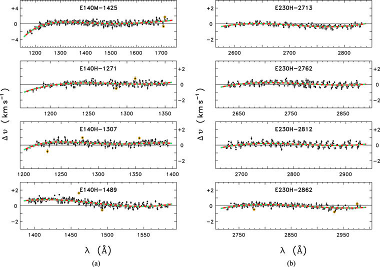
Figure B1. Examples of the wavelength corrections for STIS settings used in the current study. Each panel depicts wavelength offsets, λobs − λLAB, expressed as equivalent velocities, as a function of wavelength. The y-axis scales correspond roughly to ±1 resel. Smooth dashed curves are polynomials of order 3, or higher in some cases. Yellow circled points were excluded as outliers. (a) FUV workhorse E140M-1425 and three E140H settings. (b) Four adjacent, overlapping E230H settings that all capture the key Mg ii 2796 Å + 2803 Å chromospheric resonance doublet.
Download figure:
Standard image High-resolution imageIn only two of the eight cases were polynomials of degree greater than n = 3 required: E140M-1425 (n = 5) and E140H-1307 (n = 4). This is a dramatic improvement in simplicity compared to the complex 2D models in the ASTRAL protocols (see also Ayres 2010). Empirical velocity residuals of corrected wavecals now are near the limits imposed by measurement errors and knowledge of the laboratory wavelengths. Indeed, the corrections for the NUV-H settings illustrated here were relatively minor, only fractions of a resel, although still significant and systematic. The derived polynomial corrections were applied to the stellar x1d files to suppress the subtle but systematic wavelength distortions that are otherwise present, which allowed fairer velocity comparisons to be made across the full grasp of a given echelle setting.
Appendix C: Additional Examples of STIS Spectral Fits: α Cen B and Procyon, Medium and High Resolution
This appendix provides additional examples of spectral fits, specifically for epoch-average α Cen B (Figure C1(a) (M resolution) and C1(b) (H)) and Procyon (Figure C2(a) (M) and C2(b) (H)). The FUV-H tracings display sharper interstellar absorptions in the H i, O i, and C ii resonance lines but have higher noise levels, especially at the two faint Fe xii coronal forbidden lines. In addition, the normalization of the c1506 band can change because the local maximum is dictated by a narrow emission line (right-hand side), which is more resolved and has a higher peak in FUV-H. The NUV panels are the same in the M and H figures for each star because that region was observed exclusively in H resolution. Note the curved "continuum" at Fe xii 1241 Å in the Procyon spectra. The coronal forbidden line sits on the blue wing of N v 1242 Å, which is broader in the subgiant and thus more strongly influences the background at 1241 Å.
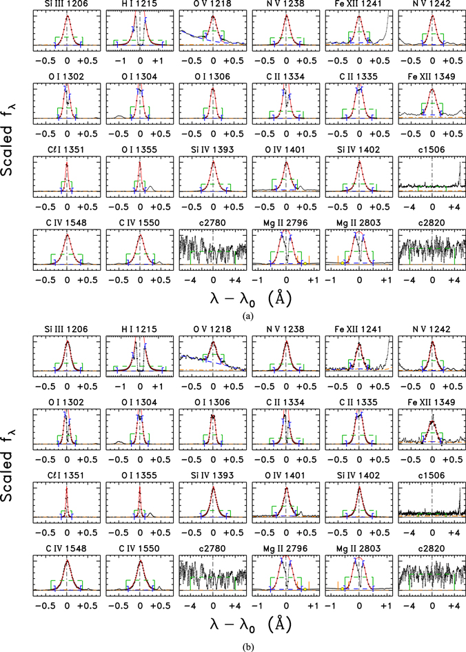
Figure C1. Examples of spectral fits for α Cen B. See the caption for Figure 5 for further details. (a) Medium-resolution epoch-average spectrum. (b) High-resolution epoch-average spectrum.
Download figure:
Standard image High-resolution image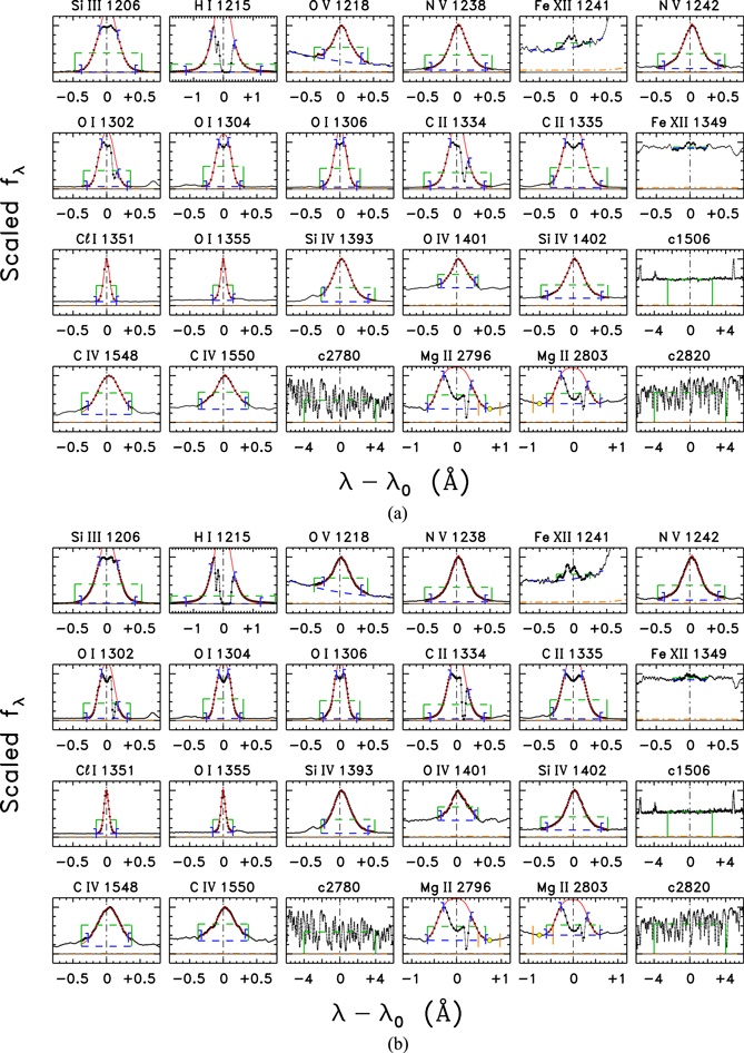
Figure C2. Examples of spectral fits for Procyon. See the caption of Figure 5 for further details. (a) Medium-resolution epoch-average spectrum. (b) High-resolution epoch-average spectrum.
Download figure:
Standard image High-resolution image
Table C1, similar to previous Table 7, compares the line shape measurements of the FUV-M and FUV-H spectra of α Cen B and Procyon.
Table C1. Epoch-average α Cen B and Procyon: FUV M vs. H
| Species | Star | Res | υ ± συ | FWHM ± σFW | a ± σa | fL/fBOL | fC/fBOL |
|---|---|---|---|---|---|---|---|
| (km s−1) | (10−7) | (10−7 Å−1) | |||||
| 1 | 2 | 3 | 4 | 5 | 6 | 7 | 8 |
| Si iii 1206 | B | M | +4.7 ± 0.1 | 45.8 ± 0.2 | 1.71 ± 0.01 | 1.08 | 0.00 |
| B | H | +4.5 ± 0.1 | 41.4 ± 0.2 | 1.60 ± 0.01 | 1.18 | 0.0285 | |
| P | M | +5.0 ± 0.1 | 77.2 ± 1.2 | 1.71 ± 0.03 | 2.42 | 0.00 | |
| P | H | +3.8 ± 0.1 | 74.8 ± 0.5 | 1.68 ± 0.01 | 2.55 | 0.078 | |
| H i 1215 | B | M | −0.2 ± 0.1 | 57.7 ± 0.2 | 1.00 ± 0.00 | 51 | 0.085 |
| B | H | +0.1 ± 0.1 | 58.2 ± 0.2 | 1.00 ± 0.00 | 54 | 0.00 | |
| P | M | −5.6 ± 0.1 | 79.1 ± 0.5 | 1.00 ± 0.00 | 26.0 | 0.159 | |
| P | H | −5.1 ± 0.1 | 80.5 ± 0.2 | 1.00 ± 0.00 | 27.8 | 0.031 | |
| O v 1218 | B | M | +2.6 ± 0.2 | 46.3 ± 0.7 | 1.74 ± 0.07 | 0.175 | 0.131 |
| B | H | +3.4 ± 0.2 | 43.5 ± 0.8 | 1.63 ± 0.08 | 0.179 | 0.37 | |
| P | M | +6.7 ± 0.3 | 68.8 ± 1.0 | 1.48 ± 0.05 | 0.35 | 0.33 | |
| P | H | +5.6 ± 0.1 | 71.0 ± 0.4 | 1.51 ± 0.02 | 0.40 | 0.39 | |
| N v 1238 | B | M | +3.5 ± 0.1 | 42.3 ± 0.3 | 1.53 ± 0.02 | 0.219 | 0.0101 |
| B | H | +4.1 ± 0.1 | 39.1 ± 0.4 | 1.48 ± 0.02 | 0.228 | 0.0098 | |
| P | M | +7.0 ± 0.1 | 71.2 ± 0.5 | 1.51 ± 0.02 | 0.49 | 0.066 | |
| P | H | +7.5 ± 0.1 | 67.5 ± 0.2 | 1.45 ± 0.01 | 0.54 | 0.070 | |
| Fe xii 1241 | B | M | −0.0 ± 0.3 | 44.5 ± 0.8 | 1.84 ± 0.08 | 0.0258 | 0.0119 |
| B | H | +1.0 ± 0.4 | 39.5 ± 1.2 | 1.75 ± 0.12 | 0.0274 | 0.0130 | |
| P | M | ⋯ | ⋯ | ⋯ | 0.0068 | 0.077 | |
| P | H | ⋯ | ⋯ | ⋯ | 0.0080 | 0.084 | |
| N v 1242 | B | M | +2.8 ± 0.1 | 43.1 ± 0.3 | 1.63 ± 0.02 | 0.106 | 0.0103 |
| B | H | +4.0 ± 0.2 | 38.6 ± 0.6 | 1.53 ± 0.04 | 0.107 | 0.0107 | |
| P | M | +6.9 ± 0.2 | 69.6 ± 0.6 | 1.41 ± 0.02 | 0.260 | 0.063 | |
| P | H | +7.2 ± 0.1 | 68.3 ± 0.3 | 1.38 ± 0.01 | 0.283 | 0.066 | |
| O i 1302 | B | M | +0.1 ± 0.1 | 35.0 ± 0.2 | 1.97 ± 0.02 | 0.45 | 0.0087 |
| B | H | +0.2 ± 0.1 | 29.2 ± 0.4 | 1.90 ± 0.03 | 0.47 | 0.0051 | |
| P | M | +0.7 ± 0.1 | 58.9 ± 0.5 | 2.31 ± 0.04 | 0.63 | 0.133 | |
| P | H | +0.8 ± 0.1 | 58.7 ± 0.2 | 2.47 ± 0.02 | 0.69 | 0.134 | |
| O i 1304 | B | M | −0.4 ± 0.1 | 30.4 ± 0.4 | 1.83 ± 0.03 | 0.55 | 0.0094 |
| B | H | +0.3 ± 0.1 | 27.0 ± 0.4 | 1.84 ± 0.03 | 0.57 | 0.0087 | |
| P | M | +0.8 ± 0.1 | 57.3 ± 0.3 | 2.65 ± 0.04 | 0.75 | 0.147 | |
| P | H | +1.2 ± 0.1 | 54.6 ± 0.1 | 2.61 ± 0.02 | 0.83 | 0.136 | |
| O i 1306 | B | M | −0.5 ± 0.1 | 32.9 ± 0.1 | 2.17 ± 0.01 | 0.58 | 0.0052 |
| B | H | +0.2 ± 0.1 | 31.4 ± 0.1 | 2.50 ± 0.02 | 0.62 | 0.0011 | |
| P | M | +0.8 ± 0.1 | 45.5 ± 0.3 | 1.97 ± 0.02 | 0.83 | 0.131 | |
| P | H | +0.8 ± 0.1 | 45.1 ± 0.1 | 2.06 ± 0.01 | 0.89 | 0.135 | |
| C ii 1334 | B | M | +1.3 ± 0.1 | 24.0 ± 0.4 | 1.25 ± 0.02 | 0.77 | 0.0065 |
| B | H | +1.3 ± 0.1 | 17.6 ± 0.6 | 1.10 ± 0.02 | 0.82 | 0.0081 | |
| P | M | +2.6 ± 0.1 | 56.0 ± 0.6 | 1.57 ± 0.02 | 1.72 | 0.176 | |
| P | H | +2.2 ± 0.1 | 54.7 ± 0.3 | 1.58 ± 0.01 | 1.84 | 0.197 | |
| C ii 1335 | B | M | +0.8 ± 0.1 | 45.1 ± 0.1 | 1.88 ± 0.01 | 1.37 | 0.0059 |
| B | H | +0.3 ± 0.1 | 40.8 ± 0.3 | 1.81 ± 0.02 | 1.45 | 0.0109 | |
| P | M | +2.2 ± 0.1 | 76.1 ± 0.5 | 2.02 ± 0.02 | 2.40 | 0.183 | |
| P | H | +1.7 ± 0.1 | 72.7 ± 0.3 | 1.96 ± 0.01 | 2.53 | 0.205 | |
| Fe xii 1349 | B | M | +0.1 ± 0.4 | 46.9 ± 1.1 | 2.05 ± 0.15 | 0.0114 | 0.0066 |
| B | H | +0.5 ± 0.6 | 45.6 ± 1.7 | 2.06 ± 0.25 | 0.0121 | 0.0067 | |
| P | M | ⋯ | ⋯ | ⋯ | 0.0034 | 0.204 | |
| P | H | ⋯ | ⋯ | ⋯ | 0.0048 | 0.214 | |
| Cl i 1351 | B | M | −0.2 ± 0.1 | 15.6 ± 0.1 | 1.73 ± 0.03 | 0.054 | 0.0067 |
| B | H | −0.3 ± 0.1 | 9.4 ± 0.1 | 1.54 ± 0.03 | 0.058 | 0.0050 | |
| P | M | −0.1 ± 0.1 | 22.1 ± 0.1 | 1.82 ± 0.02 | 0.240 | 0.208 | |
| P | H | −0.3 ± 0.1 | 18.5 ± 0.1 | 1.79 ± 0.01 | 0.249 | 0.221 | |
| O i 1355 | B | M | −0.4 ± 0.1 | 15.5 ± 0.1 | 1.61 ± 0.02 | 0.084 | 0.0079 |
| B | H | +0.1 ± 0.1 | 9.7 ± 0.1 | 1.38 ± 0.02 | 0.087 | 0.0072 | |
| P | M | −0.0 ± 0.1 | 20.0 ± 0.2 | 1.54 ± 0.02 | 0.176 | 0.215 | |
| P | H | +0.2 ± 0.1 | 15.9 ± 0.1 | 1.44 ± 0.01 | 0.185 | 0.236 | |
| Si iv 1393 | B | M | +2.7 ± 0.1 | 35.2 ± 0.1 | 1.37 ± 0.01 | 0.61 | 0.0107 |
| B | H | +3.4 ± 0.1 | 31.4 ± 0.2 | 1.30 ± 0.01 | 0.69 | 0.0136 | |
| P | M | +5.1 ± 0.1 | 65.3 ± 0.2 | 1.55 ± 0.01 | 1.15 | 0.32 | |
| P | H | +5.6 ± 0.1 | 63.5 ± 0.1 | 1.52 ± 0.01 | 1.36 | 0.37 | |
| O iv 1401 | B | M | +3.2 ± 0.2 | 38.6 ± 0.5 | 1.60 ± 0.04 | 0.049 | 0.0132 |
| B | H | +3.4 ± 0.2 | 33.1 ± 0.8 | 1.40 ± 0.05 | 0.057 | 0.0136 | |
| P | M | +7.2 ± 0.3 | 57.5 ± 0.8 | 1.53 ± 0.06 | 0.164 | 0.34 | |
| P | H | +7.0 ± 0.2 | 58.3 ± 0.6 | 1.55 ± 0.05 | 0.196 | 0.38 | |
| Si iv 1402 | B | M | +3.0 ± 0.1 | 34.8 ± 0.2 | 1.37 ± 0.01 | 0.32 | 0.0120 |
| B | H | +3.2 ± 0.1 | 30.6 ± 0.3 | 1.30 ± 0.01 | 0.36 | 0.0137 | |
| P | M | +4.4 ± 0.1 | 61.3 ± 0.4 | 1.44 ± 0.02 | 0.63 | 0.35 | |
| P | H | +4.8 ± 0.1 | 59.5 ± 0.3 | 1.40 ± 0.01 | 0.74 | 0.39 | |
| c1506 | B | M | ⋯ | ⋯ | ⋯ | 0.136 | ⋯ |
| B | H | ⋯ | ⋯ | ⋯ | 0.155 | ⋯ | |
| P | M | ⋯ | ⋯ | ⋯ | 4.1 | ⋯ | |
| P | H | ⋯ | ⋯ | ⋯ | 4.7 | ⋯ | |
| C iv 1548 | B | M | +2.9 ± 0.1 | 41.1 ± 0.1 | 1.47 ± 0.01 | 1.25 | 0.0192 |
| B | H | +3.3 ± 0.1 | 39.6 ± 0.2 | 1.49 ± 0.01 | 1.31 | 0.0260 | |
| P | M | +6.7 ± 0.1 | 75.9 ± 0.2 | 1.93 ± 0.02 | 2.78 | 1.36 | |
| P | H | +6.9 ± 0.1 | 75.2 ± 0.2 | 1.88 ± 0.02 | 3.1 | 1.44 | |
| C iv 1550 | B | M | +2.9 ± 0.1 | 41.6 ± 0.2 | 1.56 ± 0.01 | 0.62 | 0.0194 |
| B | H | +4.1 ± 0.1 | 38.2 ± 0.3 | 1.47 ± 0.02 | 0.67 | 0.0208 | |
| P | M | +4.6 ± 0.1 | 63.8 ± 0.4 | 1.37 ± 0.02 | 1.41 | 1.45 | |
| P | H | +6.1 ± 0.1 | 62.7 ± 0.3 | 1.38 ± 0.02 | 1.55 | 1.63 | |
Note. Col. 1 is the species name. Col. 2 indicates the star (B = α Cen B; P = Procyon) for the epoch-average FUV spectrum. Col. 3 is the resolution mode: M for medium; H for high. Col. 4 is the velocity shift of the species relative to narrow, low-excitation lines. Col. 5 is the derived line width expressed in velocity units. Col. 6 is the fitted pseudo-Gaussian exponent. Col. 7 is the measured normalized integrated line flux. Col. 8 is the background continuum level at line center, in normalized flux density units.
Footnotes
- 1
- 2
- 3
- 4
The STIS slits are specified as height × width, both in arcseconds.
- 5
- 6
The background emission levels, contributed typically by photoionization continua that vary smoothly with wavelength, were estimated through a hierarchical filtering of the flux densities in a large interval surrounding the target line of interest. See Paper I for details.
- 7
The 1241 Å Fe xii component could not be measured in the solar irradiance scans described in Paper I, but its weaker sibling at 1349 Å was free-enough of extraneous blends to successfully be captured. However, the STIS echelle spectra of AB and Procyon adequately separate 1241 Å from adjacent N v 1242 Å, so both Fe xii components are available for the stars. To be compatible with the solar measurements of the 1349 Å component alone, the pair of stellar Fe xii lines were combined into a single "1349 Å" flux, based on ratios of the components in the high-S/N epoch-average FUV-M spectrum of α Cen B. Thus, future references to Fe xii 1349 Å for the STIS stars are to be understood as the scaled sum of the two components.
- 8
1334 Å was a better choice than 1335 Å for the solar Doppler measurements, owing to lower optical thickness. However, in the stars, 1335 Å is preferred because the 1334 Å resonance transition is strongly affected by interstellar absorption.