


Abstract
Given the infrequency of extreme geomagnetic storms, it is significant to note the concentration of three extreme geomagnetic storms in 1941, whose intensities ranked fourth, twelfth, and fifth within the aa index between 1868–2010. Among them, the geomagnetic storm on 1941 March 1 was so intense that three of the four Dst station magnetograms went off scale. Herein, we reconstruct its time series and measure the storm intensity with an alternative Dst estimate (Dst*). The source solar eruption at 09:29–09:38 GMT on February 28 was located at RGO AR 13814 and its significant intensity is confirmed by large magnetic crochets of ∣35∣ nT measured at Abinger. This solar eruption most likely released a fast interplanetary coronal mass ejection with estimated speed 2260 km s−1. After its impact at 03:57–03:59 GMT on March 1, an extreme magnetic storm was recorded worldwide. Comparative analyses on the contemporary magnetograms show the storm peak intensity of minimum Dst* ≤ −464 nT at 16 GMT, comparable to the most and the second most extreme magnetic storms within the standard Dst index since 1957. This storm triggered significant low-latitude aurorae in the East Asian sector and their equatorward boundary has been reconstructed as 38 5 in invariant latitude. This result agrees with British magnetograms, which indicate an auroral oval moving above Abinger at 530 in magnetic latitude. The storm amplitude was even more enhanced in equatorial stations and consequently casts caveats on their usage for measurements of the storm intensity in Dst estimates.
Export citation and abstract BibTeX RIS
1. Introduction
Solar eruptions occasionally direct interplanetary coronal mass ejections (ICMEs) toward the Earth. When they have sufficient speed, mass, and southward interplanetary magnetic field (IMF), such geoeffective ICMEs cause serious geomagnetic storms and variations in the terrestrial magnetic field (Gonzalez et al. 1994; Daglis et al. 1999). Intensities of the subsequent geomagnetic storms have been usually measured with the negative excursion in the disturbance storm time (Dst) index since the International Geophysical Year (IGY: 1957–1958) as a representative of the ring current intensity. The Dst index is based on the average of the four midlatitude magnetic disturbances at four reference stations (e.g., Sugiura 1964; Sugiura & Kamei 1999; WDC for Geomagnetism at Kyoto et al. 2015). Partially due to their geoeffectiveness, such solar eruptions have been subjected to astronomical interests from the early phase of the modern astrophysical studies (e.g., Carrington 1859; Hale 1931; Cliver 2006; Gopalswamy 2016; Tsurutani et al. 2020).
Within this chronological coverage, it was the 1989 March storm that recorded the most extreme intensity (minimum Dst = −589 nT; WDC for Geomagnetism at Kyoto et al. 2015). This storm dramatically extended the auroral oval equatorward and had serious economic impacts on modern society with its space weather hazards (e.g., Allen et al. 1989; Cid et al. 2014; Pulkkinen et al. 2017; Riley et al. 2018; Boteler 2019). This case shows that such extreme geomagnetic storms are not only of academic interest, but also of societal interest due to our increasing reliance on modern technological infrastructure (e.g., Pulkkinen et al. 2017; Riley et al. 2018). Such extreme storms have been studied in terms of their chronological distributions (Kilpua et al. 2015; Lefèvre et al. 2016) and revealed apparent correlations between the storm intensity and equatorward boundary of the auroral oval (Yokoyama et al. 1998).
Statistical analyses of such extreme storms are challenging as they are rare (Yermolaev et al. 2013) and only five storms went below the threshold of Dst = −400 nT within the coverage of the Dst index routinely derived by WDC Kyoto (Riley et al. 2018; Meng et al. 2019). Among them, only the 1989 March storm developed beyond the threshold of Dst = −500 nT and has been considered as a superstorm (e.g., Boteler 2019). Furthermore, reconstructions of historical superstorms have shown that geomagnetic superstorms such as the events occurring in 1859 September, 1872 February, and 1921 May set further benchmarks both in terms of storm intensities (minimum Dst ≤ −800 nT) and equatorward boundaries of the auroral oval (e.g., Tsurutani et al. 2003; Silverman & Cliver 2001; Green & Boardsen 2006; Siscoe et al. 2006; Gonzalez et al. 2011; Cliver & Dietrich 2013; Lakhina & Tsurutani 2017; Hayakawa et al. 2018a, 2018b, 2019a, 2020c; Love et al. 2019b; Blake et al. 2020). Their impacts on modern technological infrastructure on the ground and in space are estimated to be even more catastrophic than their historical impacts (Daglis 2001; Baker et al. 2008; Cannon et al. 2013; Hapgood 2017; Riley et al. 2018; Oliveira et al. 2020).
Despite existing efforts on the extension of the Dst index (e.g., Mursula et al. 2008), it is challenging to quantitatively measure the intensity of geomagnetic superstorms before the IGY, as their significant intensity frequently makes contemporary magnetograms run off scale (Riley 2017, p. 118) and geographical coverage of historical magnetograms was much scarcer in the past. As such, Dst estimates (Dst*) for several superstorms have been reconstructed with alternative magnetograms in midlatitude, with reasonable longitudinal separation, and quasi-completeness in the hourly resolution. These case studies have been conducted on four geomagnetic superstorms in 1903 October/November (minimum Dst* ≈ −513 nT; Hayakawa et al. 2020b), 1909 September (minimum Dst* ≈ −595 nT; Hayakawa et al. 2019b; Love et al. 2019a), 1921 May (minimum Dst* ≈ −907 ± 132 nT; Love et al. 2019b), and 1946 March (minimum Dst* ≤ −512 nT; Hayakawa et al. 2020a).
However, historical magnetograms show that these storms are only a small sample of extreme geomagnetic storms in history. Among them, the geomagnetic conditions in 1941 were especially notable, hosting at least three geomagnetic storms in March, July, and September, which ranked fourth, twelfth, and fifth within the aa index in 1868–2010, respectively (Lefèvre et al. 2016). Colorful auroral episodes for the 1941 September storm have been introduced in Love & Coïsson (2016), whereas little is known for the other two. On the other hand, the 1941 March storm had equally or even more extreme episodes, with magnetograms at three of four Dst stations going off scale. In fact, this storm had the third largest ΔH deviation measured at the Greenwich-Abinger observatories (1650 nT to 1710 nT) within the 112 great storms during 1874–1954 (Jones 1955, p. 79; see also Newton 1941) and was ranked the fourth most intense within the aa index during 1868–2010 (Lefèvre et al. 2016). Shifting down to the midlatitudes, this storm ranked in the seventh largest (>560 nT) within the storms recorded at Kakioka ΔH between 1924 and 2020,12 despite its incomplete measurement. Therefore, in this article, we analyze the time series of this extreme space/geomagnetic storm on 1941 March 1 with its source flare on 1941 February 28 from its source solar eruption to its terrestrial impact. In addition, we measure its intensity in Dst* based on alternative magnetograms and examine the equatorial boundary of the auroral oval.
2. Solar Eruption
In the declining phase of Solar Cycle 17 after its maximum in 1937 April (Table 1 of Hathaway 2015; Figure 2 of Clette & Lefèvre 2016), the solar surface in late February to early March of 1941 was moderately eruptive but not as much as in April–September. Of the 27 solar flares recorded in the Hα observations in 1941 February–March, 7 flares were observed over RGO AR 13814 (Brunner 1942). Those flares were mostly categorized as 1 (Hα flare area = 100–250 msh) to 2 (Hα flare area = 250– 600 msh) in their Hα flare area, whereas one on 1941 March 3 achieved importance of 3 (Hα flare area = 600–1200 msh) (Brunner 1942; see also Švestka 1976, p. 14).
Upon contemporary observations, Newton (1941, p. 84) apparently associated our great storm with "a fairly large sunspot not far from the central meridian." As shown in Figure 1, Newton (1941) most likely indicated RGO AR 13814 with this description. As well as the chromospheric eruptions, Newton (1941) listed three notable ionospheric disturbances with "wireless fade-outs" as footprints of solar flares at 15:45–16:10 GMT on February 27, and 09:30–10:30 GMT and 15:27–15:40 GMT on February 28. Among them, Newton (1941, p. 84) considered the second wireless fade-out as the source eruption and clarified the sky over Greenwich overcast. The third fade-out coincides chronologically with "a very small sudden commencement disturbance" at 15:26 GMT on February 28 reported at Hermanus (Ogg 1941, p. 372), which may actually be an SFE misinterpreted as an SSC. This sunspot developed to 650 millionth solar hemisphere immediately after its central meridian passage on 1941 February 27.3 (Newton 1941, p. 85).
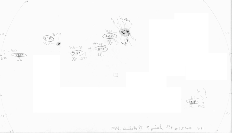
Figure 1. Sunspot drawing at Mt. Wilson on 1941 February 27 with its side corrected, as viewed in the sky. The MWO AR 7132 corresponds to RGO AR 13814 (courtesy of the Mt. Wilson Observatory; see also Pevtsov et al. 2019).
Download figure:
Standard image High-resolution imageContemporary magnetograms confirm his discussions with magnetic crochets (see McIntosh 1951), as footprints of intense X-ray radiation of solar flares (see Curto et al. 2016; Curto 2020). Figure 2 shows digitized magnetograms at Abinger, Eskdalemuir, and Lerwick on 1941 February 28–March 1. We have digitized their scans hosted by BGS13 based on the scale units shown in Hartnell (1922, p. 2) and the min–max scale values given in the observatory yearbooks (AMMO 1958, p. 21, 109; Jones 1954, p. D21). Our digitizations have located magnetic crochets around 09:29–09:38 GMT on February 28 with notable amplitudes: ≈∣13∣ nT at Lerwick, ≈∣20∣ nT, at Eskdalemuir, and ≈∣35∣ nT at Abinger, respectively (see also McIntosh 1951; Jones 1955, p. 81).

Figure 2. Magnetic disturbances at Lerwick, Eskdalemuir, Abinger, and Hermanus spanning from 1941 February 28 to March 1 digitized from their original magnetograms at BGS and trace copy of Ogg (1941). These magnetograms show magnetic crochets at 09:29–09:38 GMT and the SSCs at 03:57–03:59 GMT.
Download figure:
Standard image High-resolution imageInterestingly, significant polar cap absorption was reported at Tikhaya Bay (N80°19', E052°47') for 4 days from somewhere between 22 GMT on February 26 and 06 GMT on February 27 and caused blackouts for 99 hr (Besprozvannaya 1962, p. 147; see also Cliver et al. 1990, p. 17109). Such polar cap absorptions indicate a presence of solar proton events (e.g., Shea & Smart 2012), as shown from their known pairs with the intense solar proton events (Besprozvannaya 1962; McCracken 2007; Usoskin et al. 2020). While only one minor flare was reported in this onset interval (0:36 GMT on February 27 at Mt. Wilson; Brunner 1942, p. 80), this implies some of the flares in this sequence from RGO AR 13814 probably caused notable solar proton events. This implies that the source flare around 09:29–09:38 GMT on February 28 also possibly caused a solar proton event.
3. Interplanetary Coronal Mass Ejection
These magnetic crochets were followed by sudden storm commencements (SSCs) at ≈03:57–03:59 on March 1, as summarized in Table 1. Among them, Hermanus reported two SSCs at 03:58 (ΔH = 42 nT) and 05:19 (ΔH = 48 nT), which probably indicates arrivals of at least two consecutive ICMEs. The time lag between the magnetic crochet and the SSCs shows the transit time of the ICME as 18.4 hr and imply the average speed of this ICME as 2260 km s−1.
Table 1. Recorded Amplitudes of SSC and Geomagnetic Storms (ΔH) at Each Observatory
| Observatory | Lat. | Long. | Mlat. | Mlon. | SSC | H-range | References |
|---|---|---|---|---|---|---|---|
| Hermanus* | S34°25' | E019°13' | −33.2 | 80.0 | 42&48 | 614 | Ogg (1941) |
| Watheroo* | S30°19' | E115°52' | −41.8 | −174.9 | 19 | 658 | Parkinson (1941) |
| Tucson* | N32°15' | W110°50' | 40.4 | −48.4 | 74 | >550 | White (1941) |
| Apia* | S13°48' | W171°45' | −16.2 | −100.2 | WDC Kyoto | ||
| Kakioka | N36°14' | E140°11' | 26.0 | −154.5 | 31 | >560 | KED |
| Alibag | N18°38' | E072°52' | 9.5 | 143.2 | 42 | >785 | Rangaswami (1941) |
| Huancayo | S12°02' | W076°20' | −0.6 | −7.6 | 80 | 1180 | Ledig (1941) |
| Abinger | N50°11' | E000°23' | 53.0 | 83.1 | 50 | 1650 | Figure 2 |
| Eskdalemuir | N55°19' | W003°12' | 58.6 | 82.5 | 55 | 1320 | Figure 2 |
| Lerwick | N60°08' | W001°11' | 62.6 | 88.2 | 40 | 1180 | Figure 2 |
Note. Magnetic coordinates (mlat. and mlon.) are computed with the IGRF-12 model (Thébault et al. 2015). The stations with asterisks (*) are the reference stations in our estimate. The observational data at Apia are acquired only with its hourly value from the WDC Kyoto (WDC for geomagnetism at Kyoto) and do not show the SSC amplitude and the H-variation in the spot value.
Download table as: ASCIITypeset image
Siscoe et al. (1968) and Burton et al. (1975) provide the following empirical formula for dynamic pressure computations as a function of geomagnetic field variations:

At the instance of maximum compression, Dst* shows the SSC amplitude ΔB ≈ 35 nT, and Equation (1) yields ΔPd ≈ 4.9 nPa. This ram pressure is almost 8 times larger than the ram pressure during quiet solar wind conditions, namely ≈0.75 nPa for solar wind speed of 300 km s−1 and solar wind density of 5 cm−3. In addition, by assuming equilibrium conditions during the interactions of the magnetosphere with the solar wind, the resulting inward magnetopause position is given by Baumjohann & Treumann (2009):

where B0 is the contemporary dipole magnetic field at the Earth's surface at L = 1, μ0 is the vacuum permeability, and K is an arbitrary factor. According to the IGRF model for the epoch of 1940 (Thébault et al. 2015), the spherical harmonic coefficients  ,
,  , and
, and  are −30,654 nT, −2292 nT, and 5821 nT, respectively, which yield B0 of 31,286 nT. Assuming that K = 2 and that Pd = 5.65 nPa (=0.75 + 4.9 nPa), we compute Xmp ≈ 7.2 RE. Comparing this result with the magnetopause standoff position during nominal solar wind conditions (≈10.1RE for Pd = 0.75 nPa), one concludes that the magnetopause moved ≈3RE inwards. However, the magnetopause did not surpass the threshold of geosynchronous orbit (≈6.6 RE), which could expose satellites to the hostile solar wind environment (e.g., Baker et al. 2018). The most inward observed magnetopause motion, ≈5.24 RE from the Earth's center (Hoffman et al. 1975) occurred as a result of the impact of the fastest CME to hit Earth ever recorded, with speed of 2850 km s−1 (Vaisberg & Zastenker 1976; Cliver et al. 1990). Therefore, these results show that the impact of the probable CME in 1941 March had moderate compression of the Earth's magnetosphere.
4. Magnetic Disturbance
After the ICME arrival at 03:57 GMT, the intense magnetic storm developed so rapidly that a number of the ground-based magnetograms went off scale at that time. This makes the intensity estimate for this storm rather challenging. While the Dst index has been used to evaluate storm intensity as a quantitative measurement for the ring current development, the 1941 March storm occurred far before its introduction. The standard Dst index has been measured with an average of the four stations (Kakioka, Honolulu, San Juan, and Hermanus) with weighting of their magnetic latitude (Sugiura 1964; WDC for Geomagnetism at Kyoto et al. 2015). However, the 1941 March storm was only incompletely recorded at three of these standard stations, due to the data gaps during 14–16 and 18 GMT at Kakioka, 16–17 GMT at Honolulu, and 14–22 GMT at San Juan14 . These data gaps affect any attempts to extend the Dst index upon this storm with the use of existing Dst reference stations (see Riley et al. 2018; Karinen & Mursula 2005; Mursula et al. 2008).
As such, we need to substitute these three stations with three mid- to low-latitude magnetograms in similar magnetic longitudes without significant data gaps to estimate the Dst equivalent measurement of the storm intensity. Three magnetograms at Watheroo (WAT), Apia (API), and Tucson (TUC) satisfy this requirement and are used to replace the incomplete data from Kakioka, Honolulu, and San Juan, respectively. We have derived their hourly data from the WDC for geomagnetism at Kyoto. Following the procedure of the standard Dst calculations, we have first derived the hourly disturbance at each station (Di (t)), subtracting the baseline (Bi) and solar quiet field variations (Sqi (t)). We then averaged the hourly disturbance at each station with weighting of their contemporary magnetic latitude (λi) (Sugiura 1964; WDC for Geomagnetism at Kyoto et al. 2015). These calculations are summarized by the following two equations.


In our analyses, the baseline (Bi) has been approximated with the observatory annual means for each station, provided in the WDC for geomagnetism at Edinburgh.15 The solar quiet field variation (Sqi (t)) has been approximated with the five quietest days in the previous month of this storm (1941 February 27, 12, 19, 18, and 1), which have been selected on the basis of the revised daily aa index provided in Lockwood et al. (2018a, 2018b). The magnetic latitude of each station in 1941 has been computed with the angular distance of these stations and the position of the magnetic pole in 1941 using the archaeo-magnetic field model IGRF-12 (Thébault et al. 2015). Its methodological validity has been checked in comparison with the standard Dst index provided in WDC for Geomagnetism at Kyoto et al. (2015). As the hourly data of Watheroo Observatory is available only until 1958 (WDC for Geomagnetism at Kyoto et al. 2020), we have only a 2 year overlap between our reference stations and the standard Dst index. Here, we have examined the extreme geomagnetic storm in 1957 September, the largest storm in this interval, and the third largest in the coverage of the standard Dst index (WDC for Geomagnetism at Kyoto et al. 2015). With our procedure and the same selections of the reference stations (WAT, HER, TUC, and API), we have computed its minimum Dst* estimate ≈ −399 nT, in contrast with that of = −427 nT in the official Dst index (Figure 3). This shows a difference of 28 nT and a relative difference of 7.6%, which is almost consistent with the variation of Dst estimate and standard Dst index derived in Love et al. (2019b). Note that both of the test cases in our study and Love et al. (2019b) show the Dst estimate as more conservative than the standard Dst value. As such, this result confirms the validity of our calculation procedure with equivalent reference stations.
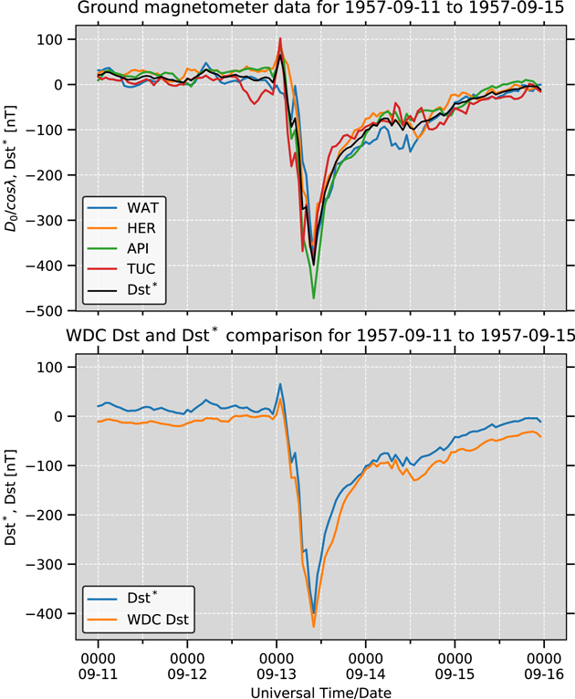
Figure 3. Comparison of the standard Dst index and our Dst* estimate for the 1957 September storm. For the Dst* estimate, we have used WAT, HER, API, and TUC.
Download figure:
Standard image High-resolution imageOur Dst* estimate and the hourly disturbance at each observatory with latitudinal weighting have been summarized in Figure 4. Our reconstruction shows its intensity in the minimum Dst* estimate of ≈−464 nT. The reconstructed time series shows a positive excursion peaked at 79 nT at 05 GMT after the ICME arrival at 03:57 GMT, probably because of the combination with the second SSC at 05:19 GMT reported at Hermanus (Ogg 1941). Afterward, this storm shows an initial negative excursion down to −180 nT at 09 GMT with temporal recovery to −64 nT at 12 GMT. The magnetic field was exposed to a steep decrease at 15 GMT and then peaked to −464 nT at 16 GMT on March 1 and a gradual recovery phase up to early March 3. This "two-step" time series is consistent with the frequent geomagnetic behavior in major geomagnetic storms (Kamide et al. 1998), resulting from variable IMF, a combination of shock-sheath and following magnetic cloud, or a combination of multiple ICMEs (Daglis et al. 2003; Richardson & Zhang 2008; Lugaz et al. 2016). Near the first negative dip, the Di (t)/cos λ value decreased steeper at API than at HER. This can be attributed to the asymmetric development of the storm-time ring current (Cummings 1966), in which the intensity of the storm-time ring current is highest in the dusk-midnight sector, whereas it is lowest in dawn-noon sector. The in situ observation shows that the asymmetry is prominent during the storm main phase because fresh ions are transported from the nightside plasma sheet to the duskside by the enhanced magnetospheric convection (Ebihara et al. 2002). During the recovery phase, the asymmetry is relaxed because of the dominance of the westward grad-B and curvature drift motion of the ions (Ebihara et al. 2002). Note that the API magnetogram has a data gap on March 2 in UT, whereas this data gap falls in the gradual recovery phase and hence does not affect our intensity reconstruction. In fact, our Dst* estimate curve (continuous black curve) and one without API data (broken black curve) are shown in Figure 4. Closer inspection shows that, at Tucson, "At about 16 h the H-reserve spot went off scale negative for a range in H in excess of 550 gammas" (White 1941, p. 257), whereas its hourly data are without break. Therefore, it is probable that Tucson magnetogram went off scale for a short time and made the hourly value slightly more conservative than the reality. Therefore, we consider our intensity estimate to be a conservative estimate and describe its intensity as minimum Dst* ≤ −464 nT.
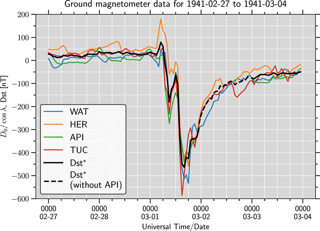
Figure 4. The Dst* estimate and the individual disturbance time series at each reference station for 1941 February 27–March 3. The Dst* estimate is shown in a continuous black curve (except for March 2) and a broken black curve on March 2 without API data. The corrected time series of WAT, HER, API, and TUC are shown in blue, orange, green, and red, respectively.
Download figure:
Standard image High-resolution image5. Low-latitude Aurorae
Around its peak recorded at 16 GMT on March 1, the East Asian sector was favorably situated in the midnight sector for the auroral visibility. Indeed, the aurorae have been reported in Manchuria and northern Japan at that time. In Manchuria, aurorae were reported at Hǎilāěr (N49°13', E119°46'; 378 MLAT) during 23:05 (March 1)–00:18 (March 2) in LT and 01:40–02:20 (March 2) in LT, namely 15:05–16:18 and 17:40–18:20 (March 1) in GMT. The aurorae were reported as reddish glows moving from NW to E in the first part and then as reddish glows with stripes moving from NE to NW in the second part (Shèngjng Shíbào, 1941-03-08, p. 4). This implies that the aurora moved eastward in the premidnight, and westward in the postmidnight. Its motion is, in part, consistent with low-latitude aurorae, in which the eastward motion and the westward motion were observed in the duskside (Shiokawa et al. 1994).
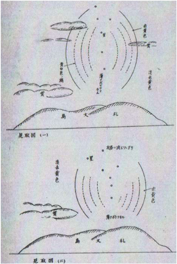
In northern Japan, aurorae were reported on both sides of Soya Strait. At Otomari (N46°38', E142°46'; 365 MLAT), the aurorae were reported during 23:00 (March 1)–03:55 (March 2) in LT (14:00–18:55 on March 1 in GMT), as reddish glow with various intensities. At Wakkanai (N45°25', E141°40'; 352 MLAT), diffuse reddish aurorae were visible during 22:56 (March 1)–04:30 (March 2) in LT (13:56–19:30 on March 1 in GMT). At its maximum, the aurora altitude reached almost up to the zenith. At Oshidomari (N45°14', E141°13'; 350 MLAT), reddish-yellow glow with stripes in bluish-white was visible during 01:05–03:30 (March 2) in LT (16:05–18:30 on March 1 in GMT) and its altitude reached up to 60–70° at its maximum (Kisho Yoran 1941, pp. 267–269; see Figure 5).
Figure 5. Japanese auroral sketches at Oshidomari reproduced from Kisho Yoran (1941, p. 268) with a reddish-yellow background and bluish-white stripes at its maximum (top) and after its decay (bottom). The bluish-white stripes are shown in broken lines. The reddish-yellow glows are shown in the background sky. The island depicted below is Rebun Island northward from Oshidomari.
Download figure:
Standard image High-resolution image
The auroral visibility in the East Asian sector lasted ≈14–18.5 GMT and is chronologically consistent with the main phase of this geomagnetic storm. In addition, a short telegraph disturbance was reported at Oshidomari during 01:55–02:05 on March 2 in LT (16:55–17:05 GMT on March 1) and this is chronologically located immediately after the peak of this storm at 16 GMT on March 1 (Kisho Yoran 1941, pp. 267–269).
Among these records, those at Wakkanai at 352 MLAT and Oshidomari at 350 MLAT provide the elevation angle of the auroral visibility almost up to the zenith and up to 60–70°, respectively. On their basis, the equatorward boundary of the auroral oval (EBAO) is estimated 376 and 385 in invariant latitude (ILAT) in terms of footprints of the magnetic field lines, assuming the auroral altitude as ≈400 km (Roach et al. 1960; Ebihara et al. 2017). These values almost coincide with one another. The slight equatorward extension in the former may be tentatively associated with the different extension of the SAR (stable auroral red) arcs and reddish aurorae. This is because SAR arcs typically do not have visible structure (Kozyra et al. 1997) and are consistent with the Wakkanai report having a diffuse reddish glow. On the other hand, what was described in the Oshidomari report is certainly an auroral display, being described as a reddish glow with stripes respectively (Kisho Yoran 1941, pp. 267–269).
6. Conclusion and Discussion
In this contribution, we have analyzed the time series of the extreme space weather event in 1941 February–March. Despite the lack of optical evidence of the source solar flare, contemporary magnetograms have shown significant magnetic crochets (ΔH ≈ ∣35∣ nT at Abinger) at 09:29–09:38 GMT on February 28. This is synchronized with a significant polar cap absorption lasting for 4 days since February 26/27 and probably associated with a notable solar proton event.
The driving ICME impact was recorded with SSCs at 03:57–03:59 GMT on March 1 (Table 1). On their basis, the ICME speed has been computed as 2260 km s−1. By applying well-known empirical models for the solar wind dynamic pressure and the magnetopause standoff position at the instance of maximum compression, it was found that they are 4.9 nPa and 7.2 RE, respectively. This calculated average ICME speed ranks the ICME as being the fourth fastest on record following those in 1972 August, 1859 September, and 1946 February (Cliver et al. 1990; Cliver & Svalgaard 2004; Gopalswamy et al. 2005; Knipp et al. 2018; Chertok 2020). This subsequent geomagnetic activity may have been caused by the CME sheath and/or magnetic cloud (Lugaz et al. 2016; Kilpua et al. 2019).
We have reconstructed its time series and intensity (minimum Dst* ≤ −464 nT at 16 GMT on 1941 March 1) based on the hourly magnetic measurements at Hermanus, Watheroo, Apia, and Tucson. Our intensity estimate has placed this storm in an extreme category, as only five geomagnetic storms exceeded the threshold of Dst = −400 nT during the space age, for the last 64 years (e.g., Meng et al. 2019). Indeed, this intensity is more extreme than the second most intense storm in 1959 July (minimum Dst = −429 nT) but considerably less than the most intense storm in 1989 March (minimum Dst = −589 nT), within the standard Dst index since the IGY (WDC for Geomagnetism at Kyoto et al. 2015). While this storm is slightly more moderate than historical superstorms in 1859 September, 1872 February, 1903 October/November, 1909 September, 1921 May, and 1946 March (Cliver & Dietrich 2013; Hayakawa et al. 2018a, 2019a, 2019b, 2020b, 2020a, 2020c; Love et al. 2019a, 2019b), its intensity is significantly notable and in modern times its consequences would be quite serious.
With its peak around 16 GMT, the East Asian sector was favorably situated for the auroral observations. Indeed, the East Asian auroral records imply the EBAO as 385 ILAT. The temporal and spatial evolution of the auroral oval compares well with the magnetic disturbances in the high- resolution British magnetograms (Figure 2). From the first SSC at 03:58 GMT, the vertical components (Bz) at each of the British operated observatories appear to be broadly coherent. From 13:30–14:30 GMT, Lerwick witnessed a sharp decrease in Bz with a simultaneous increase in the horizontal component (BH), while Abinger and Eskdalemuir witnessed a large increase in Bz, and a staggered increase in BH. This most likely indicates that an eastward Hall current flew broadly in the ionosphere over Lerwick (626 MLAT) and Eskdalemuir (586 MLAT) (Rostoker & Kisabeth 1973). After 14:30 GMT, the broadly coherent variations between the Eskdalemuir and Lerwick Bz suggests that the eastward Hall current had moved southward of Eskdalemuir. The minimum reported Bz for Abinger in Jones (1954) may indicate that the eastward ionospheric current went southward beyond Abinger (530 MLAT) by 16:30 GMT. Around this time, Abinger saw large positive BH variations, indicating the proximity of auroral currents. From 17:10 GMT onwards, the Bz at Abinger is anticorrelated with Lerwick and Eskdalemuir, again indicating an eastward ionospheric current between Eskdalemuir and Abinger, until around 20:30 GMT, when the geomagnetic activity begins to gradually subside at all sites.
On the other hand, Hermanus shows characteristics of the ring current instead of ionospheric currents. This indicates that Lerwick was at one point probably near the poleward boundary of the auroral oval, Eskdalemuir and Abinger were almost under the auroral oval except for the storm maximum, and the auroral oval probably extended more equatorward than Abinger around the maximum. The auroral oval likely did not reach latitudes low enough to affect measurements at Hermanus in the Southern Hemisphere. Assuming that the evolution of the auroral ovals in both hemispheres were similar to one another, this time series agrees with the maximum of the auroral activity around 16 GMT and its spatial evolution of  ILAT, situated between MLATs of Abinger (
 MLAT) and Hermanus (
 MLAT).
This temporal evolution compares the auroral expansion with those during the 1903 October/November storm (minimum Dst* ≈ −531 nT versus EBAO ≈ 441 ILAT; Hayakawa et al. 2020b), the 1946 March storm (minimum Dst* ≤ −512 nT versus EBAO ≤ 418 ILAT; Hayakawa et al. 2020a), and the 1989 March storm (minimum Dst = −589 nT versus EBAO ≈ 35–401 ILAT; Rich & Denig 1992; Boteler 2019). As such, this auroral expansion is certainly not as extreme as those during the superstorms in 1859 and 1921 (minimum Dst* ≈ −900 nT; Cliver & Dietrich 2013; Love et al. 2019b; Hayakawa et al. 2019a) but still are comparable with those around the minimum Dst* ≈ −500 nT.
Interestingly, as shown in Table 1, the reported amplitudes of geomagnetic disturbance in spot value are more significant at the equatorial stations (1180 nT at Huancayo and >785 nT at Alibag) than at midlatitude stations (>550 nT at Tucson and 614 nT at Hermanus), while the lost value with the magnetogram saturations still reserve the possibility of local extreme disturbances at midlatitude stations. This is comparable with the trend seen in the 1946 March storm, where the equatorial magnetograms showed more significant disturbances than the midlatitude magnetograms (Table 1 of Hayakawa et al. 2020a). The contrast of the minimum Dst* ≤ −464 nT with Huancayo spot value = 1180 nT casts serious caveats on existing discussions of the 1859 geomagnetic superstorms with spot value at the single equatorial station (e.g., Tsurutani et al. 2003), and requires investigations of further midlatitude magnetograms to improve its intensity estimate.
This work was supported in part by JSPS Grants-in-Aid JP15H05812, JP17J06954, JP20K22367, JP20K20918, and JP20H05643 JSPS Overseas Challenge Program for Young Researchers, the 2020 YLC collaborating research fund, and the research grants for Mission Research on Sustainable Humanosphere from Research Institute for Sustainable Humanosphere (RISH) of Kyoto University and Young Leader Cultivation (YLC) program of Nagoya University. We thank Mt. Wilson Observatory for providing sunspot drawings on 1941 February 27, WDC for Geomagnetism at Edinburgh for providing geomagnetic baselines and British magnetograms, WDC for Geomagnetism at Kyoto for providing the Dst index and magnetic measurements at Hermanus, San Juan, Honolulu, and Watheroo, Kakioka Event Database for providing data on the SSC and magnetic storms observed in the said observatory, WDC SILSO for providing international sunspot numbers, and Solar Science Observatory of the NAOJ for providing copies of Quarterly Bulletin on Solar Activity. Magnetograms were digitized using the WebPlotDigitizer software (https://automeris.io/WebPlotDigitizer/). S.P.B. was supported by the NASA's Living With a Star program (17-LWS17_2-0042). H.H. thanks Margaret A. Shea for her helpful advice on the historical solar proton events.
Footnotes
- 12
- 13
- 14
- 15