


Abstract
Visible coronal structure, in particular the spatial evolution of coronal streamers, provides indirect information about solar magnetic activity and the underlying solar dynamo. Their apparent absence of structure observed during the total eclipses throughout the Maunder minimum has been interpreted as evidence of a significant change in the solar magnetic field from that during modern solar cycles. Eclipse observations available from the more recent Dalton minimum may be able to provide further information, with sunspot activity being between the levels seen during recent solar cycles and in the Maunder minimum. Here, we show and examine two graphical records of the total solar eclipse on 1806 June 16, during the Dalton minimum. These records show significant rays and streamers around an inner ring. The ring is estimated to be ≈0.44 R⊙ in width and the streamers in excess of 11.88 R⊙ in length. In combination with records of spicules or prominences, these eclipse records visually contrast the Dalton minimum with the Maunder minimum in terms of their coronal structure and support the existing discussions based on the sunspot observations. These eclipse records are broadly consistent with the solar cycle phase in the modeled open solar flux and the reconstructed slow solar wind at most latitudes.
Export citation and abstract BibTeX RIS
1. Introduction
Variability of the solar magnetic field has been directly monitored for ≈4 centuries with sunspot observations as a visual manifestation of magnetic flux (Clette et al. 2014; Arlt & Vaquero 2020). These observations show the regular Schwabe cycles of ≈11 yr and two longer-term intervals with significantly suppressed solar activity: most prominently, the Maunder minimum (hereafter, MM; circa 1645–1715) and, to a somewhat lesser extent, the Dalton minimum (hereafter, DM; circa 1797–1827) (Hathaway 2015; Muñoz-Jaramillo & Vaquero 2019). While a number of additional intervals with comparable solar activity have been identified over millennial timescales using proxy reconstructions with the cosmogenic isotopes (Usoskin et al. 2007; Inceoglu et al. 2015), only the MM and DM can be investigated with direct observations and measurements (Usoskin et al. 2015; Hayakawa et al. 2020).
The physical natures of these two intervals, the MM and the DM, are of great interest as grand minima are generally associated with a special state of the solar dynamo (Charbonneau 2020). Analyses of these intervals are difficult, due to their poor observational coverage and different observational motivations relative to the modern era (Arlt & Vaquero 2020). Nevertheless, thorough analyses of the original observations have revealed their differences in terms of their solar-cycle amplitude and length, as well as sunspot distributions and highlighted their probable difference, although the poor observational coverage still prevents definitive conclusions (Eddy 1976; Ribes & Nesme-Ribes 1993; Usoskin et al. 2015; Hayakawa et al. 2020) and even accommodates discussions of the possibility of one solar cycle lost just before the onset of the DM (Usoskin et al. 2009; Karoff et al. 2015; Owens et al. 2015; Vaquero et al. 2016; Hayakawa et al. 2018).
In this regard, the solar coronal structure is of significant interest, forming a visual representation of the large-scale solar magnetic field, and with the solar coronal holes providing a visual estimate of the extent of the fast solar wind source regions. In the typical solar cycles of the modern era, the polar coronal holes reach maximum areal extent around the minima to concentrate the coronal streamers nearer the solar equator, whereas the polar coronal holes shrink and even disappear around the maxima, with streamers extending to all latitudes. As such, they serve as a basis to reconstruct the large-scale solar magnetic field and hence that of the global solar wind (e.g., Loucif & Koutchmy 1989; Vaquero 2003; Marsch 2006; Lockwood & Owens 2014; Hathaway 2015; Owens et al. 2017; Pasachoff et al. 2017).
Both the MM and DM occurred long before the use of artificial coronagraphs which can reveal the coronal structure by blocking the bright solar disk. Such structures, however, can be revealed during total solar eclipses, when the Moon entirely hides the Sun and shuts out most of its brightness. On such occasions, the brightness of the coronal streamers is visually captured (Eddy 1976; Woo 2019) and their extent provides valuable insight on the large-scale solar magnetic field (Owens et al. 2017). The visual corona, as in unpolarized light, is a mixture of electron-scattered K-corona and dust-scattered F-corona. As such, extension of the K-corona is constrained by the structured solar magnetic field but F-corona appears structureless, free from such constraints.
Therefore, the coronal structure of the MM has attracted much scientific interest. Contemporary eclipse records have been intensively investigated and have shown the halo-shaped corona without significant streamer structure (Eddy 1976; Riley et al. 2015). Eddy (1976) speculated about a total loss of the solar magnetic field during the MM. Conversely, the continuation of solar cycles has been inferred from sunspot records and cosmogenic isotopes (Beer et al. 1990, 1998; Usoskin et al. 2001, 2015; Cliver & Ling 2011; Lockwood et al. 2011; Owens et al. 2012; Cliver et al. 2013; Vaquero et al. 2015) and a report of a solar spicule or prominence during the 1706 eclipse (Foukal & Eddy 2007) shows that the large-scale solar magnetic field survived, even if its magnitude was greatly diminished (Cliver & Ling 2011; Riley et al. 2015).
In this context, the coronal structure in the DM is also of significant interest. However, eclipse reports in this period (circa 1797–1827) have yet to be analyzed with a view to understanding the large-scale solar magnetic field. Fortunately, this interval hosted significant developments in scientific understanding for the solar corona, when José Joaquín de Ferrer (1809) recorded the total eclipse on 1806 June 16. It was the extended nature of the glow around the eclipsed Sun that made the previously hypothesized association with an extended lunar atmosphere highly unlikely. From the work of de Ferrer the name "corona" was established, as was the fact that it was part of the Sun (Vaquero & Vázquez 2009). Moreover, de Ferrer was not a lone observer. Simeon de Witt (1809) also observed this eclipse and cited another graphical record. Situated in the midst of the DM, these records provide valuable visual evidence for the large-scale solar magnetic field. Therefore, we have conducted investigations on the eclipse records at that time, evaluated the reported coronal extents, and compared them with contemporary observations of sunspot number, as well as modeled reconstructions of the open solar flux, heliospheric modulation potential, and solar wind speed as a function of latitude and time.
2. Observations
The total eclipse on 1806 June 16 started from the coast of California, came across the central United States and the northern Atlantic Ocean, and ended in Western Africa. Figure 1 shows its totality path, assuming the ΔT (difference of the terrestrial time and universal time) as 16.3 s (Stephenson et al. 2016). As shown here, New England was favorably situated in this totality path and two notable eclipse drawings were recorded for this eclipse (see Figure 2).
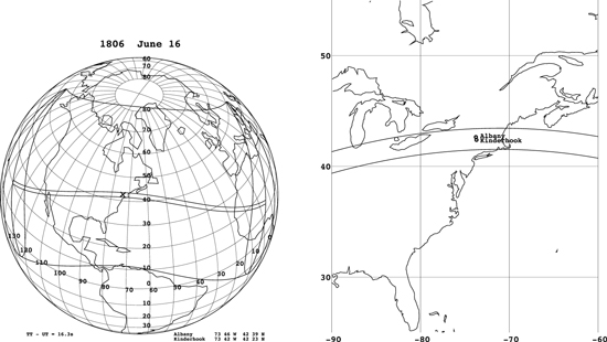
Figure 1. Totality path of the total eclipse on 1806 June 16, assuming the ΔT = 16.3 s (Stephenson et al. 2016) and its enlargement in the Eastern Coast of the United States. Albany and Kinderhook are marked in these maps.
Download figure:
Standard image High-resolution image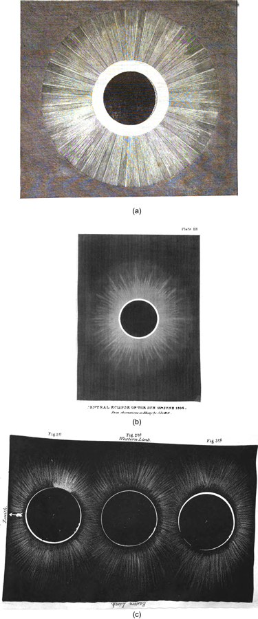
Figure 2. Total eclipse drawings of 1806 June 16; (a) Don José Joaquín de Ferrer's eclipse drawing reproduced from de Ferrer (1809, Plate VI, Figure 1); (b), (c) Ezra Ames's eclipse drawings reproduced from de Witt (1852, Plate 3).
Download figure:
Standard image High-resolution imageThe first drawing is an original drawing of Don José Joaquín de Ferrer at Kinderhook (N42°23', W73°42'; see Figure 2(a)), which has been often mentioned in the scientific literature (Todd 1894; Vaquero & Vázquez 2009). The drawing slightly emphasizes the eclipsed Sun more than its deformed reproduction in Todd (1894, p. 115), which has been more often cited than the original version. De Ferrer used an achromatic telescope, a circle for reflection, an Arnold chronometer, and a darkened glass (de Ferrer 1809, pp. 265–266). He described the eclipse thus, "the disk had round it a ring or illuminated atmosphere, which was of a pearl colour, and projected 6' from the limb, the diameter of the ring was estimated at 45'. ... From the extremity of the ring, many luminous rays were projected to more than 3 degrees distance. The lunar disk was ill defined, very dark, forming a contrast with the luminous corona; with the telescope I distinguished some very slender columns of smoke, which issued from the western part of the moon. The ring appeared concentric with the Sun, but the greatest light was; in the very edge of the moon, and terminated confusedly at 6' distance. [At] 11:00, [I] observed the appearance of a ribbon or border, similar to a very white cloud, concentric with the Sun, and which appeared to me to belong to its atmosphere, 90° to the left of the moon." (de Ferrer 1809, pp. 266–267.)
He emphasized the luminous ring around the eclipsed Sun: "Figure 1 in Plate VI (NB our Figure 2(a)), represents the total eclipse, I shall only remark, that the luminous ring round the moon, is exactly as it appeared in the middle of the eclipse, the illumination which is seen in the lunar disk, preceded 6'' 8 the appearance of the first rays of the Sun" (de Ferrer 1809, p. 274). "It has appeared to me, that the cause of the illumination of the moon, as noticed above, is the irradiation of the solar disk, and this observation may serve to give an idea of the extension of the luminous corona of the Sun" (de Ferrer 1809, p. 275).
This eclipse was also observed at Albany (N42°38'42'', W73°46'), where Ezra Ames painted and Simeon de Witt recorded its detail (Worth 1866, p. 41). Ezra Ames was "an eminent portrait painter," as described by de Witt (1809, p. 300). His drawing was attached to de Witt (1809) and deposited in the Hall of the American Philosophical Society. Later on, his drawing has been involved in de Witt (1852, Plate 3) with a sequence of drawings, as shown in Figures 2(b) and (c).
3. Results
These diagrams look consistent with each other, showing a brighter inner ring and the outer luminous rays or streamers all around the eclipsed Sun. Indeed, de Witt (1809, p. 300) emphasized its similarity with de Ferrer's drawing at Kinderhook. Observing from the same town, de Witt (1809) described his observations as: "The edge of the moon was strongly illuminated, and had the brilliancy of polished silver. No common colors could express this; I therefore directed it to be attempted as you will see, by a raised silvered rim, which in a proper light, produces tolerably well, the intended effect" (de Witt 1809, p. 300); and "The luminous circle on the edge of the moon, as well as the rays which were darted from her, were remarkably pale, and had that bluish tint, which distinguishes the color of quick-silver from a dead white" (de Witt 1809, p. 301). de Witt's description of the color is interesting as it fails to mention any red color, which had been reported in the 1706 eclipse by Captain Stannyan and which reveals magnetic field in the chromosphere (see Foukal & Eddy 2007).
The extent of the eclipse features is detailed in de Ferrer's report, along with their characteristics. The brighter inner ring reportedly extended ≈6' with a color of silver or pearl. The luminous rays had dimmer color and reportedly extended from the inner ring with a distance of ≥3°. Although slightly stylized, their illustrations show the bright inner ring and the outer radiation (Figure 2). The breadth of the outer radiation is particularly notable. The inner and outer rings are probably best interpreted as lower solar atmosphere and the outer corona with streamers, respectively. Moreover, de Ferrer's description on "very slender columns of smoke, which issued from the western part of the moon" implies his observations on prominences or solar spicules (see, e.g., Pettit 1943; Beckers 1968; Mackay et al. 2010).
The detailed reports on the visual extents of the inner ring and outer rays allow us to estimate their absolute extents. During the 1806 eclipse, the distances of the Sun and the Moon from Kinderhook were estimated as ≈1.0161892 au and ≈0.0023920 au with JPL DE430. Hence solar radius R⊙ and lunar radius would span 15'44'' and 16'42'' in the sky, respectively. The maximal magnitude6 at Kinderhook is calculated as ≈1.028, whereas this is calculated as ≈1.030 at the center-line near Kinderhook. Accordingly, the reported extent of the inner ring of ≈6' from the lunar disk implies its absolute extent from the solar disk as ≈0.44 R⊙, considering the difference of lunar and solar radii of 58''. Likewise, the reported extent of the outer rays of ≥3° from the limb of this inner ring implies its absolute extent as ≥11.88 R⊙.
4. Discussion
One of the striking common features of the eclipse reports is the coronal streamers all around the eclipsed Sun, captured both descriptively and graphically (Figure 2). This feature agrees well with the solar-maximum-type coronal structure (see, e.g., Figure 1 of Owens et al. 2017). This supports the existence of a substantial K-corona and hence large-scale solar magnetic field, even in the midst of the DM, unlike the records of the eclipse during the MM (Eddy 1976; Riley et al. 2015). On this basis, the DM could be considered in a similar state of the solar dynamo, only with reduced amplitude in comparison with the modern solar cycles, unlike the MM (e.g., Riley et al. 2015). This interpretation agrees with the existing discussion of the amplitude and duration of the solar cycles, as well as the sunspot distributions in the DM (Hayakawa et al. 2020), in comparison with those of the MM (Eddy 1976; Ribes & Nesme-Ribes 1993; Usoskin et al. 2015).
As shown in Figure 3, this eclipse occurred in the declining phase of SC 5, which peaked in 1805 February in smoothed monthly mean (Hathaway 2015) of the international sunspot number (Clette et al. 2014; Clette & Lefèvre 2016, see Figure 3) as well as sunspot positions in Derfflinger's observations (Hayakawa et al. 2020). This was also the case with frequency of reported mid-latitude aurorae in the European sector, on which basis John Dalton first noted the existence of this secular minimum and after whom it was subsequently named7 (Dalton 1834; Silverman 1992). In fact, it is shown that auroral visibility generally moved poleward, both when compiling the existing auroral reports in the European sector, as well as those from islands in the Northeastern Atlantic Ocean (Lockwood & Barnard 2015; Vázquez et al. 2016).
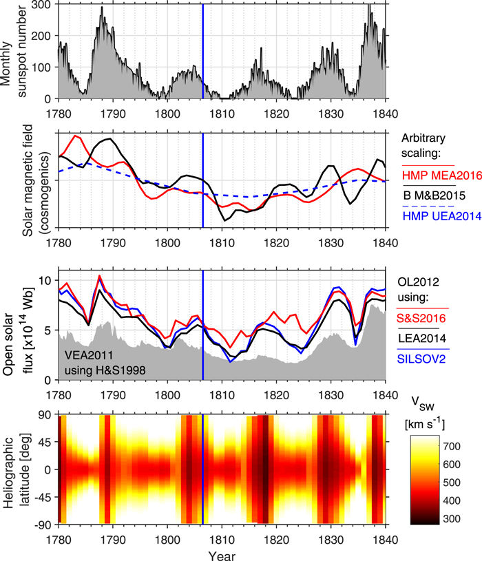
Figure 3. Summary of observed and modeled solar properties through the Dalton minimum. The 1806 eclipse is shown as the blue vertical line. First panel: monthly sunspot number (Clette & Lefèvre 2016). Second panel: the colored lines show estimates of solar activity, scaled for plotting purposes: HMF B from 10Be (McCracken & Beer 2015; Owens et al. 2016b; black), annual (red) and decadal (blue) heliospheric modulation potential from 14C (Usoskin et al. 2014; Muscheler et al. 2016). Third panel: reconstructed open solar flux based on the OL model (Owens & Lockwood 2012), applied to different sunspot series: red = Svalgaard & Schatten (2016), black = Lockwood et al. (2014), and blue = SILSO V2 (Clette & Lefèvre 2016). Thus the red and the black curves correspond to the "high" and "low" scenarios in Asvestari et al. (2017). The gray-shaded region is the modeled OSF from Vieira et al. (2011), based on HS98. Fourth panel: the reconstructed solar wind speed as a function of heliographic latitude and time (Owens et al. 2017).
Download figure:
Standard image High-resolution imageSimilar trends are found in centennial-scale reconstructions of solar activity based on a number of diverse sources. Cosmogenic isotopes, such as 14C and 10Be, can be used to estimate the time history of galactic cosmic ray (GCR) intensity reaching Earth, and thus the ability of the solar magnetic field to deflect GCRs (e.g., Beer et al. 2012; Usoskin 2017). This shielding ability is quantified by the heliospheric modulation potential (HMP). The shielding is actually caused by scattering of the GCRs by irregularities in the heliospheric field, but their net effect is well quantified by the open solar flux (OSF), the total solar magnetic flux which extends to the top of the solar atmosphere and fills the heliosphere and so acts as a barrier to GCRs. The faster deposition time of the 10Be cosmogenic isotope, and the fact that it is not subsequently exchanged between different reservoirs, means that solar activity can potentially be resolved at annual timescales. However, a number of caveats apply in the interpretation of these data. The signal-to-noise in the 10Be records, coupled with the complexity of converting 10Be concentration into a measure of solar magnetism means that at annual resolution the reconstructions contain uncertainties of the order ±2 yr in timing and around 25% in magnitude (Owens et al. 2016b). The red and blue lines in the second panel of Figure 3 show the annual HMP estimate from Muscheler et al. (2016) and decadal HMP estimate from Usoskin et al. (2014), while the black line shows the B (the near-Earth heliospheric magnetic field intensity, closely related to the OSF; see Figure 10 of Lockwood et al. 2014) estimate from McCracken & Beer (2015), filtered in the same way as Owens et al. (2016b). While the same long-term trends are present in all cosmogenic estimates of solar activity, the annual reconstructions show less agreement about the timing and magnitude of individual cycles (see, e.g., Beer et al. 1990; Berggren et al. 2009).
OSF and near-Earth heliospheric field, B, can also be estimated from sunspot records by assuming sunspots represent the source of new OSF and that OSF can be treated as a continuity equation (Solanki et al. 2000). This method has very good agreement with geomagnetic reconstructions over the interval 1845–2013 (Owens et al. 2016a). Of course, there may be long-term drifts in the calibration of the sunspot record before this period (from changes in observing capability, intercalibration of different observers, etc.; see Clette et al. 2014; Clette & Lefèvre 2016), which makes the independent estimates of cycle amplitude from 14C and 10Be very useful. However, the timing of sunspot cycles, and hence features in the subsequent OSF reconstruction, likely accommodate uncertainty of a few years for the epoch of DM (Adolphi & Muscheler 2016).
The third panel of Figure 3 shows that the OSF from the model constrained by the sunspot number did not peak until mid-1806, when this eclipse took place. Here, the OL12 model (Owens & Lockwood 2012) has been applied to different sunspot series: Svalgaard & Schatten (2016), Lockwood et al. (2014), and SILSO V2 (Clette & Lefèvre 2016), shown in red, black, and blue curves, respectively. The red and the black curves thus correspond to the "high" and "low" scenarios in Asvestari et al. (2017). These reconstructions are compared with the gray-shaded region, which is the modeled OSF from Vieira et al. (2011), based on the SATIRE-T model applied to the group sunspot number of Hoyt & Schatten (1998; HS98). All these OSF reconstructions are unsigned flux. Here, the OSF from Vieira et al. (2011) shows a slightly lower value in comparison with other curves with the OL12 model, as the HS98 series used in Vieira et al. (2011) shows a larger trend between 1800 and now than the other series used in the OL12 model (Lockwood et al. 2014; Svalgaard & Schatten 2016; SILSO V2), as shown in Figure 11 of Clette & Lefèvre (2016).
Further information about the expected structure of the corona and solar wind can be estimated by assuming new OSF is produced in the streamer belt, resulting in slow wind, which then gradually transitions into coronal hole flux, resulting in fast solar wind (Lockwood & Owens 2014). The time constant for this transition is a free parameter determined by comparison with 40 yr of photospheric magnetic field observations and models (see Owens et al. 2017). The resulting solar wind structure as a function of latitude and time is shown in the fourth panel of Figure 3. On this basis, the eclipse occurrence in mid 1806 took place during an interval with slow wind at most latitudes, suggesting streamers should extend to most latitudes (Owens et al. 2014). This is broadly consistent with the eclipse images (Figure 2), which showed streamers all around the eclipsed Sun. As such, these two eclipse drawings in 1806 June confirm the validity of the existing models of Owens et al. (2017) within the DM in terms of their reconstructions of OSF phase and solar-wind speed as a function of latitude and time.
5. Conclusion
In this article, we have examined the total eclipse drawings on 1806 June 16 and visually confirmed the activity phase of the solar magnetic field in the midst of the DM. Both of de Ferrer's and Ames's eclipse drawings showed corona with significant rays and streamers. On the basis of de Ferrer's report, we computed the extent of the outer rays and the inner ring from the solar disk as ≥11.88 R⊙ and ≈0.44 R⊙, respectively. De Ferrer's report also implies the presence of prominences or solar spicules. These details confirm the presence of the solar and heliospheric magnetic fields in the midst of the DM.
This marks a significant difference from the coronal structure during the MM, when streamers were apparently missing or at least not bright enough to be visible and the corona was recorded without significant structure (Eddy 1976; Riley et al. 2015). This contrast visually shows significant difference of the DM with the MM in terms of their background state of the solar dynamo, and robustly supports the existing discussions on the difference of the DM and MM on the basis of their sunspot positions and amplitude and duration of their solar cycles (Usoskin et al. 2015; Hayakawa et al. 2020). This comparison disproves postulates that the MM was no more than an extended version or equivalence of the DM such that both are similar minima of the quasi-regular Gleissberg cycle (Zolotova & Ponyavin 2015). This strongly supports what has been discussed and analysed by Usoskin et al. (2015) based on a variety of other historic and paleo-data sets.
Moreover, comparison of these eclipse drawings is broadly consistent with the modeled reconstruction on the cycle phase of OSF and on that on the solar wind speed as a function of latitude and time. The OSF peaked around this eclipse and the slow solar wind extended to most latitudes, suggesting streamers should also extend to most latitudes. This coincidence confirms the validity of the existing model of Owens et al. (2017) even in the midst of the DM.
We thank Ken'ichi Fujimori for his advice on the coronal visibility during the total eclipses in 1991 and 2009, WDC SILSO at Royal Observatory of Belgium for providing international sunspot number and its regular maintenance, Joe DiLullo and other archivists in American Philosophical Society Archives for their advices on the eclipse reports, Sam M. Silverman for letting us know the background history on how the Dalton Minimum was named, and Raimund Muscheler for providing the background data in Muscheler et al. (2016). We thank Ilya G. Usoskin for providing background data for Vieira et al. (2011) and Usoskin et al. (2014), and Shin Toriumi for his helpful discussions and suggestions. H.H. was partially funded by the Young Leader Cultivation (YLC) program of Nagoya University, the 2020 Collaborative Research Grants for YLC, Institute for Advanced Reseraches of Nagoya University, research grant for Exploratory Research on Sustainable Humanosphere Science from Research Institute for Sustainable Humanosphere (RISH) of Kyoto University, the Unit of Synergetic Studies for Space of Kyoto University, BroadBand Tower, and JSPS grant-in-aids (JP15H05812, JP15H05816, and JP20K20918). M.O. was partially funded by Science and Technology Facilities Council (STFC) grant No. ST/R000921/1. This work has been partly merited from participation in the International Space Science Institute (ISSI, Bern, Switzerland) via the International Team 417 "Recalibration of the Sunspot Number Series".
Footnotes
- 6
Here the magnitude of eclipse is defined by (R⊙ +
 − d)/(2 R⊙), where R⊙ is the apparent angular radius of the Sun, is the apparent angular radius of the Moon, and d is the apparent angular distance between the centers of the Sun and the Moon. In the case of partial solar eclipses the magnitude is equal to the fraction of the Sun's diameter obscured by the Moon. In the case of total solar eclipses the magnitude is equal to 1 at the instants of the beginning and end of the total solar eclipses and varies continuously with time.
 - 7
It is Sam M. Silverman who suggested this term during his discussion with Jack Eddy and George Siscoe (S. M. Silverman 2020, private communication).

