Anisotropic Radio-wave Scattering and the Interpretation of Solar Radio Emission Observations

Solar radio emission is produced in the turbulent medium of the solar atmosphere, and its observed properties (source position, size, time profile, polarization, etc.) are significantly affected by the propagation of the radio waves from the emission site to the observer. Bright radio emission produced in the outer solar corona during flares is mostly produced via plasma emission mechanisms, so that the radiation is generated close to the plasma frequency or its harmonic (see, e.g., Suzuki & Dulk 1985; Pick & Vilmer 2008 for reviews). Since the refractive index of an unmagnetized plasma ${n}_{\mathrm{ref}}={(1-{\omega }_{{pe}}^{2}/{\omega }^{2})}^{1/2}$ is significantly different from unity for ω close to ω_pe, the effects of density inhomogeneity along the wave path play a particularly strong role in the propagation of solar radio bursts produced by plasma processes. Appreciating this fact, even early observations (e.g., Wild et al. 1959; Smerd et al. 1962; Steinberg et al. 1971) considered radio-wave escape to be an important effect.

Scattering of radio waves on random density irregularities has long been recognized as an important process for the interpretation of radio source sizes (e.g., Steinberg et al. 1971), positions (e.g., Fokker 1965; Stewart 1972), directivity (e.g., Thejappa et al. 2007; Bonnin et al. 2008; Reiner et al. 2009), and intensity-time profiles (e.g., Krupar et al. 2018). In the particularly strong scattering environment appropriate for electromagnetic waves close to the plasma frequency, the wave direction is quickly randomized, and the waves quickly become isotropic. As the waves propagate farther away from the source, large-scale refraction also produces a degree of focusing/defocusing. The observed properties of solar radio emission are therefore determined by an interconnected combination of scattering off small-scale inhomogeneities, which generally shifts the observed positions of sources away from the solar disk center (Riddle 1972; Gordovskyy et al. 2019), and refraction by relatively large-scale density inhomogeneities, such as coronal mass ejection fronts (Afanasiev 2009) or coronal streamers and fibers (Bougeret & Steinberg 1977), which generally shifts the sources toward the disk center (Wild et al. 1959; Smerd et al. 1962; Steinberg et al. 1971).

Subarcminute imaging observations of Type III solar radio bursts have shown that intrinsic sources with sizes ≲01 result in observed sources as large as ∼20' at 30 MHz (Kontar et al. 2017; Sharykin et al. 2018), demonstrating that scattering dominates the properties of observed source sizes. Moreover, the locations of the upper and lower subband sources of Type II solar radio bursts are observed to be spatially separated (e.g., Zimovets et al. 2012; Chrysaphi et al. 2018), with the amount of separation being consistent with radio-wave scattering of plasma radio emission from a single region (Chrysaphi et al. 2018).

The majority of both past (e.g., Steinberg et al. 1971) and recent (e.g., Thejappa & MacDowall 2008; Krupar et al. 2018) ray-tracing simulations have assumed isotropic scattering by small-scale density fluctuations. However, there are observations (McLean & Melrose 1985) that cannot be explained by the earlier models; for example, to provide a plausible explanation of the size and directivity of Type I solar radio bursts, a fibrous structure was invoked (Bougeret & Steinberg 1977). Other recent observations also suggest that the scattering is anisotropic, with the dominant effect being perpendicular to the heliospheric radial direction (Kontar et al. 2017).

A quantitative understanding of radio-wave propagation is particularly timely in the view of the opportunities to be opened by the Square Kilometer Array (Dewdney et al. 2009; Nindos et al. 2019) and the observations with the Chinese Spectral Radioheliograph (Yan et al. 2009; Li et al. 2016). While there have been a number of Monte Carlo simulations developed to describe wave scattering (mostly for isotropic density fluctuations), these do not all agree. Therefore, the present work addresses this important issue both by extending the isotropic plasma treatment of Bian et al. (2019) into the anisotropic scattering domain and by improving the previous descriptions by Steinberg et al. (1971), Arzner & Magun (1999), and Thejappa & MacDowall (2008). The description presented captures both multiple scattering of radio waves in anisotropic small-scale turbulence and refraction of waves in the presence of large-scale plasma inhomogeneity.

In Section 2, we present a general theoretical treatment of the scattering process, and apply it to both isotropic and (using a diagonalization scaling technique) axially symmetric anisotropic scattering. In Section 3, we derive the pertinent stochastic differential equations that allow for a numerical solution for both isotropic and anisotropic turbulence. In Section 4, we review the numerical Monte Carlo technique used to solve Langevin equations modeling both source sizes and time profiles. In Section 5, we review relevant observations of the variation of radio source sizes and decay times with frequency, and we compare these observations with our numerical solutions. This leads us to the conclusion that observations of Type III solar radio burst sizes and durations, over a broad range of frequencies, require anisotropic scattering, in the entire heliosphere between the Sun and the Earth, with an anisotropy factor of around 3–4 and with the density fluctuations predominantly perpendicular to the radial direction. As discussed in Section 6, these observations provide essential density fluctuation anisotropy constraints for MHD turbulence models (Shaikh & Zank 2010; Zank et al. 2012) over a wide range of locations between the Sun and the Earth.

The propagation of radio waves in a turbulent medium can be effectively described using a kinetic approach (e.g., Mangeney & Veltri 1979; Arzner & Magun 1999; Bian et al. 2019). This approach describes the evolution of radio waves in an inhomogeneous plasma with quasi-static density fluctuations in the geometrical optics approximation (Tatarskii 1961; Ishimaru 1978), i.e., when the scale length for variation of the wavelength λ due to inhomogeneity is much smaller than the wavelength itself:

$$\begin{eqnarray}&&\left|\displaystyle \frac{d\lambda }{{dr}}\right|\ll 1.\end{eqnarray} \tag{ 1 }$$

This description ignores diffraction effects and is generally valid only for small amplitude density fluctuations (e.g., Pécseli 2012). Nevertheless, it adequately describes the multiple-scattering transport of radio waves with angular frequency ω (s⁻¹) near the local plasma frequency ${\omega }_{{pe}}({\boldsymbol{r}})=\sqrt{4\pi {e}^{2}n({\boldsymbol{r}})/{m}_{e}}$ (where e and m_e are, respectively, the electron charge [esu] and mass [g], and $n({\boldsymbol{r}})$ [cm⁻³] is the local plasma density) in the turbulent plasma of the solar atmosphere. Similar to the weak turbulence theory of Langmuir waves in a plasma (Tsytovich & ter Haar 1995), such a description provides the basis for a statistical description of density and electromagnetic wave interactions. Since the group velocity of density fluctuations is much less than the speed of light, the density fluctuations can be treated as effectively static. Therefore, only elastic scattering conserving wavevector $| {\boldsymbol{k}}|$ of radio waves is considered. The description presented is also limited to an unmagnetized plasma environment (Zheleznyakov 1996).

The spectral number density (or photon number) $N({\boldsymbol{k}},{\boldsymbol{r}},t)$ (cm⁻³ [cm⁻¹]⁻³) can be described in the geometric-optic approximation using a Fokker–Planck equation

$$\begin{eqnarray}&&\displaystyle \frac{\partial N}{\partial t}+\displaystyle \frac{d{\boldsymbol{r}}}{{dt}}\cdot \displaystyle \frac{\partial N}{\partial {\boldsymbol{r}}}+\displaystyle \frac{d{\boldsymbol{k}}}{{dt}}\cdot \displaystyle \frac{\partial N}{\partial {\boldsymbol{k}}}=\displaystyle \frac{\partial }{\partial {k}_{i}}\,{D}_{{ij}}\displaystyle \frac{\partial N}{\partial {k}_{j}}-\gamma \,N,\end{eqnarray} \tag{ 2 }$$

where $\int N({\boldsymbol{k}},{\boldsymbol{r}})\,{d}^{3}{\boldsymbol{k}}={N}_{0}({\boldsymbol{r}})$ [cm⁻³] is the number density of photons, k_i are Cartesian coordinates of wavevector ${\boldsymbol{k}}$, and the summation is understood for a repeated index, i, j = 1, 2, 3. $d{\boldsymbol{r}}/{dt}$, $d{\boldsymbol{k}}/{dt}$ are given by the Hamilton equations corresponding to the dispersion relation for electromagnetic waves in an unmagnetized plasma (Haselgrove 1963):

$$\begin{eqnarray}&&\displaystyle \frac{d{\boldsymbol{r}}}{{dt}}={{\boldsymbol{v}}}_{g}=\displaystyle \frac{\partial \omega }{\partial {\boldsymbol{k}}}=\displaystyle \frac{{c}^{2}}{\omega }\,{\boldsymbol{k}},\end{eqnarray} \tag{ 3 }$$

$$\begin{eqnarray}&&\displaystyle \frac{d{\boldsymbol{k}}}{{dt}}=-\displaystyle \frac{\partial \omega }{\partial {\boldsymbol{r}}}=-\displaystyle \frac{{\omega }_{{pe}}}{\omega }\,\displaystyle \frac{\partial {\omega }_{{pe}}}{\partial {\boldsymbol{r}}}.\end{eqnarray} \tag{ 4 }$$

Here the photon packet frequency in Equation (3) is found from the dispersion relation ${\omega }^{2}={\omega }_{{pe}}^{2}+{c}^{2}{k}^{2}$ for electromagnetic waves in an unmagnetized plasma, and γ [s⁻¹] is the collisional (free–free) absorption coefficient for radio waves in a plasma (e.g., Lifshitz & Pitaevskii 1981).

The diffusion tensor D_ij appropriate to scattering (see Arzner & Magun 1999; Bian et al. 2019) is given by

$$\begin{eqnarray}\begin{array}{rcl}{D}_{{ij}} & = & \displaystyle \frac{\pi {\omega }_{{pe}}^{4}}{4\,{\omega }^{2}}\displaystyle \int {q}_{i}\,{q}_{j}\,S({\boldsymbol{q}})\,\delta ({\boldsymbol{q}}\cdot {{\boldsymbol{v}}}_{g})\,\displaystyle \frac{{d}^{3}q}{{\left(2\pi \right)}^{3}}\\ & = & \ \displaystyle \frac{\pi {\omega }_{{pe}}^{4}}{4\,\omega {c}^{2}}\displaystyle \int {q}_{i}\,{q}_{j}\,S({\boldsymbol{q}})\,\delta ({\boldsymbol{q}}\cdot {\boldsymbol{k}})\,\displaystyle \frac{{d}^{3}q}{{\left(2\pi \right)}^{3}},\end{array}\end{eqnarray} \tag{ 5 }$$

where ${\boldsymbol{q}}$ is the wavevector of electron density fluctuations. $S({\boldsymbol{q}})$ is the spectrum of the density fluctuation normalized to the relative density fluctuation variance:

$$\begin{eqnarray}&&{\epsilon }^{2}=\displaystyle \frac{\langle \delta {n}^{2}\rangle }{{n}^{2}}=\int S({\boldsymbol{q}})\,\displaystyle \frac{{d}^{3}q}{{\left(2\pi \right)}^{3}},\end{eqnarray} \tag{ 6 }$$

where $n=\langle n\rangle$ is the average plasma density, taken to be a slowly varying function of position. Note that Equations (5) and (6) include a scaling of (2π)³ in the definition of the spectral density $S({\boldsymbol{q}})$, consistent with the treatment of Arzner & Magun (1999), but not with the scaling used by Bian et al. (2019).

2.1. Isotropic Scattering

The bulk of radio-wave scattering research has assumed an isotropic spectrum of density fluctuations: $S({\boldsymbol{q}})=S(q)$. Such an assumption substantially simplifies the expression for the wavenumber diffusion tensor D_ij (see Appendix A for details), so that Equation (5) becomes

$$\begin{eqnarray}\begin{array}{rcl}{D}_{{ij}} & = & \left({\delta }_{{ij}}-\displaystyle \frac{{k}_{i}{k}_{j}}{{k}^{2}}\right)\displaystyle \frac{1}{32\pi }\,\displaystyle \frac{{\omega }_{{pe}}^{4}}{\omega {c}^{2}k}{\displaystyle \int }_{0}^{\infty }{q}^{3}\,S(q)\,{dq}\\ & = & \ \displaystyle \frac{\pi }{8}\,\displaystyle \frac{{\omega }_{{pe}}^{4}}{\omega {c}^{2}k}\,\bar{q}\,\displaystyle \frac{\langle \delta {n}^{2}\rangle }{{n}^{2}}\left({\delta }_{{ij}}-\displaystyle \frac{{k}_{i}{k}_{j}}{{k}^{2}}\right)=\displaystyle \frac{{\nu }_{{\rm{s}}}{k}^{2}}{2}\left({\delta }_{{ij}}-\displaystyle \frac{{k}_{i}{k}_{j}}{{k}^{2}}\right),\end{array}\end{eqnarray} \tag{ 7 }$$

where δ_ij is the Kronecker delta and we have introduced the spectrum-averaged mean wavenumber

$$\begin{eqnarray}&&\bar{q}=\displaystyle \frac{1}{{\epsilon }^{2}}\int q\,S(q)\,\displaystyle \frac{{d}^{3}q}{{\left(2\pi \right)}^{3}}\end{eqnarray} \tag{ 8 }$$

and the scattering frequency

$$\begin{eqnarray}&&{\nu }_{{\rm{s}}}=\displaystyle \frac{\pi }{4}\,\displaystyle \frac{{\omega }_{{pe}}^{4}}{\omega {c}^{2}{k}^{3}}\,\bar{q}\,\displaystyle \frac{\langle \delta {n}^{2}\rangle }{{n}^{2}}=\displaystyle \frac{\pi }{4}\,\displaystyle \frac{{\omega }_{{pe}}^{4}}{\omega {c}^{2}{k}^{3}}\,\bar{q}\,{\epsilon }^{2}.\end{eqnarray} \tag{ 9 }$$

Since the scattering frequency ν_s is proportional to the spectrum-weighted mean wavenumber $\bar{q}\,{\epsilon }^{2}$, knowing this latter quantity leads to a determination of the scattering frequency. Equivalently, observations of radio-wave scattering in the solar corona provide a diagnostic of the level of density fluctuations via the quantity $\bar{q}\,{\epsilon }^{2}$. The assumption of isotropy of the scattering density fluctuations allows us to substantially simplify the diffusion operator, so that in spherical coordinates

$$\begin{eqnarray}&&\displaystyle \frac{\partial }{\partial {k}_{i}}\left({D}_{{ij}}\displaystyle \frac{\partial }{\partial {k}_{j}}\right)=\displaystyle \frac{\partial }{\partial \mu }\left(\displaystyle \frac{{\nu }_{s}}{2}\left(1-{\mu }^{2}\right)\,\displaystyle \frac{\partial }{\partial \mu }\right),\end{eqnarray} \tag{ 10 }$$

where $\mu =\cos \,\theta$, θ being the polar angle for ${\boldsymbol{k}}$.

2.2. Anisotropic Scattering

As we shall see below, using numerical simulations based on the isotropic scattering analysis above, isotropic scattering is inconsistent with the observations of solar radio source sizes and time profiles. We therefore now develop a model for scattering in an anisotropic spectrum of density fluctuations $S({\boldsymbol{q}})$. Similar to previous investigations (e.g., Hollweg 1968), we assume that the anisotropic density fluctuations are axially symmetric, so that the spectrum can be parameterized as a spheroid in ${\boldsymbol{q}}$-space:

$$\begin{eqnarray}&&S({\boldsymbol{q}})=S\left({\left[{{q}_{\perp }}^{2}+{\alpha }^{-2}{{q}_{\parallel }}^{2}\right]}^{1/2}\right),\end{eqnarray} \tag{ 11 }$$

where α = h_⊥/h_∥ is the ratio of perpendicular and parallel correlation lengths (see also Appendix B). When h_⊥ ≫ h_∥ (i.e., α ≫ 1), the density fluctuations are mostly in the perpendicular direction; conversely, when h_⊥ ≪ h_∥ (i.e., α ≪ 1), the spectrum of density fluctuations is dominated by the fluctuations in the parallel direction. For example, the direction parallel to heliospheric radial direction follows the guiding magnetic field in spherically symmetric corona.

It is convenient to introduce the anisotropy matrix

$$\begin{eqnarray}{\bf\mathsf{A}}=\left(\begin{array}{ccc}1 & 0 & 0\\ 0 & 1 & 0\\ 0 & 0 & {\alpha }^{-1}\end{array}\right).\end{eqnarray} \tag{ 12 }$$

Then, defining $\widetilde{{\boldsymbol{q}}}={\bf\mathsf{A}}{\boldsymbol{q}}$ (so that ${\boldsymbol{q}}={{\bf\mathsf{A}}}^{-1}\widetilde{{\boldsymbol{q}}}$), we can write

$$\begin{eqnarray}&&{{q}_{\perp }}^{2}+{\alpha }^{-2}{{q}_{\parallel }}^{2}={\boldsymbol{q}}\,{{\bf\mathsf{A}}}^{2}\,{\boldsymbol{q}}={q}_{i}\,{A}_{{ij}}^{2}\,{q}_{j}=\widetilde{{\boldsymbol{q}}}\cdot \widetilde{{\boldsymbol{q}}}={\widetilde{q}}_{i}{\widetilde{q}}_{i},\end{eqnarray} \tag{ 13 }$$

where q_⊥ and q_∥ are, respectively, the perpendicular and parallel components of the wavevector ${\boldsymbol{q}}$.

Using Equations (5), (11), and (13), the wave vector diffusion coefficient can be written as

$$\begin{eqnarray}\begin{array}{rcl}{D}_{{ij}} & = & \displaystyle \frac{\pi {\omega }_{{pe}}^{4}}{4\omega {c}^{2}}\displaystyle \int {q}_{i}\,{q}_{j}\,S(| {\bf\mathsf{A}}{\boldsymbol{q}}| )\,\delta ({\boldsymbol{q}}\cdot {\boldsymbol{k}})\,\displaystyle \frac{{d}^{3}q}{{\left(2\pi \right)}^{3}}\\ & = & \ \displaystyle \frac{{\omega }_{{pe}}^{4}}{32{\pi }^{2}\omega {c}^{2}}\displaystyle \int {\left({{\bf\mathsf{A}}}^{-1}\widetilde{{\boldsymbol{q}}}\right)}_{i}\,{\left({{\bf\mathsf{A}}}^{-1}\widetilde{{\boldsymbol{q}}}\right)}_{j}\,S(\widetilde{{\boldsymbol{q}}})\,\delta (\widetilde{{\boldsymbol{q}}}\cdot {{\bf\mathsf{A}}}^{-1}{\boldsymbol{k}})\,{d}^{3}q\\ & = & \ \displaystyle \frac{{\omega }_{{pe}}^{4}}{32{\pi }^{2}\omega {c}^{2}}\,{A}_{i\alpha }^{-1}\,{A}_{i\beta }^{-1}\displaystyle \int {\widetilde{{\boldsymbol{q}}}}_{\alpha }\,{\widetilde{{\boldsymbol{q}}}}_{\beta }\,S({\boldsymbol{q}})\,\delta (\widetilde{{\boldsymbol{q}}}\cdot \widetilde{{\boldsymbol{k}}})\,\det ({\bf\mathsf{J}})\,{d}^{3}\widetilde{q},\end{array}\end{eqnarray} \tag{ 14 }$$

where $\det ({\bf\mathsf{J}})\equiv \det ({{\bf\mathsf{A}}}^{-1})=\alpha$ is the determinant of the Jacobian matrix ${\bf\mathsf{J}}$ transforming coordinates from ${\boldsymbol{q}}$ to $\widetilde{{\boldsymbol{q}}}$. Equation (14) can be written as

$$\begin{eqnarray}\begin{array}{rcl}{D}_{{ij}} & = & \displaystyle \frac{{\omega }_{{pe}}^{4}}{32{\pi }^{2}\omega {c}^{2}}\,{A}_{i\alpha }^{-1}\,{A}_{j\beta }^{-1}\left({\delta }_{\alpha \beta }-\displaystyle \frac{{\widetilde{k}}_{\alpha }{\widetilde{k}}_{\beta }}{{\widetilde{k}}^{2}}\right)\,\displaystyle \frac{\pi \alpha }{\widetilde{k}}\\ & & \times \ {\displaystyle \int }_{0}^{\infty }{\widetilde{q}}^{3}\,S(\widetilde{q})\,d\widetilde{q},\end{array}\end{eqnarray} \tag{ 15 }$$

where we introduced $\widetilde{{\boldsymbol{k}}}={{\bf\mathsf{A}}}^{-1}{\boldsymbol{k}}$.

We can now write the diffusion tensor components D_ij in terms of the original quantities ${\boldsymbol{k}}$:

$$\begin{eqnarray}\begin{array}{rcl}{D}_{{ij}} & = & \left[\displaystyle \frac{{A}_{{ij}}^{-2}}{{\left({\boldsymbol{k}}{{\bf\mathsf{A}}}^{-2}{\boldsymbol{k}}\right)}^{1/2}}-\displaystyle \frac{{\left({{\bf\mathsf{A}}}^{-2}{\boldsymbol{k}}\right)}_{i}{\left({{\bf\mathsf{A}}}^{-2}{\boldsymbol{k}}\right)}_{j}}{{\left({\boldsymbol{k}}{{\bf\mathsf{A}}}^{-2}{\boldsymbol{k}}\right)}^{3/2}}\right]\displaystyle \frac{{\omega }_{{pe}}^{4}}{32\pi \omega {c}^{2}}\alpha \\ & & \times \ {\displaystyle \int }_{0}^{\infty }{\widetilde{q}}^{3}\,S(\widetilde{q})\,d\widetilde{q}.\end{array}\end{eqnarray} \tag{ 16 }$$

For isotropic scattering, the anisotropy matrix ${\bf\mathsf{A}}$ reduces to the identity matrix and Equation (16) correspondingly reduces to Equation (7). Equation (16) coincides with Equation (B10) of Arzner & Magun (1999; note the equation sign misprint in their paper's appendix).

We now proceed to cast the Fokker–Planck Equation (2) in a form suitable for numerical computation. The scattering term in Equation (2) can be written as

$$\begin{eqnarray}\begin{array}{rcl}\displaystyle \frac{{dN}}{{dt}} & = & \displaystyle \frac{\partial }{\partial {k}_{i}}{D}_{{ij}}\displaystyle \frac{\partial N}{\partial {k}_{j}}=\displaystyle \frac{\partial }{\partial {k}_{i}}\left(-N\,\displaystyle \frac{\partial {D}_{{ij}}}{\partial {k}_{j}}+\displaystyle \frac{\partial }{\partial {k}_{j}}{D}_{{ij}}\,N\right)\\ & = & \ \displaystyle \frac{\partial }{\partial {k}_{i}}\left(-N\,\displaystyle \frac{\partial {D}_{{ij}}}{\partial {k}_{j}}+\displaystyle \frac{\partial }{\partial {k}_{j}}\displaystyle \frac{1}{2}{B}_{{im}}{B}_{{jm}}^{{\rm{T}}}\,N\right),\end{array}\end{eqnarray} \tag{ 17 }$$

where ${\bf\mathsf{B}}$ is a positive-semi-definite matrix with matrix elements determined by matrix D, so that

$$\begin{eqnarray}&&{D}_{{ij}}=\displaystyle \frac{1}{2}{B}_{{im}}{B}_{{jm}}^{{\rm{T}}}.\end{eqnarray} \tag{ 18 }$$

The nonlinear Langevin equation for ${\boldsymbol{k}}(t)$ corresponding to the Fokker–Planck Equation (17) is

$$\begin{eqnarray}&&\displaystyle \frac{{{dk}}_{i}}{{dt}}=\displaystyle \frac{\partial {D}_{{ij}}}{\partial {k}_{j}}+{B}_{{ij}}\,{\xi }_{j},\end{eqnarray} \tag{ 19 }$$

where ${\boldsymbol{\xi }}(t)$ is a Gaussian white noise with the properties $\langle {\boldsymbol{\xi }}(t)\rangle =0$ and $\langle {\xi }_{i}(0)\,{\xi }_{j}(t)\rangle ={\delta }_{{ij}}\,\delta (t)$, where $\langle ...\rangle$ denotes an ensemble average, δ (t) is the Dirac delta function, and the ${\boldsymbol{k}}$-dependent deterministic vectors ∂D_ij/∂k_j and B_ij correspond to the diffusion tensor D_ij. These are analogous to the equations describing binary collisions in a plasma (see, e.g., Ivanov & Shvets 1978; Shvets 1979; Rosin et al. 2014). Equation (19) is similar to the equation by Arzner & Magun (1999); it is the definition of the stochastic integral in Itô's sense, adopted in the theory of random processes. Itô's approach considerably simplifies its numerical integration and requires the knowledge of function ${D}_{{ij}}({\boldsymbol{k}})$ at the beginning of the time step rather than half-step in Stratonovich form (Ivanov & Shvets 1978). The first term on the right-hand side describes the so-called Itô drift, a systematic decrease of k_i due to elastic scattering, while the second term represents diffusion. The presence of the Itô drift improves the stochastic differential equations used in the past (e.g., Steinberg et al. 1971; Riddle 1974; Thejappa et al. 2007) and conserves the value of $| {\boldsymbol{k}}|$ for elastic scattering.

If we apply Itô's formula to the square of the wavevector ${\boldsymbol{k}}\cdot {\boldsymbol{k}}={k}_{i}{k}_{i}$, one finds

$$\begin{eqnarray}&&\displaystyle \frac{d}{{dt}}\,{k}_{i}{k}_{i}=2{k}_{i}\displaystyle \frac{{{dk}}_{i}}{{dt}}+{B}_{{ij}}{B}_{{ij}}=0,\end{eqnarray} \tag{ 20 }$$

where we have used k_i dk_i/dt = −k_i ∂D_ij/∂k_j = −ν_sk² and ${B}_{{ij}}{B}_{{ij}}=2{\nu }_{{\rm{s}}}{k}^{2}$. One can see that the presence of the so-called Itô drift is necessary to ensure conservation of $k=| {\boldsymbol{k}}|$ in scattering events, similar to pitch angle scattering in a Lorentz gas (e.g., Ivanov & Shvets 1978).

Including large-scale refraction due to gradual variation of the ambient density $n({\boldsymbol{r}})$ of the solar corona, the equation for the components of wavevector ${\boldsymbol{k}}$ becomes

$$\begin{eqnarray}&&\displaystyle \frac{{{dk}}_{i}}{{dt}}=-\displaystyle \frac{{\omega }_{{pe}}}{\omega }\,\displaystyle \frac{\partial {\omega }_{{pe}}}{\partial r}\,\displaystyle \frac{{r}_{i}}{r}+\displaystyle \frac{\partial {D}_{{ij}}}{\partial {k}_{j}}+{B}_{{ij}}\,{\xi }_{j},\end{eqnarray} \tag{ 21 }$$

which, in combination with the radio-wave transport equation

$$\begin{eqnarray}&&\displaystyle \frac{{{dr}}_{i}}{{dt}}=\displaystyle \frac{{c}^{2}}{\omega }\,{k}_{i},\end{eqnarray} \tag{ 22 }$$

describes the propagation, refraction, and scattering of radio-wave packets in an inhomogeneous plasma.

3.1. Numerical Solution of the Langevin Equations

Following the conceptually similar description of plasma collisions, we modify the transport code of Jeffrey et al. (2014), giving the wave vector and position of photons at the next time step from the stepping equations

$$\begin{eqnarray}\begin{array}{rcl}{k}_{i}(t+{\rm{\Delta }}t) & = & {k}_{i}(t)-\displaystyle \frac{{\omega }_{{pe}}(r(t))}{\omega }\,\displaystyle \frac{\partial {\omega }_{{pe}}}{\partial r}(t)\,\displaystyle \frac{{r}_{i}(t)}{r(t)}\,{\rm{\Delta }}t\\ & & +\ \displaystyle \frac{\partial {D}_{{ij}}}{\partial {k}_{j}}\,{\rm{\Delta }}t+{B}_{{ij}}\,{\xi }_{j}\,\sqrt{{\rm{\Delta }}t},\\ {r}_{i}(t+{\rm{\Delta }}t) & = & {r}_{i}(t)+\displaystyle \frac{{c}^{2}}{\omega }\,{k}_{i}(t)\,{\rm{\Delta }}t,\end{array}\end{eqnarray} \tag{ 23 }$$

where the ξ_i are random numbers drawn from the normal distribution N(0, 1) with zero mean and unit variance.

3.1.1. Isotropic Scattering

In the case of isotropic density fluctuations (and hence isotropic scattering), the Langevin equations take on a particularly simple form. With D_ij now given by Equation (7), one finds that

$$\begin{eqnarray}&&\displaystyle \frac{\partial {D}_{{ij}}}{\partial {k}_{j}}=-2\,\displaystyle \frac{\pi }{8}\,\displaystyle \frac{{\omega }_{{pe}}^{4}}{\omega {c}^{2}k}\,\bar{q}\,\displaystyle \frac{\langle \delta {n}^{2}\rangle }{{n}^{2}}=-{\nu }_{{\rm{s}}}\,{k}_{i}\end{eqnarray} \tag{ 24 }$$

and

$$\begin{eqnarray}\begin{array}{rcl}{B}_{{ij}} & = & {\left(\displaystyle \frac{\pi }{4}\displaystyle \frac{{\omega }_{{pe}}^{4}}{\omega {c}^{2}k}\bar{q}\displaystyle \frac{\langle \delta {n}^{2}\rangle }{{n}^{2}}\right)}^{1/2}\left({\delta }_{{ij}}-\displaystyle \frac{{k}_{i}{k}_{j}}{{k}^{2}}\right)\\ & = & \ \sqrt{{\nu }_{s}{k}^{2}}\left({\delta }_{{ij}}-\displaystyle \frac{{k}_{i}{k}_{j}}{{k}^{2}}\right),\end{array}\end{eqnarray} \tag{ 25 }$$

so that Equation (23) becomes

$$\begin{eqnarray}\begin{array}{rcl}{k}_{i}(t+{\rm{\Delta }}t) & = & {k}_{i}(t)-\displaystyle \frac{{\omega }_{{pe}}(r(t))}{\omega }\displaystyle \frac{\partial {\omega }_{{pe}}}{\partial r}(t)\,\displaystyle \frac{{r}_{i}(t)}{r(t)}\,{\rm{\Delta }}t\\ & & -\ {\nu }_{{\rm{s}}}\,{k}^{2}\,\displaystyle \frac{{k}_{i}}{{k}^{2}}\,{\rm{\Delta }}t+{\left({\nu }_{{\rm{s}}}{k}^{2}\right)}^{1/2}\\ & & \times \left({\xi }_{i}-\displaystyle \frac{{k}_{i}({\boldsymbol{k}}\cdot {\boldsymbol{\xi }})}{{k}^{2}}\right)\,{\left({\rm{\Delta }}t\right)}^{1/2}\end{array}\end{eqnarray} \tag{ 26 }$$

and

$$\begin{eqnarray}&&{r}_{i}(t+{\rm{\Delta }}t)={r}_{i}(t)+\displaystyle \frac{{c}^{2}}{\omega }\,{k}_{i}(t)\,{\rm{\Delta }}t,\end{eqnarray} \tag{ 27 }$$

where, again, ${\boldsymbol{\xi }}$ is a vector with components ξ_i being random numbers drawn from the normal distribution N(0, 1). Equations (26) and (27) are the Euler–Maruyama approximation to the Langevin Equations (21) and (22); they are in a form particularly useful for solving initial value problems. The time step Δt is chosen to be much smaller than the characteristic times due to scattering and refraction. The mean scattering time 1/ν_s is normally the smaller time, and so we choose Δt = 0.1/ν_s. Since ν_s (r) is a decreasing function of r, the time step is shortest near the radio emission source and quickly increases with distance.

3.2. Anisotropic Scattering

Now let us find the Langevin equation functions for the anisotropic scattering tensor given by Equation (16). For the anisotropy matrix A given by Equation (12),

$$\begin{eqnarray}&&\displaystyle \frac{\partial }{\partial {k}_{j}}({\boldsymbol{k}}{{\bf\mathsf{A}}}^{-2}{\boldsymbol{k}})=2{\left({{\bf\mathsf{A}}}^{-2}{\boldsymbol{k}}\right)}_{j}=2{A}_{{ji}}^{-2}{k}_{i},\end{eqnarray} \tag{ 28 }$$

$$\begin{eqnarray}&&\displaystyle \frac{\partial }{\partial {k}_{j}}{\left({\boldsymbol{k}}{{\bf\mathsf{A}}}^{-2}{\boldsymbol{k}}\right)}^{3/2}=3{\left({\boldsymbol{k}}{{\bf\mathsf{A}}}^{-2}{\boldsymbol{k}}\right)}^{1/2}{\left({{\bf\mathsf{A}}}^{-2}{\boldsymbol{k}}\right)}_{j}=3\widetilde{k}{A}_{{ji}}^{-2}{k}_{i},\end{eqnarray} \tag{ 29 }$$

and

$$\begin{eqnarray}&&\displaystyle \frac{\partial }{\partial {k}_{j}}\displaystyle \frac{1}{{\left({\boldsymbol{k}}{{\bf\mathsf{A}}}^{-2}{\boldsymbol{k}}\right)}^{1/2}}=-\displaystyle \frac{{\left({{\bf\mathsf{A}}}^{-2}{\boldsymbol{k}}\right)}_{j}}{{\left({\boldsymbol{k}}{{\bf\mathsf{A}}}^{-2}{\boldsymbol{k}}\right)}^{3/2}}=-\displaystyle \frac{{A}_{{ji}}^{-2}{k}_{i}}{{\widetilde{k}}^{3}},\end{eqnarray} \tag{ 30 }$$

where the ${A}_{{ji}}^{-2}$ are elements of the diagonal matrix ${{\bf\mathsf{A}}}^{-2}={{\bf\mathsf{A}}}^{-1}{{\bf\mathsf{A}}}^{-1}$ and summation over repeated indices is implicit. Using the definitions $\widetilde{{\boldsymbol{k}}}={{\bf\mathsf{A}}}^{-1}{\boldsymbol{k}}$ and $\widetilde{k}=| \widetilde{{\boldsymbol{k}}}| =| {\boldsymbol{k}}{{\bf\mathsf{A}}}^{-2}{\boldsymbol{k}}{| }^{1/2}$, one finds the explicit expressions for Langevin equations in case of anisotropic scattering:

$$\begin{eqnarray}\begin{array}{rcl}\displaystyle \frac{\partial }{\partial {k}_{j}}{D}_{{ij}} & = & {D}_{A}\left[-\displaystyle \frac{{A}_{{ij}}^{-2}{\left({{\bf\mathsf{A}}}^{-2}{\boldsymbol{k}}\right)}_{j}}{{({\boldsymbol{k}}{{\bf\mathsf{A}}}^{-2}{\boldsymbol{k}})}^{3/2}}\right.\\ & & -\ \displaystyle \frac{{A}_{{ij}}^{-2}{\left({{\bf\mathsf{A}}}^{-2}{\boldsymbol{k}}\right)}_{j}+{A}_{{jj}}^{-2}{\left({{\bf\mathsf{A}}}^{-2}{\boldsymbol{k}}\right)}_{i}}{{({\boldsymbol{k}}{{\bf\mathsf{A}}}^{-2}{\boldsymbol{k}})}^{3/2}}\\ & & +\ \left.3\,\displaystyle \frac{{\left({{\bf\mathsf{A}}}^{-2}{\boldsymbol{k}}\right)}_{i}{\left({{\bf\mathsf{A}}}^{-2}{\boldsymbol{k}}\right)}_{j}{\left({{\bf\mathsf{A}}}^{-2}{\boldsymbol{k}}\right)}_{j}}{{({\boldsymbol{k}}{{\bf\mathsf{A}}}^{-2}{\boldsymbol{k}})}^{5/2}}\right]\\ & = & \ {D}_{A}\left[-\displaystyle \frac{{\left({{\bf\mathsf{A}}}^{-4}{\boldsymbol{k}}\right)}_{i}}{{\widetilde{k}}^{3}}-\displaystyle \frac{{\left({{\bf\mathsf{A}}}^{-4}{\boldsymbol{k}}\right)}_{i}+{\rm{tr}}({{\bf\mathsf{A}}}^{-2}){\left({{\bf\mathsf{A}}}^{-2}{\boldsymbol{k}}\right)}_{i}}{{\widetilde{k}}^{3}}\right.\\ & & +\ \left.\displaystyle \frac{3{\left({{\bf\mathsf{A}}}^{-2}{\boldsymbol{k}}\right)}_{i}({\boldsymbol{k}}{{\bf\mathsf{A}}}^{-4}{\boldsymbol{k}})}{{\widetilde{k}}^{5}}\right]\\ & = & \ \displaystyle \frac{{D}_{A}}{{\widetilde{k}}^{5}}\left[-2{\widetilde{k}}^{2}{\left({{\bf\mathsf{A}}}^{-4}{\boldsymbol{k}}\right)}_{i}+{\left({{\bf\mathsf{A}}}^{-2}{\boldsymbol{k}}\right)}_{i}\left(3({\boldsymbol{k}}{{\bf\mathsf{A}}}^{-4}{\boldsymbol{k}})\right.\right.\\ & & -\ \left.\left.(2+{\alpha }^{2}){\widetilde{k}}^{2}\right)\right],\end{array}\end{eqnarray} \tag{ 31 }$$

where ${\rm{tr}}({{\bf\mathsf{A}}}^{-2})=2+{\alpha }^{2}$ is the trace of matrix ${{\bf\mathsf{A}}}^{-2}$ for the anisotropy matrix ${\bf\mathsf{A}}$ given by Equation (12), and

$$\begin{eqnarray}\begin{array}{rcl}{B}_{{ij}} & = & \sqrt{\displaystyle \frac{2{D}_{A}}{{\left({\boldsymbol{k}}{{\bf\mathsf{A}}}^{-2}{\boldsymbol{k}}\right)}^{1/2}}}\,{A}_{i\alpha }^{-1}\left[{\delta }_{\alpha j}-\displaystyle \frac{{\left({{\bf\mathsf{A}}}^{-1}{\boldsymbol{k}}\right)}_{\alpha }{\left({{\bf\mathsf{A}}}^{-1}{\boldsymbol{k}}\right)}_{j}}{{\widetilde{k}}^{2}}\right]\\ & = & \ \sqrt{\displaystyle \frac{2{D}_{A}}{\widetilde{k}}}\left[{A}_{{ij}}^{-1}-\displaystyle \frac{{\left({{\bf\mathsf{A}}}^{-2}{\boldsymbol{k}}\right)}_{i}{\left({{\bf\mathsf{A}}}^{-1}{\boldsymbol{k}}\right)}_{j}}{{\widetilde{k}}^{2}}\right],\end{array}\end{eqnarray} \tag{ 32 }$$

where

$$\begin{eqnarray}&&{D}_{A}=\displaystyle \frac{{\omega }_{{pe}}^{4}}{32\pi \omega {c}^{2}}\alpha {\int }_{0}^{\infty }{\widetilde{q}}^{3}\,S(\widetilde{q})\,d\widetilde{q}\end{eqnarray} \tag{ 33 }$$

is the k-independent coefficient in the diffusion tensor (16). The Langevin Equation (21), together with the vector functions (31) and (32), can be solved numerically for an arbitrary spectrum of density fluctuations. For isotropic scattering, i.e., in the limit α = 1, the functions (31) and (32) reduce to Equations (24) and (25), respectively.

Due to the choice of anisotropy matrix (Equation (12)), it is useful to introduce the perpendicular

$$\begin{eqnarray}\begin{array}{rcl}\displaystyle \frac{\partial }{\partial {k}_{j}}{D}_{\perp j} & = & \displaystyle \frac{{D}_{A}{k}_{\perp }}{{\widetilde{k}}^{5}}\left[-2{\widetilde{k}}^{2}+(1-{\alpha }^{2}){\widetilde{k}}^{2}+3{\alpha }^{2}({\alpha }^{2}-1){{k}_{\parallel }}^{2}\right]\\ & = & \ \displaystyle \frac{{D}_{A}{k}_{\perp }}{{\widetilde{k}}^{5}}\left[-(1+{\alpha }^{2}){\widetilde{k}}^{2}+3{\alpha }^{2}({\alpha }^{2}-1){{k}_{\parallel }}^{2}\right]\end{array}\end{eqnarray} \tag{ 34 }$$

and parallel

$$\begin{eqnarray}\begin{array}{rcl}\displaystyle \frac{\partial }{\partial {k}_{j}}{D}_{\parallel j} & = & \displaystyle \frac{{D}_{A}{k}_{\parallel }}{{\widetilde{k}}^{5}}\left[-2{\widetilde{k}}^{2}{\alpha }^{4}+{\alpha }^{2}\left[(1-{\alpha }^{2}){\widetilde{k}}^{2}\right.\right.\\ & & +\ \left.\left.3{\alpha }^{2}({\alpha }^{2}-1){k}_{\parallel }^{2}\right]\right]\\ & = & \ \displaystyle \frac{{D}_{A}{k}_{\parallel }}{{\widetilde{k}}^{5}}\left[(-3{\alpha }^{4}+{\alpha }^{2}){\widetilde{k}}^{2}+3{\alpha }^{4}({\alpha }^{2}-1){k}_{\parallel }^{2}\right]\end{array}\end{eqnarray} \tag{ 35 }$$

components of ∂D_ij/∂k_j in the differential Equation (21). These equations differ from Equation (44) in Arzner & Magun (1999). For isotropic scattering (α = 1), Equations (34) and (35) reduce to the isotropic case. The expressions (34) and (35) remain finite for the limiting cases of quasi-perpendicular density fluctuations, i.e., $\alpha \to \infty$, as well as in the quasi-longitudinal case $\alpha \to 0$.

One can also readily verify the result (32) a posteriori:

$$\begin{eqnarray}\begin{array}{rcl}\displaystyle \frac{1}{2}\,{B}_{{ik}}\times {B}_{{jk}}^{T} & = & {D}_{A}\,{A}_{{ik}}^{-1}\,{A}_{{kj}}^{-1}\left[{\delta }_{{ik}}-\displaystyle \frac{{\left({{\bf\mathsf{A}}}^{-1}{\boldsymbol{k}}\right)}_{i}{\left({{\bf\mathsf{A}}}^{-1}{\boldsymbol{k}}\right)}_{k}}{{\widetilde{k}}^{2}}\right]\\ & & \times \ \left[{\delta }_{{kj}}-\displaystyle \frac{{\left({{\bf\mathsf{A}}}^{-1}{\boldsymbol{k}}\right)}_{k}{\left({{\bf\mathsf{A}}}^{-1}{\boldsymbol{k}}\right)}_{j}}{{\widetilde{k}}^{2}}\right]\\ & = & \ {D}_{A}\,{A}_{{ik}}^{-1}\,{A}_{{kj}}^{-1}\left[{\delta }_{{ij}}-\displaystyle \frac{{\left({{\bf\mathsf{A}}}^{-1}{\boldsymbol{k}}\right)}_{i}{\left({{\bf\mathsf{A}}}^{-1}{\boldsymbol{k}}\right)}_{j}}{{\widetilde{k}}^{2}}\right.\\ & & -\ \left.\displaystyle \frac{{\left({{\bf\mathsf{A}}}^{-1}{\boldsymbol{k}}\right)}_{i}{\left({{\bf\mathsf{A}}}^{-1}{\boldsymbol{k}}\right)}_{j}}{{\widetilde{k}}^{2}}+\displaystyle \frac{{\widetilde{k}}^{2}{\left({{\bf\mathsf{A}}}^{-1}{\boldsymbol{k}}\right)}_{i}{\left({{\bf\mathsf{A}}}^{-1}{\boldsymbol{k}}\right)}_{j}}{{\widetilde{k}}^{4}}\right]\\ & = & \ {D}_{A}\left[{A}_{{ij}}^{-2}-\displaystyle \frac{{\left({{\bf\mathsf{A}}}^{-2}{\boldsymbol{k}}\right)}_{i}{\left({{\bf\mathsf{A}}}^{-2}{\boldsymbol{k}}\right)}_{j}}{{\widetilde{k}}^{2}}\right]\\ & = & \ {D}_{{ij}},\end{array}\end{eqnarray} \tag{ 36 }$$

as required. We note that the "square root" of a matrix is not unique, and so, to simplify the numerical solution of the equations, we follow Schmidt et al. (2011) in the choice for B_ij.

3.3. Collisional Absorption of Radio Waves

The plasma of the solar corona is a collisional medium, which leads to free–free absorption of propagating electromagnetic waves, with a characteristic rate γ. For binary collisions in a plasma (e.g., Melrose 1980; Lifshitz & Pitaevskii 1981),

$$\begin{eqnarray}&&\gamma =\displaystyle \frac{{\omega }_{{pe}}^{2}}{{\omega }^{2}}\,{\gamma }_{{\rm{c}}},\end{eqnarray} \tag{ 37 }$$

where

$$\begin{eqnarray}&&{\gamma }_{{\rm{c}}}=\displaystyle \frac{4}{3}\sqrt{\displaystyle \frac{2}{\pi }}\,\displaystyle \frac{{e}^{4}n({\boldsymbol{r}})\mathrm{ln}{\rm{\Lambda }}}{m\,{v}_{\mathrm{Te}}^{3}}.\end{eqnarray} \tag{ 38 }$$

Here the thermal speed ${v}_{\mathrm{Te}}=\sqrt{{T}_{e}/{m}_{e}}$, with T_e the electron temperature in energy units. A constant Coulomb logarithm ln Λ ≃ 20 is assumed, per Ratcliffe & Kontar (2014). We also assume an isothermal solar corona with temperature T = 86 eV.

The effects of collisional absorption are stronger in higher density plasmas. The attenuation of the signal due to absorption is given by

$$\begin{eqnarray}&&N(t)={N}_{0}\,{e}^{-{\tau }_{a}},\end{eqnarray} \tag{ 39 }$$

where the Coulomb collisional depth

$$\begin{eqnarray}&&{\tau }_{a}=\int \gamma ({\boldsymbol{r}}(t))\,{dt}.\end{eqnarray} \tag{ 40 }$$

Absorption is in general always important at higher frequencies ≳50 MHz and noticeably affects the time profiles at higher frequencies. The effect of absorption is also noticeable when the scattering is so strong that the photons are trapped near the source for the time longer than free–free absorption time 1/γ.

4.1. Methodology

We have simulated the propagation of radio waves in the presence of background density fluctuations, using the Monte Carlo ray-tracing method presented in Section 3 (Equations (23)). Simulations were performed in the solar centered coordinate system (x, y, z) as shown in Figure 1, with the z-axis directed toward the observer; x and y are heliocentric-Cartesian coordinates in the plane of the sky, used in solar imaging observations (Thompson 2006).

Zoom In Zoom Out Reset image size

The solar corona is assumed to be spherically symmetric and the density fluctuations are assumed to be aligned with respect to the local radial direction, so that q_∥ is parallel to ${\boldsymbol{r}}$ for a given photon location. Similar to Kontar & Jeffrey (2010) and Jeffrey & Kontar (2011), before advancing the stochastic differential Equations (31) and (32) corresponding to the Langevin Equation (21), the wavevector ${\boldsymbol{k}}$ is first rotated to a local (x', y', z') coordinate system where z' is radially aligned (see Figure 2). In the paper, we only consider spherically symmetric solar corona.¹⁰ The stochastic differential equations are then advanced one time step and then the wavevector ${\boldsymbol{k}}$ is rotated back to the fixed (x, y, z) coordinate system for propagation to the next scattering event. Figure 2 shows the corresponding geometry; the z'-axis is parallel to ${\boldsymbol{r}}$, and the y'-axis is tangent to the circle created by the intersection of the plane formed by the z and z' axes and a spherical surface of radius r. The relationships between the wavevector components are

$$\begin{eqnarray}\begin{array}{rcl}{k}_{x} & = & -{k}_{\perp x}\sin \phi +({k}_{\parallel }\sin \theta -{k}_{\perp y}\cos \theta )\cos \phi \\ {k}_{y} & = & {k}_{\perp x}\cos \phi +({k}_{\parallel }\sin \theta -{k}_{\perp y}\cos \theta )\sin \phi \\ {k}_{z} & = & {k}_{\parallel }\cos \theta +{k}_{\perp y}\sin \theta ,\end{array}\end{eqnarray} \tag{ 41 }$$

where (k_x, k_y, k_z) are the components in the (x, y, z) coordinate system, (k_⊥x, k_⊥y, k_∥) are the components in the (x', y', z') coordinate system, and the rotation angles are given by the photon position in the (x, y, z) coordinate system,

$$\begin{eqnarray}&&\tan \phi =y/x,\,\sin \theta =\sqrt{1-{z}^{2}/{r}^{2}},\,\cos \theta =z/r.\end{eqnarray} \tag{ 42 }$$

Zoom In Zoom Out Reset image size

In all simulations, the initial radio source was modeled as a point source with an isotropic distribution of wavevector ${\boldsymbol{k}}$ and with a frequency ω = 1.1 ω_pe(R_s) corresponding to the near-fundamental plasma emission at a distance R_s from the solar center, determined using a spherically symmetric Parker density model (Parker 1960) with constant temperature and constants chosen to agree with satellite measurements adapted from Mann et al. (1999). The absolute value of the wavevector $k={({\omega }^{2}-{\omega }_{{pe}}^{2})}^{1/2}/c$ is therefore the same for all photons. Although this density model is relatively simple and has been used successfully for the simulations of Type III bursts in the past (e.g., Kontar 2001), it does not have a simple analytical form, which is needed for the solution of the differential Equation (23). To simplify the density model, we fit the numerical solution with three power-law functions (see, e.g., Alcock 2018), giving

$$\begin{eqnarray}\begin{array}{rcl}n(r) & = & 4.8\times {10}^{9}{\left(\displaystyle \frac{{R}_{\odot }}{r}\right)}^{14}+3\times {10}^{8}{\left(\displaystyle \frac{{R}_{\odot }}{r}\right)}^{6}\\ & & +\ 1.4\times {10}^{6}{\left(\displaystyle \frac{{R}_{\odot }}{r}\right)}^{2.3},\end{array}\end{eqnarray} \tag{ 43 }$$

which can be easily differentiated to find the derivatives useful to solve the ray-tracing Equation (23).

The simulations begin with approximately 10⁴ photons with different initial positions given by R_s from 1.05 to 57 R_⊙. Using the coronal density model given by Equation (43), these correspond to plasma frequencies from 460 to 0.1 MHz, respectively. The photon transport was simulated until a distance where both refraction and scattering become negligible, or until the photon frequency ω (which is conserved in the simulations) became much larger than the local plasma frequency. In each simulation run, a photon was traced until it crossed a sphere where scattering becomes negligible or to 1 au (whatever is less) and the arrival time and photon properties at this sphere were recorded. The locations of the photons on this sphere directed toward the observer (i.e., those with 0.9 < k_z/k < 1) were then back-projected to the source plane, thus defining the apparent source intensity map I(x, y) (Kontar & Jeffrey 2010, red region in Figure 1). Similarly, the spread of arrival times on this sphere determines the observed burst intensity-time profile. In order to calculate the decay time at different frequencies, we first select the peak time of the flux (maximum in the histogram of the arrival times); times greater than the peak time are regarded as defining the decay phase, which was fitted with a Gaussian form. The delay time is defined as the half width at half maximum (HWHM) of the Gaussian fit.

The total flux was evaluated by performing an integral $\int I(x,y)\,{dx}\,{dy}$ over the corresponding source area. Also, using solar disk-centered coordinates, the centroid position of the source ($\bar{x}$, $\bar{y}$) was found by calculating the first normalized moments (means) of the distribution:

$$\begin{eqnarray}&&\bar{x}=\displaystyle \frac{{\int }_{-\infty }^{\infty }x\,I(x,y)\,{dx}\,{dy}}{{\int }_{-\infty }^{\infty }I(x,y)\,{dx}\,{dy}}\,,\ \bar{y}=\displaystyle \frac{{\int }_{-\infty }^{\infty }y\,I(x,y)\,{dx}\,{dy}}{{\int }_{-\infty }^{\infty }I(x,y)\,{dx}\,{dy}}\end{eqnarray} \tag{ 44 }$$

and the variances (${\sigma }_{x}^{2}$, ${\sigma }_{y}^{2}$) calculated using the second normalized moments:

$$\begin{eqnarray}\begin{array}{rcl}{\sigma }_{x}^{2} & = & \displaystyle \frac{{\int }_{-\infty }^{\infty }{\left(x-\bar{x}\right)}^{2}\,I(x,y)\,{dx}\,{dy}}{{\int }_{-\infty }^{\infty }I(x,y)\,{dx}\,{dy}}\,,\\ {\sigma }_{y}^{2} & = & \ \displaystyle \frac{{\int }_{-\infty }^{\infty }{\left(y-\bar{y}\right)}^{2}I(x,y)\,{dx}\,{dy}}{{\int }_{-\infty }^{\infty }I(x,y)\,{dx}\,{dy}}.\end{array}\end{eqnarray} \tag{ 45 }$$

The full width at half maximum (FWHM) in each direction can then be calculated using

$$\begin{eqnarray}&&{\mathrm{FWHM}}_{x,y}=2\sqrt{2\mathrm{ln}2}\,{\sigma }_{x,y},\end{eqnarray} \tag{ 46 }$$

based on the assumption that the distribution I(x, y) is Gaussian. To evaluate the FWHM source sizes we also fitted I(x, y) with a 2D Gaussian and determined the sizes using the best-fit parameters. Typical images I(x, y) are shown in Figures 3 and 4.

Zoom In Zoom Out Reset image size

Zoom In Zoom Out Reset image size

Because of the finite number of photons in the sample, the source centroids (Equation (44)) and sizes (Equations (45)) have associated statistical errors (see, e.g., Rao 1973). The uncertainties in the mean values can be estimated as

$$\begin{eqnarray}&&\delta \bar{x}\simeq \displaystyle \frac{{\sigma }_{x}}{\sqrt{N}},\ \delta \bar{y}\simeq \displaystyle \frac{{\sigma }_{y}}{\sqrt{N}},\end{eqnarray} \tag{ 47 }$$

and the uncertainty in the FWHM sizes as

$$\begin{eqnarray}&&\delta \,{\mathrm{FWHM}}_{x,y}\simeq 2\sqrt{2\mathrm{ln}2}\,\displaystyle \frac{{\sigma }_{x,y}}{\sqrt{2N}},\end{eqnarray} \tag{ 48 }$$

where N ≫ 1 is the number of photons used to determine the means $(\bar{x},\bar{y})$ and the standard deviations σ_x, σ_y. These uncertainties are used in all numerical results presented in this paper.

Krupar et al. (2018) have recently investigated the effects of isotropic scattering on time profiles generated in the interplanetary medium using Monte Carlo simulations. They assumed a power-law spectrum of electron density fluctuations (see Appendix C for the derivation) and also used expressions for the diffusion coefficient from Thejappa et al. (2007) and Thejappa & MacDowall (2008) to describe the scattering effects. We adopt the same density fluctuations model here. Krupar et al. (2018) used¹¹ Equation (64), viz.

$$\begin{eqnarray}&&\bar{q}\,{\epsilon }^{2}\simeq 4\pi {l}_{0}^{-2/3}{l}_{i}^{-1/3}{\epsilon }^{2},\end{eqnarray} \tag{ 49 }$$

where l_i = (r/R_⊙) [km] is the inner scale of the electron density fluctuations (Manoharan et al. 1987; Coles & Harmon 1989), R is the heliocentric distance, l_o = 0.25 R_⊙ (R/R_⊙)^0.82 is an empirical formula for the outer scale (Wohlmuth et al. 2001), and $\epsilon =\sqrt{\langle \delta {n}^{2}\rangle /{n}^{2}}$ is the level of density fluctuations with the spectrum given by Equation (62). was taken as a quantity independent of radial distance.

We stress that for the density fluctuations spectrum (62), the scattering rate is determined by the density fluctuations at scales near l_i. Since both the density fluctuations variance ² and the outer scale l_o(r) determine the level of density fluctuations in Equation (49), (r) cannot be determined without knowledge of l₀(r), and different models for l₀(r) result in different values for (r). Hence the values taken for the simulations in the next section should be viewed as the standard deviation of density fluctuations for a given outer scale model l_o(r), and may not be suitable for direct comparison with density fluctuation measurements in the corona.

4.2. Simulation Results for a Single Frequency

Using the assumptions presented in the previous section, we can choose so that the characteristic size of the radio source is about 19' for f_pe = 32 MHz (observing frequency ∼35 MHz), as typically observed for fundamental plasma emission (Kontar et al. 2017). Figures 3–8 plot the main results of the ray-tracing simulations. Figures 3 and 4 show the results for a point source located above the solar disk center at a height 0.75 R_⊙ above the photosphere, where f_pe = 32 MHz according to the density model (43). The simulations presented in Figure 3 use the same level of density fluctuations but different values of the anisotropy parameter (α = 0.3 and α = 0.5, respectively). For both cases, the FWHM source size is about 1.15 R_⊙ (consistent with 19' FWHM size observations), but the time profile for the simulation with α = 0.5 (Figure 3) is significantly broader than that for α = 0.3 (Figure 4). Turbulent density fluctuations which have a power that is weaker in the parallel direction compared to the perpendicular to radial direction result in a reduced time-broadening effect (i.e., radio-wave cloud broadening along the z direction); consequently, the results with anisotropy factor α = 0.3 give a characteristic decay time ∼0.6 s, exactly as observed (see Figure 4 in Sharykin et al. 2018).

Figures 5 and 6 demonstrate how the observed source sizes and the decay times vary with the value of the anisotropy parameter α. Low-level density fluctuations (e.g.,  = 0.2; Figure 5) are too weak to provide sufficient scattering to explain FWHM sizes as large as 1.15 R_⊙. At the same time, nearly isotropic scattering (Figure 6) with  = 0.8 provides the observed sizes, but the decay time appears to be larger than observed. Reduced scattering along the radial direction (e.g., density fluctuations that are predominantly in perpendicular directions) decreases the characteristic decay time and anisotropy, and a value α = 0.3 provides the best match to the observations. Indeed, comparing Figures 5 and 6, we find that a density fluctuation level of  ≃ 0.8 and an anisotropy parameter of α = 0.3 are the parameters that best explain recent LOFAR observations by Kontar et al. (2017) and consistent with the source sizes reported by Dulk & Suzuki (1980).

Zoom In Zoom Out Reset image size

Zoom In Zoom Out Reset image size

Scattering of photons close to the intrinsic source contributes substantially to the free–free absorption of radio waves. Photons experiencing strong scattering stay longer in the collisional medium and hence are absorbed. Indeed, Figure 3 demonstrates that the time profile is significantly extended when absorption is switched off. This difference is smaller for the stronger anisotropy case presented in Figure 3.

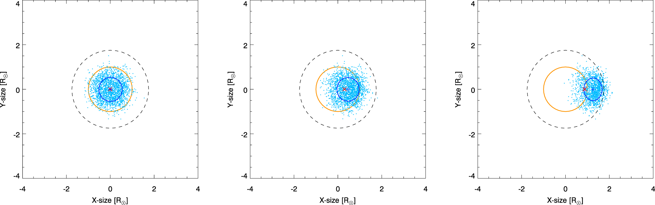
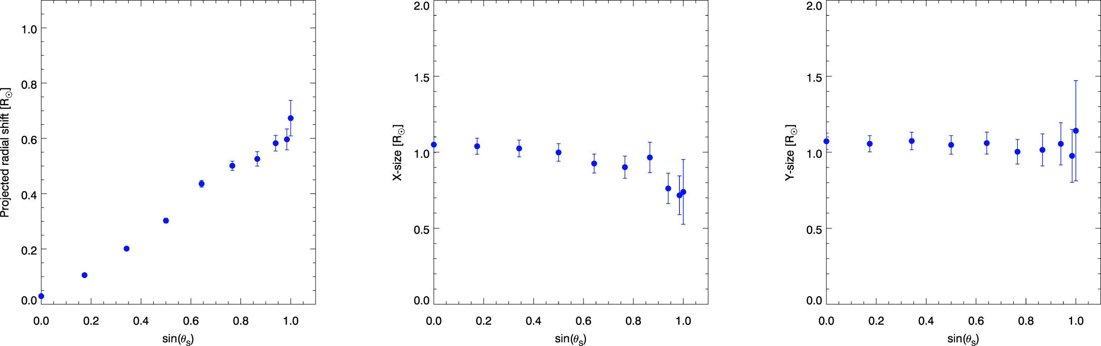
The main effects on source location and size are shown in Figure 7. Because of projection effects along the radial direction, the FWHM source size along the x-direction decreases with heliocentric angle (Figure 8), while the FWHM in the y-direction (perpendicular to the radial direction) changes only weakly, remaining 1–1.2 R_⊙. Sources located away from the disk center are shifted radially (along the x-direction in our simulations), and the near-linear dependence of the source position on sin θ_s can be clearly seen from Figure 8. The observer sees an apparent position that is shifted radially away from the disk center, with the shift projected onto the skyplane proportional to sin θ_s. While sources near the disk center θ_s = 0 are radially shifted toward the observer, the true and apparent sources coincide in the (x, y) plane of the sky. The case of more isotropic scattering (Figure 9) suggests that the degree of anisotropy only weakly affects source sizes and positions close to the disk center, but has a stronger effect close to the limb. Thus, the radial size (along the X-axis) for α = 0.5 (nearly isotropic scattering) does not decrease toward the limb as fast as in the case with stronger anisotropy α = 0.3 (Figure 8). This is consistent with the observations of angular broadening of the Crab Nebula (e.g., Dennison & Blesing 1972) by coronal turbulence, which show a preferential elongation along the tangential direction.

Zoom In Zoom Out Reset image size

Zoom In Zoom Out Reset image size

Zoom In Zoom Out Reset image size

Similarly, the interplay between scattering and the focusing effects determine the directivity of the escaping emission. The simulated directivity patterns show that although radio-wave scattering effects lead to large source sizes, the directivity (right panel in Figures 3–4) is predominately in the radial direction with half widths at half maximum ≃47° and ≃40° for anisotropy α = 0.5 and α = 0.3 correspondingly. These results are different from early results suggesting isotropic directivity due to scattering as reviewed by McLean & Melrose (1985).

It is instructive to review observations of solar radio burst source sizes and decay times for comparison with the ray-tracing results. Solar radio bursts are observed over a wide range of frequencies from about ∼500 MHz down to ∼20 kHz near 1 au. Therefore, the variation of burst parameters with frequency allows us to diagnose the scattering over a wide range of heliocentric distances.

Figure 10 combines measurements¹² by several different authors (Bougeret et al. 1970; Abranin et al. 1976; Alvarez 1976; Abranin et al. 1978; Chen & Shawhan 1978; Dulk & Suzuki 1980; Steinberg et al. 1985; Saint-Hilaire et al. 2013; Krupar et al. 2014; Kontar et al. 2017) over the last 50 years. The Type III source sizes (FWHM; degrees) are for frequencies ranging from ∼0.05 to 500 MHz. Using a weighted linear fit in log-space, the FWHM depends on the observing frequency (f; MHz) as (see Figure 10)

$$\begin{eqnarray}&&\mathrm{FWHM}=(11.8\pm 0.06)\times {f}^{-0.98\pm 0.05}.\end{eqnarray} \tag{ 50 }$$

Zoom In Zoom Out Reset image size

Similarly, a collection of Type III burst decay time measurements (Alexander et al. 1969; Aubier & Boischot 1972; Elgaroy & Lyngstad 1972; Alvarez & Haddock 1973; Barrow & Achong 1975; Krupar et al. 2018; Reid & Kontar 2018), over the frequency range from ∼0.1 to 100 MHz, is presented in Figure 10. The best-fit power-law dependence of the decay time τ (s) on frequency f (MHz) is

$$\begin{eqnarray}&&\tau =(72.2\pm 0.3)\times {f}^{-0.97\pm 0.03}.\end{eqnarray} \tag{ 51 }$$

For comparison, Wild (1950) derived an expression τ = 100 × f⁻¹ for the decay time, based on observations in the frequency range 80–120 MHz, while Alvarez & Haddock (1973) obtained τ = 51.29 × f^−0.95 based on observations in the frequency range 50 kHz–3.5 MHz, and Evans et al. (1973) obtained τ = (2.0 ± 1.2) × 100 × f^{−(1.09±0.05)} based on observations in the frequency range 67 kHz–2.8 MHz for 1/e decay.

Figure 11 shows the results of our simulations, assuming isotropic scattering. The decay time agrees within a factor of 2 with that by Krupar et al. (2018); this difference is likely due to the different numerical schemes used (see the discussion around Equation (20)). While a detailed comparison for various anisotropies would require substantial computation effort outside the scope of this work, it is nevertheless clear that isotropic scattering cannot explain the observations. For example, if the level of density fluctuations is chosen to explain the decay times, the predicted source sizes are far too small to explain the observations. Similarly, if the level of isotropic density fluctuations is chosen to match the source sizes, the decay times are too long. Evidently, anisotropic scattering, with a reduced level of scattering along the radial direction, is needed to account for both observed source sizes and decay times.

Zoom In Zoom Out Reset image size

Radio emission from solar sources is strongly affected by scattering on small-scale density fluctuations. In general, the observed source sizes and positions, time profiles, and directivity patterns are determined mainly by propagation effects and not by intrinsic properties of the primary source. We have constructed a new model that allows quantitative analysis of radio-wave propagation in a medium that contains an axially symmetric, but anisotropic, scattering component. We have compared the results of numerical simulations using this model with observations of source sizes and time profiles over a wide range of frequencies. Since plasma emission sources with small intrinsic size are observed in type III bursts (Kontar et al. 2017; Sharykin et al. 2018), the observed radio sources are dominated by the scattering, at least at these frequencies. Hence their sizes can be used as diagnostics of radio-wave propagation effects.

In general, a typical source of plasma emission (e.g., Type I, II, III, IV, or V solar radio bursts) might have a finite size FWHM_source defined by the intrinsic size of the region producing the radio emission. The observed FWHM size for such a source is given by (FWHM_source² + FWHM_scat²)^1/2, where FWHM_scat is calculated in this paper. Thus for frequencies around 35 MHz, FWHM_scat ≃ 1.1 R_⊙, so if the source is substantially smaller than this value, the observed source sizes are dominated by scattering effects. For large sources ≳1.1 R_⊙ (i.e., ≳18'), the source sizes due to scattering calculated in this paper can be subtracted in quadrature from the observed source size to give the dimensions of the intrinsic source, corrected for wave propagation effects. However, the size of density fluctuations, and hence the scattering efficiency, can vary appreciably from event to event and from one solar atmosphere region to another, consistent with the considerable variability of the density fluctuation spectrum observed in the solar wind (e.g., Celnikier et al. 1983; Marsch & Tu 1990).

The main result of our work comes from the comparison of the simulation results with combined imaging and time-delay observations. For a given density fluctuation magnitude and outer and inner scales l_o, l_i, changing the anisotropy parameter α only weakly affects the source size over a broad range of angles near the disk center. (These effects are most noticeable close to the limb, where the anisotropy direction corresponds to the line of sight.) However, the time profiles (or, equivalently, the radio pulse expansion along the line of sight) are strongly affected by the value of α. Comparison of the simulation results with observations of source size and time delay, both as a function of frequency, suggests that anisotropic density turbulence, with preferential scattering perpendicular to the solar radial direction (α ≃ 0.3) is required to account for both the source size and time-delay variations at frequencies close to 30 MHz. In order to explain the Type III observations in the heliosphere between 0.1 and 1 MHz, additional simulations are required. Indeed, the simulations by Krupar et al. (2018) demonstrate that although isotropic scattering with  ≃ 0.06–0.07, l_o and l_i given by Equation (49) can explain the decay time, the anisotropy of density fluctuations is inadequate to explain the typical source sizes (e.g., Figure 11). The numerical model developed in Section 3 suggests that the anisotropic density fluctuations (lower power in the parallel direction) are required to account for the source sizes and decay times simultaneously. This result requires further computationally intensive investigations using the method outlined in the paper.

The other interesting result is that the directivity of solar radio bursts is determined by a combination of wave focusing due to large-scale refraction and scattering on small-scale density fluctuations. At the same time, the intrinsic directivity of the source, e.g., the dipole pattern associated with radio emission near the plasma frequency (Zheleznyakov & Zaitsev 1970) is quickly lost due to scattering and thus is not evident in observations. Contrary to the results of early simulations (e.g., McLean & Melrose 1985, for a review), the resulting directivity appears to have a width of approximately 40° near 30 MHz. The observed directivity pattern is a combination of the focusing due to large-scale refraction and the scattering. The anisotropy of the density fluctuation spectrum plays an important role in governing the emission pattern of solar radio bursts. Therefore, efficient isotropization of radio waves near the emission source does not automatically imply an isotropic emission pattern as sometimes assumed.

Free–free absorption appears to have a small or negligible effect for frequencies below 30–50 MHz. However, the collisions are important for higher frequencies and can determine the time profile. It is also important to note that the stronger the scattering of radio waves, the more pronounced the effect of the free–free absorption. Photons that are strongly scattered are also absorbed stronger and hence produce a weaker contribution to the observed properties.

The effect of radio-wave scattering depends on the radial profiles of the quantities $(\bar{q}{\epsilon }^{2})(r)$ and α (r), representing the size and anisotropy of density fluctuations, respectively. For a decreasing spectrum of electron density fluctuations S(q) ∝ q^−5/3, scattering is most sensitive to the largest q (i.e., the smallest scales) in the inertial range spectrum—the scale of energy dissipation—and so provides key diagnostics for the inner scale l_i(r) (Equation (49)). At the same time, conclusions regarding the level of density fluctuations are also dependent on, and so require knowledge of, the outer density scales l₀. For example, to explain the observations near 30 MHz, a high level of density fluctuations  = 0.8 is required for the model of l_o (r) adopted, and it is possible that the model l_o(r) is not valid at these frequencies. Comparison between observations and simulations therefore provides a powerful tool with which to infer the radial variation of density fluctuations from the Sun to the Earth, which will be the subject of further work.

E.P.K. and N.L.S.J. acknowledge the financial support from the STFC Consolidated Grant ST/P000533/1. A.G.E. was supported by grant NNX17AI16G from NASA's Heliophysics Supporting Research program. V.K. acknowledges support by an appointment to the NASA postdoctoral program at the NASA Goddard Space Flight Center administered by Universities Space Research Association under contract with NASA and the Czech Science Foundation grant 17-06818Y. We also acknowledge support from the International Space Science Institute for the LOFAR http://www.issibern.ch/teams/lofar/ and solar flare http://www.issibern.ch/teams/solflareconnectsolenerg/ teams.

For isotropic density fluctuations, due to spherical symmetry,

$$\begin{eqnarray*}&&{D}_{{ij}}={D}_{0}\left({\delta }_{{ij}}-\displaystyle \frac{{k}_{i}{k}_{j}}{{k}^{2}}\right).\end{eqnarray*}$$

Taking the projection of D_ij with δ_ij gives

$$\begin{eqnarray*}&&{D}_{{ij}}{\delta }_{{ij}}={D}_{0}\left({\delta }_{{ii}}-\displaystyle \frac{{k}_{i}{k}_{i}}{{k}^{2}}\right)=2{D}_{0},\end{eqnarray*}$$

where the k_i are components of ${\boldsymbol{k}}$ and the summation over repeated indices is implicit. Using the wavenumber diffusion tensor given by Equation (7),

$$\begin{eqnarray}&&{D}_{{ij}}=\displaystyle \frac{\pi {\omega }_{{pe}}^{4}}{4\omega {c}^{2}}\int {q}_{i}\,{q}_{j}\,S(q)\,\delta ({\boldsymbol{q}}\cdot {\boldsymbol{k}})\displaystyle \frac{{d}^{3}q}{{\left(2\pi \right)}^{3}},\end{eqnarray} \tag{ 52 }$$

or, in polar coordinates,

$$\begin{eqnarray*}\begin{array}{rcl}{D}_{0} & = & \displaystyle \frac{1}{2}\displaystyle \int {q}^{2}\,S(q)\,\delta ({qk}\cos \theta )\,2\pi {q}^{2}\,d\cos \theta \,{dq}\\ & = & \ \displaystyle \frac{\pi }{k}{\displaystyle \int }_{0}^{\infty }{q}^{3}\,S(q)\,{dq}.\end{array}\end{eqnarray*}$$

Hence one finds that Equation (52) can be written as

$$\begin{eqnarray}&&{D}_{{ij}}=\left({\delta }_{{ij}}-\displaystyle \frac{{k}_{i}{k}_{j}}{{k}^{2}}\right)\displaystyle \frac{1}{32\pi }\displaystyle \frac{{\omega }_{{pe}}^{4}}{\omega {c}^{2}k}{\int }_{0}^{\infty }{q}^{3}\,S(q)\,{dq}.\end{eqnarray} \tag{ 53 }$$

This wave vector diffusion tensor has the same structure as that for Langmuir waves (e.g., Goldman & Dubois 1982; Muschietti & Dum 1991; Ratcliffe et al. 2012).

Following early works by Hollweg (1970) and Steinberg et al. (1971) we assume that the density fluctuations have a Gaussian correlation, so the Gaussian autocorrelation function of the density fluctuations is

$$\begin{eqnarray}&&C(r)=\displaystyle \frac{\langle n(0)\,n({\boldsymbol{r}})\rangle }{{n}^{2}}=\displaystyle \frac{\langle \delta {n}^{2}\rangle }{{n}^{2}}\exp \left(-\displaystyle \frac{{r}_{\perp }^{2}}{{h}_{\perp }^{2}}-\displaystyle \frac{{r}_{\parallel }^{2}}{{h}_{\parallel }^{2}}\right),\end{eqnarray} \tag{ 54 }$$

where ${h}_{\perp }^{2}$ and h_∥ are the perpendicular and parallel correlation lengths, respectively, and $\langle \delta {n}^{2}\rangle$ is the variance of density fluctuations. For isotropic fluctuations,

$$\begin{eqnarray}&&C(r)=\displaystyle \frac{\langle n(0)\,n({\boldsymbol{r}})\rangle }{\langle n{\rangle }^{2}}=\displaystyle \frac{\langle \delta {n}^{2}\rangle }{{n}^{2}}\exp \left(-\displaystyle \frac{{r}^{2}}{{h}^{2}}\right),\end{eqnarray} \tag{ 55 }$$

where h = h_⊥ = h_∥ is the correlation length. The spectrum S(q), defined as

$$\begin{eqnarray*}&&S(q)=\int C(r){e}^{-i{\boldsymbol{k}}\cdot {\boldsymbol{r}}}\,{d}^{3}r,\end{eqnarray*}$$

also has a Gaussian form

$$\begin{eqnarray}&&S(q)=\displaystyle \frac{\langle \delta {n}^{2}\rangle }{{n}^{2}}\,{\left(\pi {h}^{2}\right)}^{3/2}\exp \left(-\displaystyle \frac{{q}^{2}{h}^{2}}{4}\right),\end{eqnarray} \tag{ 56 }$$

so that the variance of density fluctuations is

$$\begin{eqnarray}&&\displaystyle \frac{\langle \delta {n}^{2}\rangle }{{n}^{2}}={\epsilon }^{2}=\int S(q)\,\displaystyle \frac{{d}^{3}q}{{\left(2\pi \right)}^{3}}={\int }_{0}^{\infty }S(q)\,4\pi {q}^{2}\,\displaystyle \frac{{dq}}{{\left(2\pi \right)}^{3}}.\end{eqnarray} \tag{ 57 }$$

Substituting the isotropic Gaussian spectrum (56) into the wave vector diffusion tensor (53), one finds

$$\begin{eqnarray*}\begin{array}{rcl}{D}_{{ij}} & = & \left({\delta }_{{ij}}-\displaystyle \frac{{k}_{i}{k}_{j}}{{k}^{2}}\right)\displaystyle \frac{1}{32\pi }\,\displaystyle \frac{{\omega }_{{pe}}^{4}}{\omega {c}^{2}k}{\displaystyle \int }_{0}^{\infty }{q}^{3}\,S(q)\,{dq}\\ & = & \ \left({\delta }_{{ij}}-\displaystyle \frac{{k}_{i}{k}_{j}}{{k}^{2}}\right)\displaystyle \frac{\sqrt{\pi }}{4}\displaystyle \frac{\langle \delta {n}^{2}\rangle }{{{hn}}^{2}}\displaystyle \frac{{\omega }_{{pe}}^{4}}{\omega {c}^{2}k}.\end{array}\end{eqnarray*}$$

The average wavenumber vector q, given by Equation (8), for the density fluctuation spectrum of Equation (56), is

$$\begin{eqnarray}\begin{array}{rcl}\bar{q} & = & \displaystyle \frac{1}{{\epsilon }^{2}}\displaystyle \int q\,S(q)\,\displaystyle \frac{{d}^{3}q}{{\left(2\pi \right)}^{3}}={\left(\pi {h}^{2}\right)}^{3/2}{\displaystyle \int }_{0}^{\infty }{q}^{3}\\ & & \times \ \exp \left(-\displaystyle \frac{{q}^{2}{h}^{2}}{4}\right)\,\displaystyle \frac{{dq}}{{\left(2\pi \right)}^{3}}=\displaystyle \frac{4}{\sqrt{\pi }h},\end{array}\end{eqnarray} \tag{ 58 }$$

so that the diffusion coefficient D_θθ becomes

$$\begin{eqnarray}\begin{array}{rcl}{D}_{\theta \theta } & = & \displaystyle \frac{{\pi }^{2}}{4}\displaystyle \frac{{\omega }_{{pe}}^{4}}{\omega {c}^{2}{k}^{3}}\,\displaystyle \frac{1}{{\left(2\pi \right)}^{3}}{\displaystyle \int }_{0}^{\infty }{q}^{3}\,S(q)\,{dq}\\ & = & \displaystyle \frac{\sqrt{\pi }}{4h}\,\displaystyle \frac{\langle \delta {n}^{2}\rangle }{{n}^{2}}\,\displaystyle \frac{{\omega }_{{pe}}^{4}}{{c}^{2}\omega {k}^{3}}\\ & = & \ \displaystyle \frac{\pi }{16}\,\bar{q}\,{\epsilon }^{2}\displaystyle \frac{{\omega }_{{pe}}^{4}}{{c}^{2}\omega {k}^{3}},\end{array}\end{eqnarray} \tag{ 59 }$$

where ${\epsilon }^{2}=\langle \delta {n}^{2}\rangle /{n}^{2}$. The angular scattering rate per unit time becomes

$$\begin{eqnarray}&&\displaystyle \frac{d\langle {\theta }^{2}\rangle }{{dt}}=2{D}_{\theta \theta }=\displaystyle \frac{\pi }{8}\,\bar{q}\,{\epsilon }^{2}\,\displaystyle \frac{{\omega }_{{pe}}^{4}}{{c}^{2}\omega {k}^{3}}\end{eqnarray} \tag{ 60 }$$

or, per unit distance, for a photon with group speed v_gr = c²k/ω,

$$\begin{eqnarray}\begin{array}{rcl}\displaystyle \frac{d\langle {\theta }^{2}\rangle }{{dx}} & = & \displaystyle \frac{1}{{v}_{{gr}}}\,\displaystyle \frac{d\langle {\theta }^{2}\rangle }{{dt}}=\displaystyle \frac{\pi }{8}\,\bar{q}\,{\epsilon }^{2}\,\displaystyle \frac{{\omega }_{{pe}}^{4}}{{c}^{4}\,{k}^{4}}\\ & = & \displaystyle \frac{\pi }{8}\,\bar{q}\,{\epsilon }^{2}\displaystyle \frac{{\omega }_{{pe}}^{4}}{{\left({\omega }^{2}-{\omega }_{{pe}}^{2}\right)}^{2}}\\ & = & \ \displaystyle \frac{\sqrt{\pi }}{2}\,\displaystyle \frac{{\epsilon }^{2}}{h}\,\displaystyle \frac{{\omega }_{{pe}}^{4}}{{\left({\omega }^{2}-{\omega }_{{pe}}^{2}\right)}^{2}},\end{array}\end{eqnarray} \tag{ 61 }$$

an expression widely used (e.g., Chandrasekhar 1952; Hollweg 1968, 1970; Steinberg et al. 1971; Lacombe et al. 1997; Chrysaphi et al. 2018; Krupar et al. 2018; Gordovskyy et al. 2019) and identical to the expression (27) in Arzner & Magun (1999) (noting that $h=\sqrt{2}l$ needs to be redefined to obtain $2{\eta }^{* }=d\langle {\theta }^{2}\rangle /{dt}$).

In situ observations of density fluctuations suggest an inverse power-law spectrum of density fluctuations S(q) ∝ q^−(p + 2), with the exponent p close to 5/3 as observed (Alexandrova et al. 2013). This power-law normally holds over a broad inertial range from outer scales l₀ = 2π/q₀ to inner scales l_i = 2π/q_i (see, e.g., Alexandrova et al. 2013, for a review):

$$\begin{eqnarray}S(q)=\left\{\begin{array}{ll}0, & q\gt {q}_{0}\\ {\rm{const}}\times {q}^{-(p+2)}, & {q}_{i}\lt q\lt {q}_{0},\\ 0, & q\lt {q}_{i}\end{array}\right.\end{eqnarray} \tag{ 62 }$$

where the constant follows by normalizing the integrated spectrum to the level of density fluctuations $\langle \delta {n}^{2}\rangle$. Then the spectrum-weighted average wavenumber $\bar{q}$ (Equation (8)) becomes (Lacombe et al. 1997; Arzner & Magun 1999)

$$\begin{eqnarray}&&\bar{q}=\displaystyle \frac{(p-1)}{(p-2)}\,\displaystyle \frac{{q}_{i}^{2-p}-{q}_{0}^{2-p}}{{q}_{i}^{1-p}-{q}_{0}^{1-p}}.\end{eqnarray} \tag{ 63 }$$

This is often simplified further by assuming a large range of wave numbers, so that q_o ≪ q_i. For example, Thejappa et al. (2007) and Krupar et al. (2018) used Equation (63) with p = 5/3 in the limit q_o ≪ q_i, giving the particularly simple form

$$\begin{eqnarray}&&\bar{q}\simeq 2\,{q}_{0}^{2/3}{q}_{i}^{1/3}=4\pi {l}_{0}^{-2/3}{l}_{i}^{-1/3},\end{eqnarray} \tag{ 64 }$$

for which the variance of density fluctuations is

$$\begin{eqnarray}&&{\epsilon }^{2}=\int S(q)\,\displaystyle \frac{{d}^{3}q}{{\left(2\pi \right)}^{3}}={\int }_{0}^{\infty }S(q)\,4\pi {q}^{2}\,\displaystyle \frac{{dq}}{{\left(2\pi \right)}^{3}}.\end{eqnarray} \tag{ 65 }$$

Then the scattering rate with $\bar{q}$ given by (64) becomes

$$\begin{eqnarray}\begin{array}{rcl}\displaystyle \frac{d\langle {\theta }^{2}\rangle }{{dt}} & = & 2\displaystyle \frac{\pi }{16}\,\bar{q}\,{\epsilon }^{2}\displaystyle \frac{{\omega }_{{pe}}^{4}}{{c}^{2}\omega {k}^{3}}=\displaystyle \frac{{\pi }^{2}}{4}{l}_{0}^{-2/3}{l}_{i}^{-1/3}{\epsilon }^{2}\displaystyle \frac{{\omega }_{{pe}}^{4}}{{c}^{2}\omega {k}^{3}}\\ & = & \ \displaystyle \frac{{\pi }^{2}}{2}{l}_{0}^{-2/3}{l}_{i}^{-1/3}{\epsilon }^{2}\displaystyle \frac{{\omega }_{{pe}}^{4}c}{\omega {\left({\omega }^{2}-{\omega }_{{pe}}^{2}\right)}^{3/2}}.\end{array}\end{eqnarray} \tag{ 66 }$$

Expressed as a scattering per unit of length x, Equation (66) is

$$\begin{eqnarray}&&\displaystyle \frac{d\langle {\theta }^{2}\rangle }{{dx}}=\displaystyle \frac{{\pi }^{2}}{2}{l}_{0}^{-2/3}{l}_{i}^{-1/3}{\epsilon }^{2}\displaystyle \frac{{\omega }_{{pe}}^{4}}{{\left({\omega }^{2}-{\omega }_{{pe}}^{2}\right)}^{2}}.\end{eqnarray} \tag{ 67 }$$

This is the expression used by Thejappa & MacDowall (2008) and Krupar et al. (2018), but includes an additional factor of π/2. It also coincides with Equation (30) from Arzner & Magun (1999).