


Abstract
Magnetosheath properties, particularly those related to magnetopause magnetic reconnection (MR), are investigated in this study. (1) Asymmetries are found to exist in the distributions of plasma and magnetic field parameters in the magnetosheath. These asymmetries are related to the interplanetary magnetic field (IMF) orientation, and they are produced either on the bow shock or inside the magnetosheath. Thus, one must be very cautious in directly using the upstream solar wind and IMF properties as the magnetopause MR initiation conditions, since the magnetosheath parameters are not the same everywhere. (2) A unique method is introduced to estimate how much IMF magnetic flux passes through the magnetosphere via MR on either the low-latitude or the high-latitude magnetopause. This flux mainly varies with three independent parameters: the IMF clock angle θCL, the magnetosheath plasma β, and the solar wind sound Mach number MS. Surprisingly, the magnetic fluxes passing through the magnetosphere are comparable under the southward and northward IMF conditions. (3) The dipole tilt angle, the property from the inside of the magnetosphere, also controls the magnetosheath parameters. As the Earth's dipole tilt angle varies, the plasma pressure ridge shifts its location but remains near the magnetic equator. The stagnation point of the magnetosheath flow on the magnetopause, however, remains at the subsolar point no matter how large the dipole tilt angle is. These behaviors may be determinative of the locations of MR and the generation of flux transfer events on the magnetopause.
Export citation and abstract BibTeX RIS
1. Introduction
When the supersonic solar wind impacts the Earth's magnetosphere, a transition region, the magnetosheath, forms ahead of the magnetosphere. The bow shock is the outermost boundary of this transition region, where the magnetized solar wind goes through dramatic changes in plasma density, velocity, pressure, and field strength and orientation. Behind the bow shock, the shocked plasma, carrying the bent interplanetary magnetic field (IMF), continues to be compressed and diverted when heading toward the magnetopause, the innermost boundary of the transition region. At the magnetopause, the plasma stops or flows along the magnetopause. The shocked solar wind finally returns to the downstream solar wind or enters the magnetosphere through the transport processes on the magnetopause, such as magnetic reconnection (MR), the Kelvin–Helmholtz instabilities, or other diffusion processes. The properties of the magnetosheath, particularly those adjacent to the magnetopause, are crucial to the initiation and proceeding of these transport processes.
A transport phenomenon frequently seen on the magnetopause, MR allows the mass, moment, and energy exchange across the magnetopause. It is usually described as a development of the tearing mode instability in a current sheet embedded within a highly conducting plasma. This is, however, a convenient approximate magnetohydrodynamic (MHD) description for actual situations by invoking a suitable ad hoc "anomalous resistivity" and separating the MR physics from the question of what mechanisms cause the dissipation enabling MR (Priest 1985). This question, however, should be answered in a kinetic regime (Pritchett 2015). The recently launched Magnetospheric Multiscale satellites (MMS) provide observations inside or near diffusion regions of MR in space with higher temporal and special resolution at electron scales, which makes a great opportunity to explore the kinetic processes enabling MR (Burch et al. 2016). A lot of progress has been made in understanding the kinetic aspects of MR initiation, including the plasma wave and turbulence (Cao et al. 2017; Ergun et al. 2017; Graham et al. 2018; Munoz & Buchner 2018), the Hall physics (Alm et al. 2018), and the electron dynamics (Torbert et al. 2016; Egedal et al. 2018; Genestreti et al. 2018; Wang et al. 2018). All of these observations regarding the general Ohm's law have greatly enriched the community's knowledge of MR, although sometimes it is difficult to assert whether a specific phenomenon is the result or the cause of MR. Specific to the magnetopause MR, the aforementioned question is equivalent to another question of where MR prefers to occur. It is generally thought that MR distributes along a belt on the magnetopause, which is referred to as an X line. It is reasonable to believe that these loci may have some extreme properties, since MR occurs there but does not occur elsewhere, and thus it is most likely to investigate the triggering processes or initiation conditions at those loci.
A variety of models have been established to predict the location and extension of an X line on the magnetopause by seeking the extreme quantities of some parameters over the magnetopause (Komar et al. 2015), and all of these parameters are shown to depend strongly on the magnetosheath properties adjacent to the magnetopause. Electric current is a key factor in these models, since the tearing mode instability is a current-driven instability (Priest 1985). An early current-based model proposes that magnetopause MR prefers to occur where the geomagnetic field and the IMF are antiparallel (antiparallel MR; Crooker 1979; Luhmann et al. 1984). The antiparallel MR loci typically line up at high latitudes when the IMF has a finite BY component (Trattner et al. 2007) and at low latitudes if the IMF is nearly southward (Moore et al. 2002). Subsequent investigations reveal, however, that MR can occur where the fields are not purely antiparallel (component MR; Sonnerup 1974; Cooling et al. 2001; Moore et al. 2002; Pu et al. 2005; Trattner et al. 2007), and MR thus involves a pair of antiparallel reconnecting components and a pair of out-of-plane guide field components. By invoking a constraint that the pair of guide fields should be of the same magnitude, Gonzalez & Mozer (1974) and Sonnerup (1974) developed a current-based component MR model and proposed that MR loci should spread along the local current directions (the guide field directions). This constraint, however, cannot specify the location of an X line on the magnetopause unless at least one reconnecting locus on the X line is already known (Cooling et al. 2001). An additional constraint was thus imposed that MR is excited where the local current density is great enough to cause the anomalous resistivity (Pudovkin & Semenov 1985; Alexeev et al. 1998). After the initiation, MR may spread or extend out of the reconnecting plane at the speed of the local current or the out-of-plane Alfvén speed (Shay et al. 2003; Katz et al. 2010; Walsh et al. 2018). There are also other MR models that are not established on the basis of the electric current. For example, by invoking an alternative constraint into the component MR model that the reconnecting components should be of equal magnitude, a non-current-based model predicts that an X line anchors at the locus of the largest reconnecting field magnitude and extends along the local guide field directions, which are not necessarily along the current directions (Moore et al. 2002). Trattner et al. (2007) developed a geometry-based model and assumed that an X line consists of the points of the maximum shear angles θX on the single sheath field lines wrapped around the dayside magnetopause (shear angle ridge). The magnetic shear angle θX is the angle between the magnetosheath magnetic field and the geomagnetic field beside the magnetopause. Clearly, no matter whether it is for the current- or non-current-based MR models, knowledge of the magnetosheath properties over the whole magnetopause is critical for seeking the extreme conditions that allow the initiation of MR on the magnetopause.
Where MR occurs on the magnetopause remains under debate (Souza et al. 2017). It suffers from the insufficiency of the satellite observations to examine the aforementioned MR location models. One major difficulty is subject to looking for the extremum conditions throughout the whole dayside magnetopause. From the observation point of view, neither single nor multiple satellite observations can provide enough information to retrieve the maxima or minima of a parameter over the whole magnetopause. Another difficulty is that it is hard to determine the MR locations by using satellite observations if one wants to compare them with the modeled ones. The best way to confirm that MR is ongoing right at the site of an observing satellite is to let the satellite traverse the MR structure in the direction tangential to the magnetopause, and the oppositely directed jet flows from the MR site, the reversed magnetic field components normal to the local magnetopause, or even the Hall effect inside the MR structure can be the features indicative of the MR occurrence. It turns out, however, that it is rare to have a satellite to traverse an X line on the magnetopause (Phan et al. 2000). It is probably because a satellite usually traverses the magnetopause fast and cannot stay around the magnetopause for long, and thus it has little chance to encounter an X line. Fortunately, the energy dispersion of the particles ejected from an X line can be used to infer the initiation locations of MR even though the observing satellite is far away from the X line (Trattner et al. 2007; Zhu et al. 2015). Both the case studies and the statistics of Zhu et al. (2015) reveal that X lines tend to shift away from the subsolar region, southward or northward, depending on how the dipole axis of the Earth rotates. The dipole tilt angle θd is the quantity to describe the rotation of the Earth's dipole axis, and it is a key factor from the inside of the magnetosphere to affect the shape and size of both the magnetopause and the bow shock (Lu et al. 2011; Liu et al. 2012). Further investigation is desired to answer the question of what role the dipole axis plays in shifting MR or X lines on the magnetopause.
How fast MR goes, i.e., the MR rate, is another key problem. This rate is usually quantified by a local reconnecting electric field ER = BRVin, where BR is the reconnecting magnetic field component and Vin is the plasma velocity in the inflow region toward MR. This quantity describes how much magnetic flux rushes into the MR diffusion region and is reconnected per unit time and unit length along the X line (Sonnerup 1974). Here ER is a very localized parameter, and its quantity is closely related to the local inflow parameters, such as the field magnitudes and orientations and the plasma density (Sonnerup 1974; Cassak & Shay 2007; Liu et al. 2018). For example, by using a simple two-dimensional MR model with an incompressible plasma, Sonnerup (1974) demonstrated that the magnetic shear angle θX, the reconnecting field magnitudes BR, and the local Alfvén speed VA,in (a function of the reconnecting field BR and the local plasma density ρ) in the inflow region all control ER: the larger shear angle θX the fast MR; for a given θX, a weak enough sheath magnetic field may prevent MR from happening and MR goes faster when the sheath field increases. The flow speed toward the X line Vin, which carries the magnetic flux into the MR diffusion region, is thought to be a fraction of the local Alfvén speed Vin = kVA,in, where k is an unchanged coefficient. If ER is normalized by the local inflow parameters BR and VA,in as  , the dimensionless quantity
  is in fact equal to k. Under a two-dimensional MHD constraint, Liu et al. (2018) revealed that this dimensionless quantity
  or k also depends on the inflow field magnitudes BR and plasma densities ρ and may range from 0.1 to 10, but for the typical magnetopause case, it remains about 0.1, i.e., ER ≈ 0.1BRVA,in.
The theoretical results of Sonnerup (1974) have in fact hinted that the plasma β (the ratio of the pressures of the plasma and the magnetic field) acts on the MR rate ER, since both ER and β are determined by the field magnitude BR and the plasma densities ρ in the MR inflow region. Sonnerup (1974) showed that a smaller plasma β in the sheath means a faster MR on the magnetopause and that MR may cease when β is big enough. Phan et al. (2013) studied the dependence of the MR occurrence on both the plasma β and the magnetic shear θX, and they found that a small β difference beside the magnetopause allows MR to occur over a large range of magnetic shears, whereas when the difference is big, MR occurs only for the high magnetic shears. Since the plasma β is typically much lower in the magnetosphere than that in the magnetosheath, the difference in β beside the magnetopause is in fact dominated by the sheath plasma β. In this sense, the results of Phan et al. (2013) are consistent with those of Sonnerup (1974). Swisdak et al. (2003) attributed the forbiddance of MR to the fast diamagnetic drift of an X line, and MR stops when the sheath plasma β is as high as the corresponding diamagnetic drift velocity exceeds the local Alfvén velocity. The local Alfvén velocity is thus the other key parameter in the magnetosheath for the proceeding of MR, and a steady-state MR cannot occur unless the background sheath flow is slower than the local Alfvén velocity (sub-Alfvénic; Cowley & Owen 1989; Cooling et al. 2001).
To measure the inflow parameters from satellite observations and thus calculate the local ER or  , however, is very difficult, mainly suffering from the motion and geometry of the local magnetopause (Wang et al. 2015c). For example, the magnitude of the inflow plasma velocity, Vin, can be measured only if the normal direction of the local magnetopause and the magnetopause motion along this normal direction are known precisely; the reconnecting magnetic field component, BR, and thus the corresponding Alfvén velocity, VA,in, cannot be obtained unless the MR out-of-plane direction is already known. In this situation, the integral of ER along an X line
  , i.e., the potential drop imposed on the magnetopause by MR, is usually used to evaluate the total magnetic flux input into the magnetosphere per unit time through the magnetopause X line (Sonnerup 1974; Newell et al. 2007; Milan et al. 2012). This global reconnection rate
  , however, is still not able to be determined directly according to its definition, i.e., integrating ER along the X line, owing to a lack of knowledge of both the length of the X line and the variation of ER along the X line. In practice,
  is usually estimated through the open magnetic flux newly added into the polar cap
  (Milan et al. 2012). Then,
  is written as a function of the solar wind properties in the form of
  to explicitly describe the coupling efficiency between the solar wind and the magnetosphere, where
  is typically an IMF clock angle dependent solar wind convection electric field by using which to substitute the reconnection electric field ER and Leff is the effective width of the channel of the magnetic flux in the upstream solar wind impinging on the bow shock that is eventually reconnected at the magnetopause (Milan et al. 2012). Here
  can be
(Burton et al. 1975; Holzer & Slavin 1978), where BS is the IMF southward component, VX is the anti-sunward component of the solar wind velocity in the geocentric solar magnetospheric (GSM) coordinate system, BYZ is the projection of the IMF on the YZ plane of the GSM system, and θCL is the IMF clock angle defined as  if BY > 0 and
  if BY < 0; or

(Sonnerup 1974); or

(Wygant et al. 1983); or

(Milan et al. 2012). There are even more complicated forms for  determined by the upstream solar wind plasma density ρSW, as well as by the solar wind VX, BYZ, and θCL (Vasyliunas et al. 1982; Scurry & Russell 1991). The dependence of
  on ρSW sounds reasonable, since
  describes the average of ER, and ER depends on ρSW. The control of the solar wind plasma properties to the magnetopause MR rate may also be represented by the effective width Leff. In the literature, Leff is roughly estimated to be 0.1–0.2 of the width of the magnetosphere (Reiff et al. 1981), 5–8RE on the basis of Equation (1) (Milan 2004), 2.75RE based on Equation (2) (Milan et al. 2008), or

if  is in the form of Equation (4) (Milan et al. 2012). In Equations (4) and (5), Milan et al. (2012) actually demonstrated that ρSW does not control
  .
.
The MR rate varies even when the solar wind conditions are steady, and the magnetosheath flow pattern is thought to be another critical factor that may modify the local MR rate. The global simulations show that MR does not significantly modify the local sheath parameters, and the proceeding of MR cannot modify the MR rate or stop MR by itself (Borovsky et al. 2008). That is to say, MR should be steady and may last for a long time on the magnetopause if the outside conditions are steady. The MR rate, however, does vary with time in some circumstances, and this kind of MR is usually referred to as the transient MR. Flux transfer events (FTEs) are the magnetic flux ropes lying on and moving along the magnetopause, and since FTEs were discovered by Russell & Elphic (1978), they have been regarded as a product and thus a good representative of the transient MR on the magnetopause (Russell & Elphic 1978; Southwood et al. 1988). How MR generates an FTE remains controversial, and recently, Raeder (2006) proposed a model in which the FTEs form depending on the existence of sheath flows. In this model, when the dipole tilt angle of the Earth θd is not zero, the background magnetosheath flow present at the locus of an X line can carry the X line away from its initial location, and an FTE forms between the leaving X line and a second X line while it forms at this location. This scenario is supported by the observations provided by Zhang et al. (2012), Pu et al. (2013), and Zhong et al. (2013). The flow in this model acts to modify the local MR rate, and the pattern of the sheath flow outside the magnetopause is thus crucial to the formation of FTEs. In the literature, however, the flow pattern has not been systematically examined even in an observational sense.
The MR-generated FTEs have also been observed at different planets, e.g., the Earth, Mercury, and Jupiter. At the Earth, FTEs generally last for a time of order of a minute, while at Mercury, with a magnetosphere of a size about 1/20 of the Earth's, the durations of FTEs are typically several seconds, which is also about 1/20 of the Earth's FTEs (Russell 1995). Why their durations are related to the dimensions of the planets is an interesting question and remains unclear. At Jupiter, FTEs are observed to be weaker than expected, and at Saturn or beyond, FTEs are apparently absent (Russell 1995). Russell (1995) noticed that the solar wind parameter significantly increasing with heliocentric distance is the magnetosonic Mach number MMS, which produces the higher plasma β at the nose of the magnetopause at the outer planets. The MR rate decreases in a high β plasma, which reduces the occurrence probability or even forbids the formation of FTEs (Sonnerup 1974; Russell 1995; Swisdak et al. 2003; Phan et al. 2013).
The magnetosheath properties, especially those adjacent to the magnetopause, including the field magnitude, the magnetic shear θX, the plasma β, the plasma density ρ, and even the flow pattern, are important to the initiation and proceeding of MR. To determine these parameters, however, is difficult, although the sheath properties right behind the bow shock can be determined directly by the upstream conditions through the Rankine–Hugoniot conservation law (Margaret G. Kivelson 1995). Theoretically, four quantities in the solar wind dominate the properties of the magnetosheath just behind a bow shock; they are the polytropic index (γ), the upstream sonic Mach number (MS), the IMF orientation relative to the normal of the local bow shock (ϕBS), and the solar wind βSW. Here γ is generally thought to be a constant. The MS is the ratio of the solar wind velocity to the sound speed of the solar wind plasma, and here the solar wind velocity is typically the velocity component in the direction normal to the local bow shock. The plasma deceleration and compression strongly depend on this quantity, and a larger MS has a stronger bow shock. Another crucial factor, ϕBS, determines the type of bow shock: the bow shock is referred to as the "parallel shock" if the IMF is parallel or antiparallel to the normal of the local shock (ϕBS = 0°), the "perpendicular shock" if the IMF is perpendicular to the normal direction (ϕBS = 90°), and the "oblique shock" if the IMF orientates in between. The plasma and field quantities through the bow shock are as listed below for the parallel shock,

and for the perpendicular shock,

respectively, where ρ,  , and B denote the plasma density, velocity, and field magnitude; the subscript "SW" denotes the upstream solar wind; and the subscript "⊥" denotes the component perpendicular to the local bow shock. It is clearly seen in these equations that the compression of the magnetic field strongly depends on the IMF orientation, i.e., ϕBS: for the parallel shock, the field magnitude remains unchanged, but for the perpendicular shock, the magnetic field is compressed significantly by a factor of ∼4. The deceleration and compression of plasma depend more on MS, but when the solar wind MS is large enough, the plasma behaviors are almost the same no matter what MS and ϕBS are. Since the magnetic field and the plasma behave differently at the bow shock, the solar wind plasma βSW, which describes the relative contributions of the significance of the magnetic field and the plasma to a plasma process, is thus determinative of the total compression and deceleration effect of a bow shock.
However, the upstream solar wind and IMF conditions and the Rankine–Hugoniot relations cannot provide enough information to determine the parameters in the magnetosheath unless the positions (shape and size) of the bow shock and magnetopause are already known. For example, for a given IMF, the geometry of the bow shock determines the local ϕBS on the bow shock and thus is critical to the sheath parameters downstream of the shock. The shape and size of the magnetopause, which describe the properties of the obstacle to the incident solar wind, certainly are determinative of both the sheath properties and the bow shock position. Even in an aerodynamic situation with a rigid obstacle, only an approximate solution was proposed for the shape and size of the bow shock (Farris & Russell 1994), and the analytical solutions have never been achieved (Petrinec & Russell 1997), let alone for the magnetized plasma with an elastic magnetopause obstacle.
The shape and size of the bow shock are usually described empirically in the literature. Observations or numerical simulations have revealed that many parameters in the upstream solar wind—e.g., the dynamic pressure (Pdyn); solar wind velocity ( ); magnetosonic, sonic, and Alfvén Mach numbers (MMS, MS, and MA); plasma beta βSW; and IMF strength and orientation—all have observational effects on the bow shock positions (Fairfield 1971; Farris & Russell 1994; Cairns & Lyon 1996; Bennett et al. 1997; Chapman & Cairns 2003; Dmitriev et al. 2003; Chapman et al. 2004; Chai et al. 2014; Wang et al. 2015a; Liu et al. 2016). Empirical models have been built on the basis of these controlling factors to describe the bow shock positions. The bow shock in these models can be rotationally symmetric (Fairfield 1971; Farris & Russell 1994; Cairns & Lyon 1995; Bennett et al. 1997) or asymmetric (Chapman & Cairns 2003), but most of them are in the base form of a hyperbola, which can be written as

where

is the distance of (x, y, z) on the shock to the focus at  , ε is the eccentricity, L is the semi–latus rectum, and θBS is the angle at the focus from the major axis to (x, y, z).
The other difficulty in determining the magnetosheath properties is caused by the difficulty in obtaining the exact solution of the magnetopause position. It is well known that the simple principle to determine the position of the magnetopause is the pressure balance beside the magnetopause (Schield 1969). By using a one-dimensional aerodynamic model, the plasma thermal pressure at the flow stagnation point just outside the magnetopause is derived theoretically to be almost a constant of ∼89% of the solar wind dynamic pressure Pdyn (Margaret G. Kivelson 1995). The pressure balance between this plasma pressure and the pressure of the geomagnetic field right inside the magnetopause can be used to estimate the standoff distance of the magnetopause nose (Margaret G. Kivelson 1995). For the real case—i.e., the solar wind plasma is magnetized, the bow shock and magnetopause are not one-dimensional, and the magnetopause is elastic—the problem is not that simple because of the nonlinear interactions among them. The observations and numerical simulations have revealed that the position of the magnetopause is a function of the solar wind parameters, e.g., the IMF strength and orientation, and the solar wind dynamic pressure (Pdyn; Sibeck et al. 1991; Suvorova et al. 2010; Lu et al. 2011, 2013; Liu et al. 2015; Suvorova & Dmitriev 2015, 2016). The simulations show that the geometry of the Earth's dipole (θd) also modifies the shape of the magnetopause and induces asymmetries (Liu et al. 2012). This asymmetry even transfers upstream to the bow shock and leads to an asymmetric bow shock (Wang et al. 2015b; Lu et al. 2017). Since Fairfield (1971), many empirical magnetopause models, parameterized by the conditions of the solar wind, the IMF, and the geomagnetic field, have been developed (Shue et al. 1997; Lin et al. 2010; Zhong et al. 2014; Suvorova & Dmitriev 2015, 2016). For example, by using the low-latitude magnetopause crossing data, Shue et al. (1997) established a magnetopause model of the form as follows:
where r is the distance to the center of the Earth of a point on the magnetopause, θMP is the solar zenith angle of the point, and r0 and α are the subsolar magnetopause standoff distance and the level of tail flaring of the magnetopause, respectively. Lin et al. (2010) modified the functional form of Equation (10) and established a new model in which the dipole tilt angle θd is involved and the cusp magnetopause can be well represented.
Physical processes on the inner boundary of the magnetosheath, i.e., the magnetopause, also modify the properties of the magnetosheath. The magnetopause is generally a tangential discontinuity separating the magnetosphere and magnetosheath, and the mass, moment, and energy cannot exchange across the boundary if no diffusion processes on the magnetopause occur. When the magnetic shear θX is low, a magnetosheath transition layer, also called the "plasma depletion layer," forms in front of the magnetopause (Phan et al. 1994). In this situation, when the shocked solar wind rushes toward the magnetopause, the magnetosheath magnetic field piles up against the magnetopause, and the compressed magnetic field squeezes the plasma out of the flux pileup region (Zwan & Wolf 1976), which makes the plasma density, temperature, and plasma β in this region lower and the field magnitude stronger than the quantities in the magnetosheath ahead (Phan et al. 1994). If the magnetic shear θX is high, however, the plasma depletion layer disappears, the magnetic flux does not pile up, and there are no systematic variations in the plasma parameters when approaching the magnetopause from the sheath side (Phan et al. 1994). In this situation, MR plays a significant role, and less impediment of the magnetopause prevents the formation of the depletion layer. The erosion of the magnetosphere due to MR also makes the inward motion of the magnetopause (Aubry et al. 1970; Phan et al. 1996), and, in turn, the relocation or reshaping of the magnetopause, i.e., the resizing of the obstacle, can certainly result in secondary changes in the magnetosheath properties.
In practice, due to the difficulties in obtaining the overall properties of the sheath, one may roughly use the single solar wind and IMF conditions observed outside the bow shock to represent the initiation conditions for MR, for example, using the IMF clock angle θCL to represent the magnetic shear angle θX on the magnetopause. This simplification clearly has ignored the modification of the magnetosheath to the solar wind and IMF (Cooling et al. 2001), and for a given IMF θCL, the magnetic shear θX can be very different at the different locations on the magnetopause. From the very early years, great efforts have been exerted in establishing a variety of numerical models for the overall sheath properties (Spreiter et al. 1966; Hundhaus et al. 1969; Kobel & Fluckiger 1994; Romashets et al. 2008; Nabert et al. 2013), and few of these models self-consistently describe the locations of the bow shock, the magnetopause, and the processes ongoing in the magnetopause. For example, using a high-β MHD model, Spreiter et al. (1966) provided analytical solutions for the sheath plasma and field parameters and found that the draping magnetic field presents asymmetries on the magnetopause when the cone angle θCO of the IMF is not zero ( , where BX, BY, and BZ are the three IMF components in GSM). In this situation, one cannot use a single IMF to represent the field properties outside the magnetopause. Hundhaus et al. (1969) examined the flow pattern over the magnetosheath and found that the geometry of the dipole axis cannot produce any asymmetry on the sheath flow distribution. The statistics or distributions of the satellite observations over the whole magnetosheath may be a feasible way to explore the magnetosheath asymmetries and provide clues to uncover the mystery of MR initiation. By using statistics on the THEMIS satellite observations, Walsh et al. (2012) worked out that an apparent dawn–dusk asymmetry presents in the magnetosheath for the parameters of the field strength and the plasma density, temperature, and flow, and they attributed these asymmetries to the different types of bow shock, i.e., the parallel and perpendicular shocks, on the opposite flanks of the Earth when the Parker spiral IMF interacts with the magnetosphere (Walters 1964). By using a solar wind velocity and IMF-related coordinate system and a scale-normalized bow shock–magnetopause space, Dimmock & Nykyri (2013) showed the strong asymmetries of the field magnitude and plasma velocity in the statistics of the 5 yr THEMIS observation, and these asymmetries are also thought to be controlled by the orientation of the Parker spiral IMF. In the present work, in order to explore the sheath properties related to the magnetopause MR, the statistics of the THEMIS and Cluster observations are performed in a normalized space similar to that adopted by Dimmock & Nykyri (2013). Besides the asymmetries of the magnetosheath parameters, the magnetosheath properties related to the questions of where MR occurs and how fast MR proceeds on the magnetopause are particularly investigated.
In the next section, the data from satellites and the normalized magnetosphere–bow shock system, including both the coordinate and the spatial scale normalization, are introduced. Statistical results are presented in Section 3 and discussed in Section 4. In Section 5, all of the results are summarized.
2. Data and Method
2.1. Instrumentation
In this study, the THEMIS and Cluster satellite observations of the plasma and the magnetic field are analyzed. The THEMIS mission includes five low-latitude satellites, and the Cluster mission consists of four satellites of elliptical polar orbits. Their orbits swept the dayside magnetosphere and the solar wind during the summer and winter half-year, respectively. Data from the fluxgate magnetometers (FGMs; Balogh et al. 2001; Auster et al. 2008) and ion detectors (ESA, McFadden et al. 2008; HIA, Reme et al. 2001) on board Cluster-3 (C3) and Cluster-4 (C4) from 2001 to 2008 and THEMIS-P2 from 2007 to 2010 are applied in this study. The solar wind and IMF conditions just outside the bow shock are determined by the OMNI data with a time resolution of 1 minute obtained from the website of NASA's Space Physics Data Facility: cdaweb.gsfc.nasa.gov. In order to synchronize the data of Cluster, THEMIS, and OMNI, the 4 s Cluster data and the 3 s THEMIS data are averaged within a time period of 1 minute centered at the recording time of OMNI in our statistics. In other words, the time resolution of our data set is 1 minute.
2.2. Coordinate System
To eliminate the effects of the variations of the incident solar wind direction, a new coordinate system, the solar wind magnetospheric (SWM) coordinate system, is introduced in this study. The vector data for the magnetosphere studies, including the magnetic fields, plasma velocities, and satellite positions, are usually provided in the geocentric solar ecliptic (GSE) coordinate system. The GSM is also often adopted to exclude the effect of the rotation of the dipole axis. The X-axes of both the GSE and GSM point to the Sun. The extending direction of the magnetosphere (tail), however, is related to the solar wind direction, which is not necessarily along the X direction of the GSE and GSM. The SWM is a dynamic coordinate system with the X-axis always pointing against the instantaneous solar wind direction ( ). The Y-axis is determined by
  , where
  is a unit vector along the Earth's dipole axis. Then, Z completes the orthogonal coordinate system by
  . This coordinate system is basically very close to the GSM coordinate system, and the dipole axis is always located within the Y = 0 plane, but the solar wind is always along the −X direction in the SWM coordinate system. In this way, the biases or asymmetries produced by the variations of the solar wind's incident direction are alleviated. The inclination of the dipole axis in the dawn–dusk direction is always zero, and the possible asymmetries of sheath parameters related to the inclination of the dipole axis in the ±X direction (θd) can thus be examined in SWM.
Another coordinate system, named the solar wind interplanetary (SWI) magnetic field coordinate system, is adopted to eliminate the possible asymmetries produced by the dipole tilt angle θd, and the asymmetries related to the orientation of IMF are able to be examined. The definition of the SWI coordinate system is the same as that adopted by Dimmock & Nykyri (2013). The X-axis of this system always points against the instantaneous incident solar wind ( ); the Z-axis is determined by
  if the IMF cone angle θCO > 0 and
  if θCO < 0; and the Y-axis completes the right-hand coordinate system through
  . In addition, if θCO < 0, the signs of the observed magnetic field are reversed in this study, i.e.,
  to
to  and
and  to
to  . In this way, the IMF
  always points in the +X and +Y direction, and the parallel bow shock is thus always located on the +Y section and the perpendicular shock on the −Y section. The geometries of the incident solar wind (yellow arrows) and the embedded IMF flux tube (green rectangle) in the SWI coordinate system are schematically shown in Figure 1. The moving flux tube touches the bow shock first at the −Y flank; this portion of the flux tube is called the leading end, and the other end, at the +Y flank, is called the trailing end in this paper. Under these geometries, the possible sheath asymmetries produced by the orientation of the IMF (θCO and θCL) can be conveniently investigated. In this study, the magnetosheath property difference between the ±Y flanks in SWI is referred to as the ±Y asymmetry, and the property difference between the regions at the ±Y flanks and the regions at the ±Z flanks is referred to as the Y–Z asymmetry.
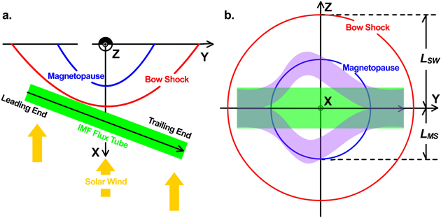
Figure 1. Geometries of the undisturbed and inclining IMF flux tube (green rectangles), the bow shock (red curves), and the magnetopause (blue curves) at the (a) Z = 0 and (b) X = 0 planes in the SWI coordinate system. The purple denotes the disturbed IMF flux tube split by the magnetopause, and the ±Y asymmetry is produced by the different magnetopause arrival times of the leading and trailing portions of the inclined IMF flux tube.
Download figure:
Standard image High-resolution imageTo determine the X-axis of the SWM and SWI, the solar wind velocities obtained from the OMNI data set are not directly used. Solar wind velocities are originally measured in the rest frame of the Sun–Earth system; the data in the OMNI data set, however, are given in the rest frame of the Sun–star inertial system, and the aberration velocity induced by the Earth's revolution around the Sun has been removed (∼29.8 km s−1 in the −Y direction in GSE). The solar wind velocities, which the magnetosphere feels, however, should be in the rest frame of the Sun–Earth system and include both the OMNI solar wind velocities and the revolution velocity. In this study, a 29.8 km s−1 velocity has been added back to the +Y component of the solar wind velocity in the GSE coordinate system.
2.3. Normalized Magnetosphere–Bow Shock System
The distribution of a parameter in the magnetosphere–bow shock space is hard to conduct, since the locations of the bow shock and magnetopause corresponding to each data point in the data set are different. To avoid this, each data point in this study has been relocated into a space with an averaged magnetopause and bow shock. In this normalized space, the radial direction of each data point (the latitude ϕ and longitude φ) and the ratio of the radial distances of each data point to the averaged magnetopause  and bow shock
  (
( ) remain the same as those in the original space.
The shape and location of the magnetopause and bow shock are described by the empirical models in this study. There are various magnetopause models, among which the axially symmetric model proposed by Shue et al. (1997) and the asymmetric model established by Lin et al. (2010) are the two popular ones. The latter can describe the asymmetric magnetopause with or without the polar cusp indentations, and the asymmetry is mainly induced by some intrinsic axial asymmetries, the polar indentations, and the dipole tilt. In our data set, 1573 magnetopause crossing events are identified by using the sharp changes in the plasma density, temperature, and velocity and the magnetic field. The distances to the X-axis, RYZ, of all of the events are plotted as a function of the X-coordinates in Figure 2(a), and the green, red, and blue curves are the cuts at the Y = 0 and Z = 0 planes in SWM of the averaged magnetopause modeled by Shue et al. (1997) and Lin et al. (2010), respectively. The distances of these events to the Earth are also plotted in Figures 2(b)–(d) as a function of the distances modeled by Shue et al. (1997; Figure 2(b)) and Lin et al. (2010) without (Figure 2(c)) and with (Figure 2(d)) the polar cusp indentations. The correlation analyses of these observed and modeled distances reveal that Lin et al.'s model with the polar cusp indentations can provide the best estimation of the magnetopause (Figure 2(d)). Lin et al.'s model with the polar indentations is thus adopted to calculate the radial distance of each data point to the magnetopause, DMP = rdata−rMP, where rdata is the distance of a data point to the Earth and rMP is the distance of the modeled magnetopause to the Earth along the radial direction of the data point.
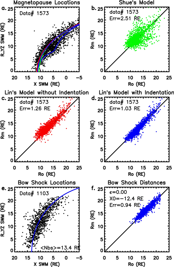
Figure 2. Locations of 1573 magnetopause crossing events and 1103 bow shock crossing events. (a) The distances to the X-axis, RYZ, of 1573 magnetopause crossing events are plotted as a function of the X-coordinates in SWM. The curves are the cuts at the Y = 0 and Z = 0 planes in SWM of the averaged magnetopause modeled by Shue et al. (1997; green) and Lin et al. (2010; red and blue), respectively. The radial distances of these events to the Earth, RO, are plotted as a function of the distances, RM, modeled by Shue et al. (1997; panel (b)) and Lin et al. (2010) without (panel (c)) and with (panel (d)) the polar cusp indentations. Lin et al.'s model with the polar cusp indentations provides the best estimation of the magnetopause, and the estimation error of 1.03 RE is smallest. (e) The distances of 1103 bow shock crossing events to the X-axis RYZ are plotted as a function of the X-coordinates, and the blue curve is the cut at the Y = 0 or Z = 0 plane in SWM of the averaged bow shock modeled by Fairfield (1971). (f) The radial distances of these bow shock crossing events to the Earth, RO, are plotted as a function of the modeled distances, RM.
Download figure:
Standard image High-resolution imageThe simple hyperbolic model proposed by Fairfield (1971) is used (see Equations (8) and (9)) to calculate the radial distance of a given data point to the bow shock, DBS = rdata−rBS, where rdata is the distance of a data point to the Earth and rBS is the distance of the modeled bow shock to the Earth along the radial direction of the data point. The standoff distance of the bow shock nose dn determines the size of the bow shock through L = (dn + x0)(1 + ε), and the focus location of the hyperbolic surface (x0, 0, 0) and the eccentricity ε determine the shape of the bow shock. The nose standoff distance dn is found to be a function of the upstream solar wind quantities, such as the magnetosonic Mach number, βSW, and the IMF orientation (Farris & Russell 1994), and the modeled nose standoff distances have been provided by the OMNI data set at a time resolution of 1 minute. The eccentricity ε and the focus location of the hyperbolic bow shock surface are generally considered to be constant and determined by seeking the best fit of the observed bow shock locations to the modeled locations. In our data set, we identified 1103 dayside bow shock crossing events by using the sharp changes in plasma density, temperature, and velocity and the magnetic field. The distances to the X-axis, RYZ, of all of the events are plotted as a function of the X-coordinates in Figure 2(e), and the blue curve is the cut at the Y = 0 or Z = 0 plane in SWM of the averaged bow shock modeled by Fairfield (1971). These bow shock crossing events are limited on the dayside, and the best fit of this data set to the hyperbolic model shown in Figure 2(f) gives ε = 0 and x0 = −12.4RE. The distance of a data point to the bow shock DBS is then calculated by adopting ε = 0 and x0 = −12.4RE, and the nose standoff distance dn is obtained directly from the OMNI data set.
After obtaining the location of a data point in the original space, including the latitude ϕ, longitude φ, and radial distances to the bow shock DBS and magnetopause DMP, the data point is then relocated into the normalized space described by an averaged bow shock and magnetopause. The input parameters to determine the averaged models are the averaged ones for all of the data in our database. When conducting statistics in the SWI coordinate system, for example, in Section 3.2, the averaged magnetopause is calculated through Lin et al.'s model without the polar cusp indentations. This is just for displaying the statistical data conveniently, since in SWI, the polar cusp indentations of the magnetopause are randomly rotated around the X-axis. When the statistics in the SWM coordinate system are performed, i.e., in Section 3.3, the averaged magnetopause is calculated through Lin et al.'s model with the polar cusp indentations. In the normalized space, the latitude ϕ, longitude φ, and distance ratio Rd of a data point remain the same as those in the original space, through which the normalized distances of the data point to the averaged bow shock and magnetosphere,  and
and  , can be obtained, and the data point is then relocated into the normalized space. Distributing parameters in this space are thus feasible, since all of the data points now have the identical averaged magnetopause and bow shock.
3. Statistical Results
3.1. External Conditions
The solar wind parameters, including the IMF orientation (θCL and θCO), plasma βSW, sound Mach number MS, and dipole tilt angle of the Earth θd, are determinative of the magnetosheath properties. In the data set of this study, the total number of data points is 2,318,978. The distributions of all solar wind and geomagnetic parameters corresponding to each data point are shown in Figure 3. The vector parameters in this figure are in the SWM or GSM coordinate systems.
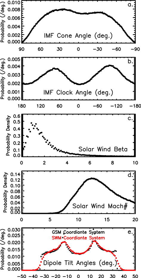
Figure 3. External conditions of the magnetosheath. Shown are the probability densities of (a) the IMF cone angle θCO, (b) the IMF clock angle θCL, (c) the solar wind plasma βSW, (d) the solar wind sound Mach number MS, and (e) the Earth's dipole tilt angle θd. All parameters are calculated in the SWM coordinate system except for the GSM dipole tilt angle θd, as shown in black in panel (e).
Download figure:
Standard image High-resolution imageThe IMF cone angle θCO controls the bow shock type on the magnetopause and thus is a key parameter determinative of the magnetosheath properties. Figure 3(a) shows the probability density of the IMF cone angle θCO calculated in SWM. According to its working definition in this study, θCO = ±90° indicates that the IMF is antiparallel and parallel to the direction of the incident solar wind, respectively, and θCO = 0° means the IMF is perpendicular to the solar wind velocity. It is seen that the IMF in the data set is mainly perpendicular or oblique to the Sun–Earth line ( < 60°) and that the radial IMF is relatively rare (
 > 60°). The mean of the absolute clock angle
  is 36°.
The IMF clock angle θCL controls the magnetic shear θX on the magnetopause and thus is critical to the occurrence of MR. The distribution of θCL is shown in Figure 3(b). It is not surprising to see that the probability density peaks roughly at ±90°, and this is the main feature of the Parker spiral IMF. It is worth noticing that, according to this distribution, the Y-axis of the instantaneous SWI coordinate system has a high probability of pointing in the dawn–dusk direction, and thus the Z-axis is nearly in the south–north direction in most cases.
The solar wind plasma βSW is another important parameter of the initiation and proceeding of MR on the magnetopause, and this parameter describes the relative contributions of the plasma and the magnetic field to plasma behaviors. The probability density of βSW is shown in Figure 3(c), and it is seen that βSW ranges mainly from 0 to 10 and peaks roughly at 1. This result suggests that in most cases, the plasma and the magnetic field in the solar wind are of equal significance.
The solar wind sound Mach number MS determines the bow shock strength and thus is critical to the magnetosheath properties. Figure 3(d) shows the probability density of MS in the data set. The MS is mainly greater than 5, and the distribution peaks at ∼12. In this large-MS situation, it is expected that the plasma compression and deceleration are almost the same for the different types of bow shocks as seen in Equations (6) and (7).
The dipole tilt angle θd, which sets the inner boundary conditions for the magnetosheath, is a key parameter to describe the symmetry of the magnetosphere. The black dots in Figure 3(e) show the occurrence probability of θd calculated in the GSM coordinate system (the angle between the Z-axis of GSM and the dipole axis), and it is seen that θd ranges between ±34° and peaks at roughly ±13°. When calculated in the SWM coordinate system, however, the range of θd expands from ±34° to more than ±50° (red dots in Figure 3(e)), although the occurrence probability of θd is very low at large angles. This is because the X-axis of the SWM is not fixed to the direction of the Sun but points against the instantaneous solar wind. That is to say, when the solar wind direction varies, the effective dipole tilt angle can be much larger than that expected in GSM, and the solar wind may hit the magnetosphere at a much higher magnetic latitude.
3.2. Statistics in SWI
The SWI coordinate system is related to the instantaneous solar wind velocity and the IMF but not the dipole axis of the Earth. The polar cusp indentations of the magnetopause are not located near the XZ plane but randomly distributed around the X-axis. For this reason, Lin et al.'s (2010) magnetopause model without the polar indentations is applied to calculate the averaged magnetopause and display the statistical data. The input parameters for the averaged model are the median quantities of the parameters in the data set, including the solar wind dynamic pressure Pdyn = 1.59 nPa, IMF BZ = 0.03 nT, IMF magnitude BT = 4.79 nT, and dipole tilt angle θd = 1°. For the averaged bow shock, the median value of the bow shock standoff distance dn = 13.6RE is input. The cuts of the modeled bow shock and magnetosphere at the planes with Y = 0 and Z = 0 are plotted by the red and white curves in Figure 4, respectively.
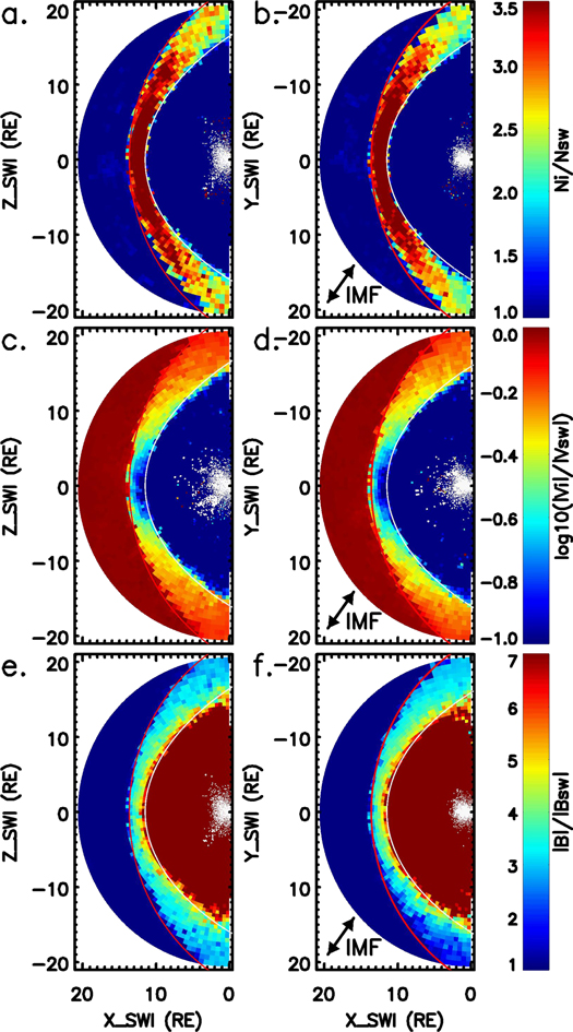
Figure 4. Cuts of the distributions of (a) and (b) the plasma density, (c) and (d) the velocity magnitude, and (e) and (f) the field magnitude at Y = 0 and Z = 0 in the SWI coordinate system. The arrows in panels (b), (d), and (f) denote the average IMF direction with the mean of the absolute cone angle  = 36°.
Download figure:
Standard image High-resolution imageFigure 4 shows the cuts of the distributions of the plasma density, velocity, and field magnitude at Y = 0 (the XZ plane; Figures 4(a), (c), and (e)) and Z = 0 (the XY plane; Figures 4(b), (d), and (f)). All of the data are normalized by the corresponding solar wind quantities ( ,
,  , and
, and  , where Ni,
  , and
, and  are the observed ion density, velocity, and magnetic field and NSW,
  , and
, and  are the corresponding solar wind density, velocity, and magnetic field). According to the definition of the SWI coordinate system, the IMF is always parallel to the Z = 0 plane and points to the directions of +X and +Y. The average of the absolute cone angle
  is 36°, which is denoted by the arrow in the XY planes in Figures 4(b), (d), and (f). It is seen that the magnetosheath, identified by the compression of both the plasma (Figures 4(a) and (b)) and the magnetic field (Figures 4(e) and (f)) and the plasma deceleration (Figures 4(c) and (d)), is embraced well by the averaged magnetopause (white curves) and bow shock (red curves). There are two main features in these distributions. First, both the deceleration and the compression are weaker at flanks or high latitudes than in the subsolar region, as seen in all of the distributions in Figure 4. This feature is produced by the parabolic shape of the bow shock, and the solar wind velocity component in the direction normal to the local magnetopause is smaller at flanks or high latitudes than in the subsolar region; i.e., the effective MS is smaller there, and thus the bow shock is weaker. The other feature is that there is a clear ±Y asymmetry present in the Z = 0 distribution of the field magnitude (Figure 4(f)), and the magnetic field behind the bow shock is compressed more significantly at the Y < 0 flank (by a factor of >3.5) than at the Y > 0 flank (by a factor of 1–2). When approaching the magnetopause at both the ±Y flanks, the field magnitude continues to increase. Notice that the IMF geometry related to the local bow shock at the ±Y flanks is different. Here ϕBS, which describes the IMF orientation relative to the normal of the local bow shock, is closer to 0° or 180° at the +Y flank and 90° at the −Y flank. The different types of bow shock, the quasi-parallel and quasi-perpendicular bow shocks, make this ±Y asymmetry. As is already known, the SWI Y-axes for most of the data points in the data set are near the dawn–dusk direction; thus, the ±Y asymmetries are in fact the dawn–dusk asymmetries produced by the Parker spiral IMF, as observed by Walsh et al. (2012) and Dimmock & Nykyri (2013). It should be noted that there is no clear ±Y asymmetry seen in the distributions of either plasma compression (Figures 4(a) and (b)) or plasma deceleration (Figures 4(c) and (d)), although the strong plasma compression region extends a little bit farther in the +Y direction than in the −Y direction, as seen in the dark red region in Figure 4(b).
In order to further explore the asymmetries of the magnetosheath plasma and magnetic field related to the IMF orientations, the distributions of sheath parameters in the YZ planes are particularly examined in Figures 5–12. Since the IMF geometry is the key factor to determine the bow shock types and makes the ±Y asymmetries, two subsets of the different IMF cone angles in the data set, i.e., the subsets with  < 30° and >60°, are particularly compared. The distributions of the plasma density are shown in Figure 5. Figures 5(a) and (b) show the distributions of the normalized ion density (
 ) in the YZ plane for the subset of
  < 30°. Figure 5(a) is the YZ projection of the distribution of the data located within a layer in the magnetosheath with a distance to the magnetopause greater than 1RE but less than 2RE. The blue and red curves are the intersections of the averaged magnetopause and bow shock with the X = 0 plane, denoting the terminator magnetopause and bow shock, respectively. The ±Y asymmetry can be seen in Figure 5(a), though it is very weak, and the plasma compression just in front of the terminator (the dayside magnetopause) is stronger at the +Y flank (marked in red) than that at the −Y flank (marked in yellow). This result is consistent with the data shown in Figure 4(b), where the strongest plasma compression region biases toward the +Y direction. Figure 5(c) is the same as Figure 5(a) but for the subset with
  > 60°. The ±Y asymmetry also appears in Figure 5(c), but this asymmetry is much weaker than the
  < 30° case, and it is able to be seen only behind the terminator (the nightside magnetopause): the green and yellow colors at the +Y flank denote a little stronger plasma compression than that at the −Y flank, marked in cyan and blue. The cuts of the distributions of
  at X = 0 are pretty uniform, as seen in Figures 5(b) and (d), indicating that this ±Y asymmetry is limited mainly in the region just outside of the magnetopause but not distant to it. The weak ±Y asymmetries in the plasma density distributions in Figures 5(a) and (c) cannot be produced by the different shock types, otherwise the plasma at the −Y flank could have been compressed more significantly than that at the +Y flank, according to Equations (6) and (7).

Figure 5. Distributions of the plasma density in the SWI coordinate system. (a) Projection on the YZ plane in SWI of the distributions of the normalized ion density ( , where Ni is the observed ion density and NSW is the corresponding solar wind ion density) for the subset of
  < 30°. All of the involved data points are located within a layer in the magnetosheath with a distance to the magnetopause greater than 1RE but less than RE. (b) Cut of the distributions of the normalized ion density at the X = 0 plane. The blue and red curves are the cuts of the averaged magnetopause and bow shock at X = 0, respectively. (c) and (d) Same as (a) and (b) but for the large cone angle subset of
  > 60°.
Download figure:
Standard image High-resolution imageThe asymmetries of the ion velocity are investigated in Figures 6 and 7 for the two subsets with  < 30° and
 >60°, respectively. The formats of these figures are the same as in Figure 5. The left column shows the YZ projections of the distributions of the magnitude and the components of the normalized ion velocity (
 ) within the layer in the magnetosheath with a distance to the magnetopause greater than 1RE but less than 2RE, and the right column shows the cuts of the velocity distributions at X = 0. From top to bottom in Figures 6 and 7, the parameters are
  ,
,  ,
,  , and
, and  . The first two parameters describe the plasma deceleration, and the last two parameters describe the plasma deflection. Here φdiv = 0° indicates that the sheath plasma is not diverted and still flows along the incident solar wind direction; φdiv = 90° means the sheath flow is diverted to the direction perpendicular to the incident solar wind. There are clear Y–Z asymmetries seen in the distributions of both the plasma deceleration and deflection, and the deceleration is stronger and the deflection weaker at the ±Y flanks than those at the ±Z flanks. These Y–Z asymmetries cannot be produced by the different types of shocks, since ϕBS at the ±Z flanks must be between the quantities of ϕBS at the +Y flank (ϕBS ∼ 0°) and −Y flank (ϕBS ∼ 90°), and the magnitudes of the deceleration and deflection at the ±Z flanks should also be between those at the ±Y flanks, which is clearly not what is seen in Figure 6. An additional mechanism must be present within the magnetosheath to reaccelerate the plasma at the ±Z flanks (Figures 6(b), (b'), (c), and (c')). The plasma deceleration does not show any clear ±Y asymmetry, but a weak ±Y asymmetry presents in the deflection; VYZ is smaller (Figures 6(c) and (c')), and, correspondingly, the deflection angle φdiv is smaller (Figures 6(d) and (d')) at the +Y flank than that at the −Y flank. The black arrows in Figures 6(c) and (c') show the direction of
  ; they basically point radially outward, and no clear asymmetry is presented.
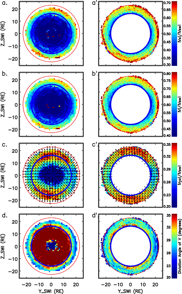
Figure 6. Distributions of the plasma velocity in SWI for the small cone angle subset of  < 30°. The formats are the same as in Figure 5. From top to bottom are
  ,
,  ,
,  , and the flow deflection angle
  , where
  is the observed ion velocity and
  is the corresponding solar wind velocity. The arrows indicate the plasma flow directions in the YZ plane.
Download figure:
Standard image High-resolution image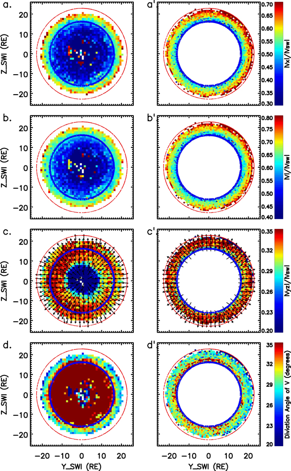
Figure 7. Distributions of the plasma velocity in SWI for the large cone angle subset of  > 60°. The formats are the same as in Figure 6.
Download figure:
Standard image High-resolution imageFor the large cone angle case in Figure 7, i.e.,  > 60°, the overall characteristic is that the deceleration is weaker than the small cone angle case if Figures 7(a), (a'), (b), and (b') are compared with Figures 6(a), (a'), (b), and (b'), respectively, while the flow deflection is stronger if Figures 7(c), (c'), (d), and (d') are compared with Figures 6(c), (c'), (d), and (d'), respectively. Both the Y–Z asymmetries and the ±Y asymmetries are not clear anymore in Figure 7, and only a weak ±Y asymmetry presents in Figure 7(c). The magnitude of the diverted flow at the +Y flank is weaker.
The comparison between Figures 6(b) and 7(b) indicates that the sheath flow is decelerated more significantly for the small IMF cone angle condition. As suggested by Cowley & Owen (1989), Cooling et al. (2001), and Swisdak et al. (2003), whether the sheath flow adjacent to the magnetopause is decelerated to be sub-Alfvénic is critical to the development of MR on the magnetopause. The "Alfvénicity" of the sheath flow within the layer with a distance to the magnetopause greater than 1RE but less than 2RE is examined in Figure 8 for the small IMF cone angle subset  < 30° and the large cone angle subset
  > 60°. Figure 8(a) shows the YZ projection of the distribution of the occurrence probability of the super-Alfvénic flow for the low IMF cone angle condition, and the blue in the subsolar region indicates that the flow in this region has a very low probability (<20%) of being super-Aflvénic. In this condition, MR may be easily initiated or proceed in a steady state. For the large cone angle condition (Figure 8(b)), the low probability region (blue) shrinks, and most of the observed flows on the magnetopause are super-Aflvénic.
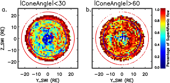
Figure 8. The YZ projection of the distribution of the occurrence probability of the super-Alfvénic flow for the subsets of  < 30° (a) and
  > 60° (b). All involved data points are located within the layer in the magnetosheath with a distance to the magnetopause greater than 1RE but less than 2RE.
Download figure:
Standard image High-resolution imageThe compression and bending of the magnetic field in the magnetosheath exhibit both the Y–Z and ±Y asymmetries for both of the two cone angle subsets. Figures 9 and 10 show the distributions of the magnetic field properties. The formats are also the same as in Figure 5. From top to bottom, the parameters are the normalized field magnitude  , the normalized YZ component of the magnetic field
  , the normalized X component of the magnetic field
  , and the field line bending angle in the XY plane
  . The arrows in the second row show the direction of the bent field in the YZ plane (φm,YZ). For the low cone angle case
  < 30°, the field compression exhibits clear Y–Z and ±Y asymmetries in Figures 9(a), (a'), (b), and (b'): the strongest field appears outside the dayside magnetopause in the Y < 0 region where, under the IMF geometry in SWI, the downstream of the quasi-perpendicular bow shock is, and the weaker field is found to be located in the Y > 0 region, downstream of the quasi-parallel bow shock. As seen in Figures 9(b) and (b'), in the region near the Y = 0 plane, either at the ±Z flanks or at the subsolar region, the arrows are basically along the +Y direction, which is the direction of the projection of the IMF on the YZ plane; the field lines are, however, divergent at the −Y flank and convergent at the +Y flank. These results show that when encountering the magnetosphere, an IMF flux tube in the solar wind (see the green region in Figures 1(a) and (b)) is locally split and bent by the magnetosphere (see the purple region in Figure 1(b)). The X component of the field
  and the angle φm,X in Figures 9(c), (c'), (d), and (d') describe the field line bending in the X direction. The magnitude of the X component is stronger at the ±Y flanks and almost zero near the Y = 0 plane. The distributions of the bending angles φm,X in Figures 9(d) and (d') exhibit a systematic pattern related to the IMF: at the −Y (+Y) flank the field line bends against (toward) the incident solar wind; in the region near Y = 0, the field lines are basically parallel to the YZ plane. Figure 9 is for the small IMF cone angle case, i.e.,
  < 30°, and even this small cone angle makes a difference in the bending angles between the ±Y flanks. The magnitude of BX is stronger, the area of the strong BX is wider at the −Y flank than at the +Y flank (Figures 9(c) and (c')), and the zero-bent field region (the green region in Figures 9(d) and (d')) is also biased from the Y = 0 plane toward the +Y flank.
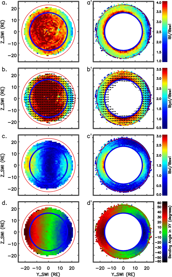
Figure 9. Distributions of the magnetic field in SWI for the small cone angle subset of  < 30°. The formats are the same as in Figure 5. From top to bottom are
  ,
,  ,
,  , and the field line bending angle in the XY plane
  , where
  is the observed magnetic field and
  is the corresponding IMF. The arrows in panels (b) and (b') show the direction of the bent field projected in the YZ plane (φm,YZ).
Download figure:
Standard image High-resolution image
Figure 10. Distributions of the magnetic field in SWI for the large cone angle subset of  > 60°. The formats are the same as in Figure 9.
Download figure:
Standard image High-resolution imageWhen the IMF cone angle is large (Figure 10), i.e.,  > 60°, the compression of the magnetic field is weaker, but the asymmetries in the field compression and field line bending are much more significant than those for the small cone angle case. The maximum
  is about 3.5 in Figures 10(a) and (a'), which is not so large as that for the
  < 30° case (over 4 in Figures 9(a) and (a')). The strong compression occurs at the −Y flank. The field line bending in the YZ plane is significantly asymmetric, and at the −Y flank, the projections of the fields are basically along the +Y direction, while at the +Y flank, they converge significantly toward the Z = 0 plane (Figures 10(b) and (b')). The field line bending in the XY plane also exhibits a significant ±Y asymmetry, as shown in Figures 10(d) and (d'), and the remarkable characteristics of the distribution of φm,X are that the zero-bent field line region (green region) is biased significantly to the +Y flank and that at the Y = 0 plane, the bending angles are +20° to +30°.
The plasma and magnetic pressures, Pi and Pm, are critical to the physics on the magnetopause, and they are investigated in Figures 11 and 12 for the small and large cone angle subsets, respectively. The same formats are used in these two figures as in Figure 5. All pressures are normalized by the corresponding solar wind dynamic pressure, Pdyn. From top to bottom in Figures 11 and 12 are the ion thermal pressure Pi/Pdyn, the magnetic pressure Pm/Pdyn, the proxy for the total pressure Pt = (2Pi + Pm)/Pdyn (the electron pressure is not good enough to conduct the statistics, and 2Pi is used to represent the total plasma pressure, which is the sum of the ion and electron pressures), and the ion β = Pi/Pm. Figure 11(a) shows that the ion pressure Pi is strong in the subsolar region. A weak asymmetry can be seen between the ±Y flanks, and the strong Pi region (green region) shifts toward the +Y flank a little bit. The strong magnetic pressure Pm is mainly located in front of the terminator outside the dayside magnetopause and a significant asymmetry presents: in the subsolar region and at the +Y flank, the magnetic pressure is weaker than that elsewhere on the dayside magnetopause (Figure 11(b)). The total pressure is strong on the dayside magnetopause and almost centrally symmetric (Figures 11(c) and (c')). The ion β distribution is asymmetric and larger in the subsolar region and at the +Y flank (Figures 11(d) and (d')), and this ±Y asymmetry is induced by the asymmetry of the magnetic pressure Pm (Figures 11(b) and (b')).

Figure 11. Distributions of the normalized pressures in SWI for the small cone angle subset of  < 30°. The formats are the same as those in Figure 5. From top to bottom are Pi/Pdyn, Pm/Pdyn, Pt = (2Pi + Pm)/Pdyn, and β = Pi/Pm, where Pi, Pm, and Pdyn are the ion thermal pressure, the magnetic pressure, and the corresponding solar wind dynamic pressure.
Download figure:
Standard image High-resolution image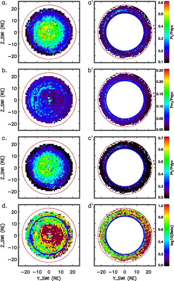
Figure 12. Distributions of the normalized pressures in SWI for the large cone angle subset of  > 60°.
Download figure:
Standard image High-resolution imageThe same ±Y asymmetries appear for the large cone angle case in the distributions of Pm and β in Figure 12. In the subsolar region and at the +Y flank, Pm is weaker and β is stronger than those elsewhere on the dayside magnetopause. Compared with the small cone angle case in Figure 11, the differences are remarkable: the area of the strong ion pressure Pi region in Figure 12(a) (green) expands in the subsolar region if compared with that of the  < 30° subset in Figure 11(a); the magnetic pressure is much weaker in Figure 12(b) (cyan and blue) than that in Figure 11(b) (green); the total pressure Pt is a little bit weaker in Figure 12(c), and the strong Pt region shrinks in Figure 12(c) compared with that in Figure 11(c), which is mainly due to the much weaker Pm in the region just before the terminator; the ion β is much larger over all of the magnetopause in Figures 12(d) and (d') (dark red) than that in Figures 11(d) and (d'); and the ±Y asymmetry is still present in Figures 12(d) and (d').
The variations of the plasma density, magnetic field magnitude, and plasma velocity along the X-axis in the subsolar magnetosheath (the distance to the X-axis is less than 6RE) are investigated in Figures 13, 14 and 15, respectively. The vertical black lines in these figures denote the positions of the averaged bow shock and magnetopause at X = 13.6RE and 11.1RE, respectively. In order to explore the dependences of the variations on the outside solar wind and IMF conditions, the data in these analyses are divided into different subsets by the IMF cone angles as shown in panel (a) (subsets with  ,
,  , and
, and  ), the IMF clock angles as shown in panel (b) (subsets with
  ,
,  , and
, and  ), the solar wind plasma βSW as shown in panel (c) (subsets with βSW < 1, 1 < βSW <2, and βSW > 2), and the solar wind convection electric field
  shown in panel (d) (subsets with
  ,
,  , and
, and  mV m−1). The solar wind sound Mach number MS is not used to classify the data set because MS values in the data set are basically greater than 5, as shown in Figure 3(d), and in this situation, the deceleration and compression of plasma through the bow shock in the subsolar region are almost independent of MS according to Equations (6) and (7). This paper tries to touch on the questions of how fast and where magnetic flux is reconnected on the magnetopause. The solar wind convection electric field
  is involved, since it describes how fast the IMF flux is transported toward the bow shock and the magnetospheric system. When the IMF cone angle θCO is large, that is,
  is almost along or against the direction of
  , the uncertainty of the calculation of the solar wind convection electric field
  increases. For this reason, only the data with
  are involved in Figures 13(d), 14(d), and 15(d). The colored curves in these figures show the spline regression of the studied parameters on the X-coordinate for all subsets, and these regressions are performed by using the public R statistical software (R Core Team 2019).
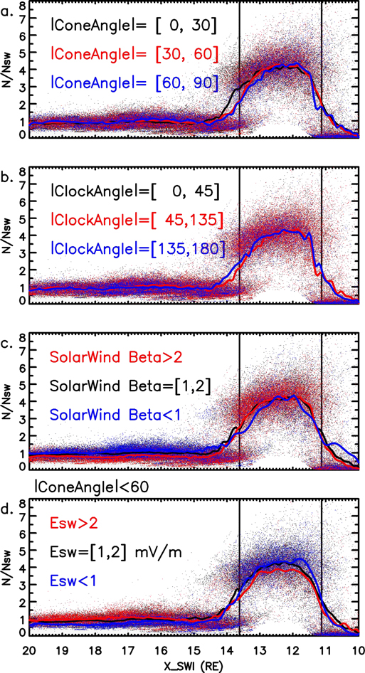
Figure 13. Profiles of the normalized ion density  along the X-axis in SWI for the subsets of different (a) IMF cone angle θCO, (b) IMF clock angle θCL, (c) solar wind plasma βSW, and (d) solar wind convection electric field ESW. All involved data points are confined in the subsolar region with the distances to the X-axis less than 6RE. The curves show the regression of
  on the X-coordinate for the different subsets.
Download figure:
Standard image High-resolution image
Figure 14. Profiles of the normalized field magnitude  along the X-axis in SWI for the subsets of different (a) IMF cone angle θCO, (b) IMF clock angle θCL, (c) solar wind plasma βSW, and (d) solar wind convection electric field ESW. All involved data points are confined in the subsolar region with distances to the X-axis less than 6RE. The curves show the regression of
  on the X-coordinate for the different subsets.
Download figure:
Standard image High-resolution image
Figure 15. Profiles of the X component of the plasma velocity  along the X-axis in SWI for the subsets of different (a) IMF cone angle θCO, (b) IMF clock angle θCL, (c) solar wind plasma βSW, and (d) solar wind convection electric field ESW. All involved data points are confined in the subsolar region with distances to the X-axis less than 6RE. The curves show the regression of
  on the X-coordinate for the different subsets.
Download figure:
Standard image High-resolution imageThe overall profiles of the normalized ion density  along the X-axis are almost identical for all but the subsets with different
  in Figure 13. The ion density increases at the bow shock at X = 13.6RE, which is due to the strong compression of the bow shock. Here
  continues to increase behind the bow shock and peaks roughly at X = 12RE, and this increase results from the pileup of the shocked plasma against the magnetopause. Behind X = 12RE but before the averaged magnetopause, the ion density drops suddenly, and this sudden decrease possibly stands for the depletion layer just ahead of the magnetopause, or it may just derive from the error of determining the location of the bow shock, since the error of the modeled bow shock location is about 1RE (Figure 2(f)), that is to say, some of the data behind X = 12RE and in front of the average magnetopause are actually located in the magnetosphere in the original space. These two possibilities cannot be distinguished in the present analysis. None of the outside conditions but the solar wind convection electric field
  make a clear difference among their corresponding subsets. It is clear in Figure 13(d) that the plasma pileup effect is less significant for the large
  subset, and the profile of
  for the large
  becomes flat at the location very close to the bow shock (at X = 13RE), as shown by the red curve in Figure 13(d). The pileup effect is most significant for the smallest
  subset, and the density profile keeps increasing until deep into the magnetosheath and peaks roughly behind X = 12RE. The profile with the median quantity of
  (black curve) is located between the profiles with the large and small
  in Figure 13(d).
The field magnitude jumps at the bow shock at X = 13.6RE, continues to increase gradually when heading toward the magnetopause, and jumps abruptly again at roughly X = 12RE for all subsets shown in Figure 14. As mentioned previously, the second abrupt increase in the field magnitude ∼1RE ahead of the magnetopause may be attributed to the depletion layer or the error of estimating the location of the magnetopause. The IMF cone angle θCO makes the remarkable difference among the profiles of the field magnitude of the subsets shown in Figure 14(a): for the small cone angle case of  , the quasi-perpendicular bow shock in the subsolar region compresses the magnetic field most efficiently by a factor of ∼4, and the whole profile of the field magnitude (black curve) is above those of all other subsets; for the large cone angle case of
  , the quasi-parallel shock in the subsolar region almost does not compress the magnetic field, and the whole profile is lowest (blue curve); for the middle cone angle case of
  , the field magnitude profile is in the middle (red curve). The solar wind plasma βSW (Figure 14(c)) and convection electric field
  (Figure 14(d)) also make differences among their subsets. When heading toward the magnetopause, the magnetic field pileup effect is least significant for the smallest βSW or strongest
  : the field magnitude increases slower than the other subsets, as shown by the blue curve in Figure 14(c) and the red curve in Figure 14(d). These differences among the subsets do not begin right at the bow shock but appear in the magnetosheath on the way to the magnetopause, suggesting that the magnetosheath internal process or the process on the inner boundary, i.e., the magnetopause, may produce these differences.
The difference among the subsets made by the solar wind βSW and the convection electric field  are also seen in the velocity profiles
  in Figure 15. Although the velocity profiles for all subsets in Figure 15 decrease all the way from the bow shock to the magnetopause, the velocity is faster at any location in the magnetosheath for the smaller βSW or stronger
  subsets: the velocity profiles for the smaller βSW (βSW < 1, as shown by the blue curve in Figure 15(c)) and the stronger
  (
( mV m−1, as shown by the red curve in Figure 15(d)) are above those of the other subsets.
It is traditionally thought that MR tends to occur or proceed faster when the IMF clock angle θCO is large, and it is thus expected to see that the pileup effect may also be less significant under a larger IMF clock angle condition (Phan et al. 1994). The data shown in Figures 13(b), 14(b), and 15(b) demonstrate, however, that there is no systematic difference among the profiles of the subsets of different IMF clock angles.
3.3. Estimation of IMF Magnetic Flux Going through the Magnetosphere
By taking advantage of the SWI coordinate system, a method is proposed to roughly estimate how much IMF magnetic flux goes through the magnetosphere via MR on the magnetopause. When a flux tube embedded in the solar wind encounters the magnetopause, the IMF field lines within the flux tube have two ways to return back to the solar wind. One way is that the IMF field lines reconnect with the magnetospheric field lines through MR on either the low- or high-latitude magnetopause, and this way can be termed "going through the magnetosphere"; the other way is that the IMF field lines are bent in front of the magnetopause and diverted into the flank magnetosheath, and in this way, the IMF field lines directly come back to the downstream solar wind. By calculating the total magnetic flux in the solar wind rushing toward the bow shock per unit time (FSW) and the magnetic flux diverted into the flank magnetosheath per unit time (FSH), the magnetic flux going through the magnetosphere via MR on the magnetopause can be estimated by FR = FSW − FSH. The SWI coordinate system is convenient for performing this estimation. In the SWI coordinate system, the flux tube in the solar wind is aligned in the X and Y directions. Let us assume that the width of the flux tube in the solar wind is equal to the dimension of the terminator bow shock in the Z direction, LSW (as shown in Figure 1(b)). This width can be estimated by the bow shock model for each data point in our data set. Assuming that the solar wind velocity and the IMF are uniform within the scale of LSW, the total flux in the solar wind FSW can be estimated directly via FSW = VSW,XBSW,YLSW. The width of the magnetosheath at the ±Z flanks in the terminator plane can be estimated via LSH = LSW − LMS, where LMS is the width of the terminator magnetopause in the ±Z directions. If the convection electric field in the sheath EX = VXBY is uniformly distributed along the ±Z directions at the terminator, the total flux flowing from the flank magnetosheath into the downstream solar wind per unit time can be estimated via FSH = EXLSH. After that, the total magnetic flux going through the magnetosphere per unit time via MR can be calculated by FR = FSW − FSH. It should be noted, however, that the dimension parameters involved in this calculation, i.e., the widths of the magnetopause and the bow shock along the Z-axis at the terminator plane, are modeled, and thus the errors may enter into the calculation.
To perform the aforementioned estimation of FR, the key constraint is that the convection electric field in the sheath, EX = VXBY, should be constant along the ±Z directions, and only in this condition can the total flux be estimated simply via FSH = EXLSH, instead of integrating EX along the Z direction in the sheath. Figure 16 shows the cuts of the distributions of the electric field at the terminator plane X = 0. The data set is divided by the IMF cone angle θCO into two subsets with  and
and  , and the two subsets are shown in the left and right columns, respectively. From top to bottom of each column are the electric field magnitude normalized by the solar wind convection electric field,
  ; the electric field component describing the flux transport in the X direction,
  ; and the electric field component describing the flux transport outward in the YZ plane,
  . Data in Figure 16 indicate that the transport of the magnetic flux is mainly in the X direction for both the large and the small cone angle subsets. Here
  and
and  exhibit clear Y–Z asymmetries, and they are stronger at the ±Z flanks than those at the ±Y flanks. Also presenting weak ±Y asymmetries are
  and
and  , and they are a little bit stronger at the −Y flank. These asymmetries mainly derive from the asymmetries of the distributions of the magnetic field as shown in Figures 9(b') and 10(b'). The one important characteristic is that
  is pretty constant along the ±Z directions at the ±Z flanks near Y = 0, at least for the low cone angle case as shown in Figure 16(b). For the large cone angle case shown in Figure 16(b'), however, the small angle between the incident solar wind and the IMF introduces an uncertainty in the calculation of
  , and
, and  is not that constant along the ±Z directions at the ±Z flanks near Y = 0. The uniform
  along the Z-axis allows us to calculate FSH, and thus FR.
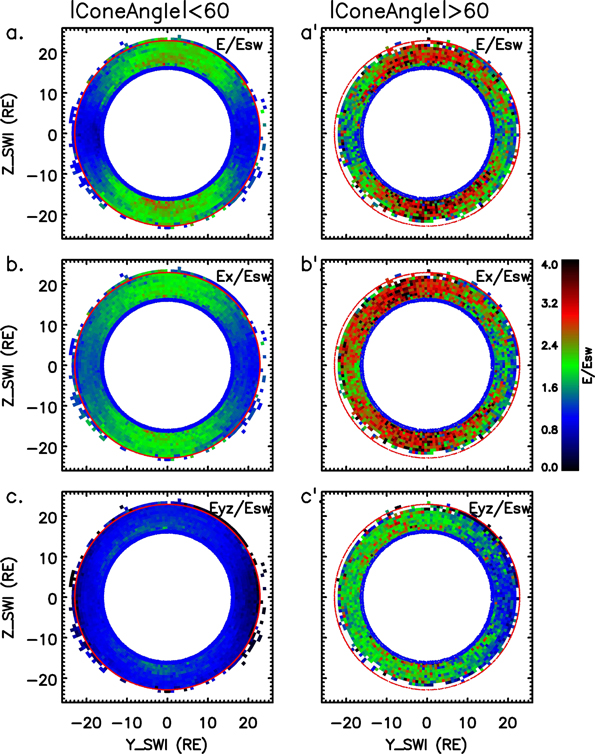
Figure 16. Cuts of the distributions of the electric field parameters at the terminator plane X = 0 in the SWI coordinate system. The left and right columns are for the subsets of  < 60° and >60°, respectively. From top to bottom are (a)
  , (b)
, (b)  , and (c)
![${E}_{{YZ}}/\left|{{\boldsymbol{E}}}_{\mathrm{SW}}\right|=| [0,{V}_{Y},{V}_{Z}]\times {\boldsymbol{B}}| /| {{\boldsymbol{E}}}_{\mathrm{SW}}| $](https://content.cld.iop.org/journals/0004-637X/880/2/122/revision1/apjab290eieqn162.gif) .
.
Download figure:
Standard image High-resolution imageFigure 17 shows the distributions of the calculated FR, the magnetic flux going through the magnetosphere per unit time, as functions of the outside solar wind and IMF conditions. The data used to calculate FR are observed in the magnetosheath at the ±Z flanks with  < 3RE and
  < 5RE, and the distances to the magnetopause and bow shock are greater than 0.5RE. In each plot of Figure 17, the red curves are the splines regression of FR on the IMF cone angle θCO (Figure 17(a)), the absolute IMF clock angle
  (Figure 17(b)), the IMF strength
  (Figure 17(c)), the solar wind plasma βSW (Figure 17(d)), the solar wind electric field
  (Figure 17(e)), and the solar wind sound Mach number MS (Figure 17(f)). The regressions here are also performed by using the public R software (R Core Team 2019). Despite the significant scattering of the data, it is clearly seen that more magnetic flux goes through the magnetosphere when
  is smaller,
  is stronger, βSW is smaller,
  is stronger, or MS is smaller, as shown in Figures 17(a), (c), (d), (e), and (f). The control of the IMF clock angle, θCL, to FR is seen in Figure 17(b): when
  > 90°, the larger the
  , the more magnetic flux FR is reconnected (at the top of Figure 17(b)). When
  < 90°, however, FR tends to decease when
  increases toward 90° (at the bottom of Figure 17(b)). In fact, the high-latitude lobe reconnection may occur at high latitudes behind the polar cusps when θCL is small and the IMF flux may go through the magnetosphere via the dual high-latitude lobe MR (Song & Russell 1992).
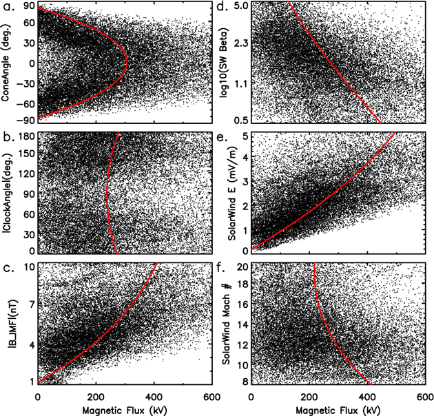
Figure 17. Estimated magnetic flux going through the magnetosphere per unit time FR vs. the IMF cone angle  (a), IMF clock angle
  (b), IMF magnitude
  (c), solar wind βSW (d), solar wind convection electric field ESW, (e) and solar wind sound Mach number MS. All data points involved in the calculation are observed in the magnetosheath at the ±Z flanks with
  < 3RE and
  < 5RE, and their distances to the magnetopause and bow shock are greater than 0.5RE. The red curves are the regressions of FR on the different conditions.
Download figure:
Standard image High-resolution imageThere are less data points distributed near θCL = 90° in Figure 17(b). The observing satellites, either Cluster or THEMIS, are typically located in the dawn or dusk flanks in the GSM (or SWM) coordinate system when they fly through the terminator. In this condition, when  ∼ 90°, these satellites have little chance to be located at the ±Z flanks in the SWI coordinate system, since this region is actually the high-latitude terminator region in GSM (or SWM) where the observing satellite cannot enter.
3.4. Statistics in SWM
The SWM coordinate system, similar to the GSM coordinate system, is related to the magnetic dipole axis of the Earth. The dipole axis always lies in the Y = 0 plane, it may be parallel or oblique to the Z-axis of SWM, and the angle between them is the dipole tilt angle θd. The magnetosheath asymmetries present in SWI should be smoothed out in the SWM coordinate system, since the IMF orientations are now randomly distributed. The geometry of the magnetic dipole thus can be a source to induce the magnetosheath asymmetries in SWM.
Figure 18 shows the YZ projections of the distributions of the pressures within a layer outside the magnetopause with distances to the magnetopause greater than 1RE and less than 2RE (left column) and another layer inside the magnetopause with distances to the magnetopause less than 1RE (right column). All pressure quantities in Figure 18 are normalized by the corresponding solar wind dynamic pressures, Pdyn. The ion pressure outside the magnetopause, Pi/Pdyn, is shown in Figure 18(a). A strong Pi/Pdyn region is located at low latitudes (cyan and green), and this region extends wider along the dawn–dusk direction than the south–north direction. The maximum Pi/Pdyn occurs in the subsolar region, and its quantity reaches 0.45. Theoretically, the plasma thermal pressure Pth, i.e., the sum of the ion and electron pressures (Pi + Pe), should be ∼89% of the incident solar wind pressure (Pth/Pdym = ∼0.89; Margaret G. Kivelson 1995). The maximum quantity of 0.45 is about half the theoretical value, which is reasonable since only the ion pressure is involved. The magnetic pressure Pm/Pdyn just outside the magnetopause is below 0.2 (Figure 18(b)), and it is much weaker than the ion pressure. The strongest magnetic pressure is not present in the subsolar region but at the higher latitudes. This result is consistent with what is seen in SWI in Figures 11(b) and 12(b), and there the statistics show that the strongest magnetic pressure occurs at the −Y flank and the bias may be attributed to the nonzero IMF cone angle. The total pressure is hard to obtain in this study, since the electron pressure is not good enough, and Pt = (2Pi + Pm)/Pdyn is plotted in Figure 18(c) as a proxy for the total pressure. It is seen that the distribution pattern of Pt is similar to that of Pi in Figure 18(a). The ion β outside the magnetopause is plotted in Figure 18(d), and it shows that the maximum β is as large as 10 and the high β is limited within a belt at the low latitudes.
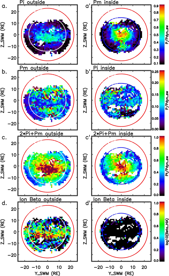
Figure 18. The YZ projections of the distributions of the pressures within a layer outside the magnetopause with distances to the magnetopause greater than 1RE and less than 2RE (left column) and a layer inside the magnetopause with distances to the magnetopause less than 1RE (right column). Here Pi/Pdyn, Pm/Pdyn, Pt = (2Pi + Pm)/Pdyn, and β = Pi/Pm are displayed in the SWM coordinate system, where Pi, Pm, and Pdyn are the ion thermal pressure, magnetic pressure, and corresponding solar wind dynamic pressure.
Download figure:
Standard image High-resolution imageFigures 18(a') and (b') show the magnetic and ion pressures inside the magnetopause, respectively. The strong magnetic pressure region is located at low latitudes and extends more in the dawn–dusk direction than in the south–north direction (Figure 18(a')), the pattern of which is similar to those of the ion and the total pressures outside the magnetopause. The maximum magnetic pressure occurs in the subsolar region, and the quantity reaches ∼0.9. The ion pressure inside the magnetopause is mostly below 0.15, as shown in Figure 18(b'), leading to the very low ion β just inside the magnetopause, as shown in Figure 18(d'). The total pressure inside the magnetopause is dominated by the magnetic pressure, and its magnitude is comparable with that of the total pressure outside the magnetopause, as shown in Figures 18(c) and (c').
The flow pattern in the magnetosheath is investigated in Figure 19. All of the data involved are in the layer outside the magnetopause. Figure 19(a) displays the distribution of the occurrence probability of the positive VZ (hereafter referred to as the "VZ polarity"). A VZ polarity equal to 1 means that the flows at this location are all northward, and a zero VZ polarity means that the flows there are all southward. Data in Figure 19(a) indicate that the VZ polarity is almost 1 in the northern hemisphere (red) and zero in the southern hemisphere (blue). The transition region marked by cyan and green (the VZ polarity is ∼0.5) between the red and blue regions is located at the equator and very narrow. This narrow transition region suggests that the location of the line separating the northward and southward plasma flows is fixed near the equator and is not controlled by the dipole tilt angles, otherwise the randomly distributed dipole tilt angle θd may make a wider transition region between the red and blue regions.

Figure 19. Magnetosheath flow characteristics in the SWM coordinate system. (a) The YZ projections of the distribution of the occurrence probability of the positive VZ in the SWM coordinate system. (b) The YZ projections of the distribution of the occurrence probability of the super-Alfvénic flow. All of the involved data are located within a layer outside the magnetopause, with the distances to the magnetopause greater than 1RE and less than 2RE.
Download figure:
Standard image High-resolution imageThe "Alfvénicity" of the sheath flow is examined in the SWM coordinate system, and the probability of the super-Alfvénic flow outside the magnetopause is shown in Figure 19(b). The data are the same as those in Figure 8. The lowest occurrence probability of the super-Alfvénic flow (<20%) appears around the subsolar region; at high latitudes near the noon meridian plane, the occurrence probability increases to above 50%; and at the dawn and dusk flanks ( > ±7RE), the sheath is almost always super-Alfvénic, and the occurrence probability is almost 100%.
The dependences on the dipole tilt angle of the patterns of the ion and magnetic pressure distributions are examined in Figure 20. The data involved in this figure are located within the two layers just outside or inside the magnetopause, and they are the same as in Figure 18 but are confined around the noon meridian with  < 10RE. Here Pi/Pdyn, β, and the VZ polarity outside the magnetopause and Pm/Pdyn both inside and outside the magnetopause are plotted as functions of the latitudes in SWM and the dipole tilt angle θd in Figure 20. A data gap is present in the southern hemisphere (negative latitudes) for all plasma data outside the magnetopause, and this is due to lack of plasma data on Cluster-4. A ridge clearly appears in Figure 20(a) for Pi/Pdyn outside the magnetopause (dark red), and when the dipole axis rotates toward the Sun (θd increases from −34° to 34°), the maximum pressure region on the magnetopause shifts southward from the northern hemisphere to the southern hemisphere (the latitudes of the maximum pressure region decrease). In the magnetic pressure plot in Figure 20(b), a valley is present near the magnetic equator (blue), and when the dipole axis rotates toward the Sun, the magnetic pressure valley outside the magnetopause also shifts southward along with the ion pressure ridge. Both the ion β outside the magnetopause and the magnetic pressure inside the magnetopause exhibit a ridge near the magnetic equator, and the same controls of the dipole tilt angle θd to these two quantities are seen clearly in Figures 20(c) and (d). The VZ polarity outside the magnetopause shown in Figure 20(e) confirms the observations in Figure 19(a), and the line separating the northward and southward flows is always located at the equator plane of SWM, no matter what the dipole tilt angle is.

Figure 20. Distributions of Pi/Pdyn, Pm/Pdyn, β = Pi/Pm, and the occurrence probability of the positive VZ as a function of the latitudes in SWM and the dipole tilt angles. All of the data outside the magnetopause are located within a layer in the magnetosheath with distances to the magnetopause greater than 1RE and less than 2RE and confined in the region around the noon meridian with  < 10RE. All of the data inside the magnetopause are located within a layer in the magnetosphere with distances to the magnetopause less than 1RE and confined within
  < 10RE.
Download figure:
Standard image High-resolution image4. Discussion
The magnetosheath parameters, particularly those quantities adjacent to the magnetopause, control the initiation and progress of MR and determine where and how fast MR proceeds on the magnetopause. The key magnetosheath parameters include the magnetopause current density jMP (Pudovkin & Semenov 1985; Alexeev et al. 1998); the magnetic shear θX (Trattner et al. 2007); the magnetosheath field  and plasma density ρ (Cassak & Shay 2007; Liu et al. 2018); the magnetosheath plasma β, which describes the combination effect of
  and ρ (Sonnerup 1974; Swisdak et al. 2003; Phan et al. 2013); the Alfvén velocity VA (Cowley & Owen 1989; Cooling et al. 2001; Swisdak et al. 2003); and the sheath flow velocity
  (Raeder 2006). The magnetopause current jMP and the magnetic shear θX cannot be determined by in situ observations of a single satellite. In this study, jMP is investigated by using a proxy, the thermal pressure Pth outside the magnetopause, and a stronger thermal pressure in the magnetosheath may indicate a stronger magnetopause current jMP, which balances with the stronger thermal pressure outside. Here θX is explored by using the asymmetric distribution of the bending of the magnetosheath magnetic field lines
  . In addition, all of these parameters are not necessarily independent; for example, VA may relate to β (Swisdak et al. 2003), and both of them represent the combination effect of
  and ρ. It is hard to investigate these parameters right at the location where MR occurs; thus, the statistics in this study can provide a magnetosheath background for the initiation or proceeding of MR. Although MR can reduce the size of the obstacle, i.e., relocate the magnetopause, and thus modifies the magnetosheath properties (Aubry et al. 1970; Phan et al. 1996), fortunately, in a quasi-steady state, MR itself does not change the upstream magnetosheath properties significantly (Borovsky et al. 2008). That makes the statistics of the background magnetosheath meaningful.
In this study, by distributing the observations in a rescaled space with an average bow shock and magnetopause, the abovementioned magnetosheath properties related to the magnetopause MR are investigated. Two different coordinate systems, SWI and SWM, are adopted to reveal the asymmetries produced by the IMF, which is the outer boundary condition for the magnetosheath, and the asymmetries produced by the Earth's dipole tilt, which acts through modifying the inner boundary of the magnetosheath. The X-axes of both coordinate systems point against the instantaneous solar wind direction, and in this way, the biases induced by the solar wind direction have been removed.
The statistical magnetosheath properties in this study can be classified into three groups relating to three aspects of MR on the magnetopause. To what extent can the solar wind and IMF conditions stand for the inflow condition of MR on the magnetopause? What parameters in the upstream solar wind affect the MR rate on the magnetopause? And what parameters affect the locations of MR on the magnetopause?
4.1. Magnetosheath Asymmetries Related to the IMF Orientation
The magnetosheath properties of both the plasma and the magnetic field are investigated in the SWI coordinate system. These parameters include  , ρ, Pi, β, VA, and
  . There are two kinds of asymmetries existing in the distributions of these studied parameters, the ±Y asymmetries and the Y–Z asymmetries, and they are produced by different mechanisms.
The ±Y asymmetries are mainly present in the magnetic field quantities. The field magnitude  exhibits a clear ±Y asymmetry in Figure 4(f). This asymmetry is produced by the different types of bow shock at the opposite flanks. Due to the parabolic shape of the bow shock and the geometry of the IMF in the SWI coordinate system (
 = 36°), ϕBS, which describes the IMF orientation relative to the normal direction of the local bow shock, is different at the ±Y flanks. At the +Y flank in SWI, ϕBS is closer to 0° or 180°; thus, the bow shock there is the quasi-parallel shock, which cannot compress the magnetic field significantly (see Equation (6)). At the −Y flank, ϕBS is closed to 90°, and the quasi-perpendicular bow can compress the magnetic field by a factor up to 4 (see Equation (7)). This asymmetry in the magnetic field compression creates the asymmetries in all of the magnetic field–related parameters, such as the field components
  and
and  , field bending angle φm,X, magnetic pressure Pm, and plasma β. Clearly, these asymmetries are all controlled by the IMF cone angle θCO if comparing Figures 9 and 11 with Figures 10 and 12, respectively.
The ±Y asymmetries for the plasma parameters, however, are very weak, and this is understandable because the solar wind Mach number MS is large. Figure 3(d) shows that most of the MS values in the current data set are greater than 5, and the occurrence probability density peaks at MS ∼ 12. According to Equations (6) and (7), the compression and deceleration of plasma do not depend on either the type of the bow shock (ϕBS) or the Mach number (MS) strongly if MS is big enough. That is why the different types of bow shock have not decelerated and compressed the plasma differently at the ±Y flanks. In fact, according to the shock theory, the quasi-parallel bow shock at the +Y flank should make less decelerated (faster) and more tenuous plasma. This faster plasma has been seen at the +Y flank just inside the terminator shock (the red region inside the terminator shock at the +Y flank in Figures 7(a') and (b')). In this terminator region, the component of the incident solar wind velocity in the direction normal to the local magnetopause is much smaller than that in the subsolar region; thus, the effective Mach number (MS) is small, and in this condition, the quantity of MS acts in Equation (6). Except for this terminator region, the slightly denser and slower plasma is seen in the magnetosheath at the +Y flank (Figures 4(b), 5(a) and (c), 6(c) and (c'), 7(c)). The magnitude of the flow diversion is also less significant at the +Y flank than at the −Y flank (Figures 6(d) and (d')). These weak ±Y asymmetries can be attributed to the continuous deceleration, compression, and diversion processes within the magnetosheath when the shocked solar wind and IMF continue to head toward the magnetopause. The more bent magnetic field lines within the +Y flank sheath may play a role in further blocking the plasma there (Figures 9(d) and 10(d)). The strongly compressed magnetic field within the −Y flank sheath may squeeze the plasma out and reduce the plasma density there. In this case, i.e., the IMF cone angle θCO is not zero, the most significant depletion effect (Phan et al. 1994) may not be located in the subsolar region but biases toward the −Y flank in the SWI coordinate system (Figure 5(a)).
The magnetosheath internal processes can also create the ±Y asymmetries of the magnetic properties. Here φm,YZ, which describes the bending of the magnetosheath field line in the YZ plane and is determinative of the magnetic shear θX on the magnetopause, exhibits a clear ±Y asymmetry that is observed to be controlled by the IMF θCO but not related to the different types of bow shocks. For the zero  case, it is expected to see that the field line bending in the Y–Z plane is symmetric at the ±Y flanks of the magnetopause. When an IMF flux tube with
  moves toward the magnetopause, it is initially split at the subsolar region, and the field lines diverge at the −Y flank and converge at the +Y flank. For the small
  case, the initial split point shifts a little bit toward the −Y flank, and it can be seen that at the +Y flank, the convergence of the sheath magnetic field lines is more significant than the divergence at the −Y flank (arrows in Figures 9(b) and (b')). For the large
  case in Figures 10(b) and (b'), this difference in the field line bending between the ±Y flanks is much more remarkable. When an IMF flux tube inclining toward the Sun (nonzero cone angle
  ) encounters the bow shock (green rectangles in Figure 1), the leading end of the flux tube touches the magnetopause first at the −Y flank, and this portion of the flux tube is split into two flux tubes (purple region in Figure 1(b)). In this region, the field lines basically lie on the magnetopause and are bent a little in the Y–Z plane. That is why the field line bending in the YZ plane is always slight at the −Y flank regardless of whether the cone angle θCO is large or small. As the flux tube continues to move, more and more portions of the flux tube touch the magnetopause. The newly split point of the flux tube moves further toward the +Y flank and the trailing end of the flux tube, where the magnetic field lines of the flux tube are close to the normal direction of the local magnetopause, and thus are bent significantly by the magnetopause. That is why the field line convergence at the +Y flank is more remarkable than the divergence at the −Y flank, particularly when the IMF cone angle
  is large.
The magnetosheath internal processes also make the Y–Z asymmetries of the magnetosheath. All components of the plasma velocity, i.e.,  ,
,  , and
, and  , exhibit clear Y–Z asymmetries (e.g., Figure 6), and the plasma is faster at the ±Z flanks than at the ±Y flanks, indicating an additional accelerating mechanism present in the magnetosheath at the ±Z flanks, and the tension force exerted by the bent sheath magnetic field may have acted to reaccelerate the plasma there (Figures 9 and 10). The shocked plasma is continuously diverted in the magnetosheath, and it convects the magnetic flux toward the ±Z flanks; that is why the field magnitude is much stronger at the ±Z flanks than at the ±Y flanks (Figure 9). The faster plasma and stronger magnetic fields leads to the stronger electric field within the magnetosheath at the ±Z flanks (Figure 16).
It should be mentioned that the asymmetries presented here are discussed in the SWI coordinate system and related to the IMF flux tube directions. In this coordinate system, the level of the asymmetries is controlled only by the IMF cone angle θCO. If discussed in the SWM coordinate system, these asymmetries should still be related to the direction of the IMF flux tube, but they are determined by both the IMF clock angle θCL and the cone angle θCO.
Thus, one must be very cautious to use the single solar wind and IMF conditions as a substitute for the conditions in the magnetosheath adjacent to the magnetopause, particularly when trying to pursue the answers to questions like where MR occurs on the magnetopause or how fast MR goes. For example, the magnetic field bending can be very different over the magnetopause, and thus the magnetic shear θX varies significantly, particularly for an IMF with a large  a strong asymmetry is also present in the distribution of the plasma β. Notice that both θX and β are critical to the initiation or proceeding of MR on the magnetopause (Sonnerup 1974; Swisdak et al. 2003; Trattner et al. 2007; Phan et al. 2013). The strong plasma β outside the subsolar magnetopause may suggest that it is not likely to contain fast MR.
4.2. Magnetopause Expansion under a Radial IMF Condition
A by-product that is the variation of the magnetopause flaring angle under the different IMF cone angle θCO is obtained by comparing the distributions for the small and large  . When the IMF cone angle increases from
  < 30° to >60°, it is seen that the total pressure Pt decreases and the strong Pt region shrinks in the subsolar region (Figures 11(c) and 12(c)). These variations of Pt are mainly because of the decrease in Pm (Figures 11(b) and 12(b)), and, in fact, the ion thermal pressure Pi remains unchanged, and the strong plasma compression region (Ni and Pi) even expands (compare Figures 5(a) and 11(a) with Figures 5(c) and 12(a), respectively). The Pm decreases because the quasi-parallel bow shock dominates over a wider region around the subsolar region when the IMF changes to be radial (
 > 60°) and, as is well known, the quasi-parallel bow shock does not compress the magnetic field significantly. The decrease in Pm thus results in a larger β (Figures 11(d) and 12(d)). The plasma is observed to be decelerated less significantly (
 and
and  ; Figures 6(a) and (b), 7(a) and (b)) but diverted more significantly, at least at the magnetopause behind the terminator (
 and φdiv; Figures 6(c) and (d), 7(c) and (d)). The stronger diversion of the sheath plasma adjacent to the magnetopause, i.e., φdiv, becomes larger on the magnetopause behind the terminator (Figures 6(d) and (d'), 7(d) and (d')), indicating that the magnetopause may become more flaring under a more radial IMF condition, e.g.,
  . The decrease in the total pressure Pt at the subsolar region, the shrink of the strong Pt region, and the more flaring magnetopause behind the terminator all indicate that the whole magnetopause may expand outward when the IMF changes to be radial. This conclusion is consistent with the case study presented by Suvorova et al. (2010). In addition, under a more radial IMF condition, the larger β may reduce the MR rate or even cease MR on the magnetopause (Sonnerup 1974; Swisdak et al. 2003; Phan et al. 2013), which can also contribute to the expansion of the magnetopause (Aubry et al. 1970; Phan et al. 1996). At high latitudes or the flanks, the component of the solar wind velocity in the direction normal to the local magnetopause becomes larger because of a more flaring magnetopause under a radial IMF condition, and the higher effective Mach number produces a strong bow shock there. That is why the high thermal pressure region expands as seen in Figures 11(a) and 12(a).
4.3. MR Rate on the Magnetopause
In this section, the variations of parameters along the X-axis are first discussed. The subsolar region along the X-axis is basically near the plasma stream line connecting to the flow stagnation point on the magnetopause (Figures 19(a) and 20(e)), and the variations along the X-axis are determined by both the outer and inner boundary conditions of the magnetosheath at the subsolar bow shock and magnetopause, respectively.
The variations of three parameters, the plasma density Ni, the field magnitude  , and the plasma velocity VX, along the X-axis or plasma stream line connecting to the flow stagnation point on the magnetopause are analyzed in Figures 13–15, and the continuous increases in Ni and
  and the decrease in VX represent the further compression (pileup) and deceleration within the magnetosheath. In order to examine what outside conditions may control this pileup and deceleration, all data of an individual parameter are divided into different subsets by the outside conditions: the IMF cone angle
  , the IMF clock angle
  , the solar wind βSW, and the solar wind convection electric field
  . The different IMF cone angles
  make the different profiles of
  along the X-axis, and the differences among these subsets start right at the bow shock (Figure 14(a)), which indicates that the process on the bow shock produces these differences. The IMF cone angle acts through making different types of bow shocks at the outer boundary of the subsolar magnetosheath, and the quasi-perpendicular (quasi-parallel) bow shock compresses the magnetic field most (less) significantly under a smaller (larger)
  condition (Figure 14(a)). The bow shock types are determinative of the magnetic field–related parameters; the plasma parameters, however, are less dependent on the shock types (Figures 13(a) and 15(a)), since the effective Mach number is large.
Here βSW and  also control the parameter profiles along the X-axis. When βSW is smaller and/or
  is stronger, the plasma in the sheath runs faster toward the magnetopause (Figures 15(c) and (d)), and both the magnetic field and the plasma are less compressed (Figures 13(c) and (d), 14(c) and (d)). The differences among the profiles distinguished by βSW or
  do not start at the bow shock but appear gradually on the way to the magnetopause, suggesting that the process on the inner boundary, i.e., on the magnetopause, may produce these differences. Magnetopause MR may be responsible for these observations: a faster MR on the magnetopause may create fewer pileup effects in the magnetosheath and make the magnetosphere less of an impediment to the incident solar wind.
How much IMF magnetic flux is reconnected on the magnetopause is estimated through a method established in this study by taking advantage of the magnetic field geometry in the SWI coordinate system. The dependence of the estimated reconnection flux on outside conditions is directly examined in Figure 17. The IMF cone angle  , IMF clock angle
  , solar wind βSW, convection electric field
  , IMF strength
  , and solar wind Mach number MS are all involved in Figure 17. It is seen that under the smaller
  , lower βSW, or stronger
  conditions, the magnetopause MR tends to be faster if the MR rate is quantified by the total reconnected magnetic flux per unit time FR. Both
  and MS also control the efficiency of the magnetopause MR, and MR tends to be faster when
  is larger or MS is smaller. In addition, the dependence of FR on both the solar wind density NSW and the solar wind velocity
  has been examined in this study (not shown), and there is no clear dependence found.
In fact, the sheath plasma β right ahead of the magnetopause is a key parameter to control the proceeding of MR on the magnetopause (Sonnerup 1974; Swisdak et al. 2003; Phan et al.2013). Figures 11 and 12 already indicate that the ion β outside the magnetopause can be very different when the IMF cone angle θCO varies. The dependence of β on the outside solar wind and IMF conditions is further examined in Figure 21. The data involved in this figure are located in the subsolar magnetosheath, with the distance to the magnetopause more than 1RE and less than 2RE and the distance to the X-axis less than 6RE. The logarithm magnetosheath ion β is plotted as a function of the IMF cone angles θCO (Figure 21(a)), IMF clock angles θCL (Figure 21(b)), IMF strength  (Figure 21(c)), solar wind plasma βSW (Figure 21(d)), solar wind convection electric field
  (Figure 21(e)), and solar wind sound Mach number MS (Figure 21(f)). The red curves are the spline regressions of β on the corresponding conditions.

Figure 21. Logarithm ion β = Pi/Pm vs. (a) IMF cone angle  , (b) IMF clock angle
  , (c) IMF magnitude
  , (d) solar wind βSW, (e) solar wind convection electric field ESW, and (f) solar wind sound Mach number MS. All data involved are located within a layer in the subsolar magnetosheath with a distance to the magnetopause greater than 1RE and less than 2RE and a distance to the X-axis less than 6RE. The red curves are regressions of β on the different conditions.
Download figure:
Standard image High-resolution imageIt is clear in Figure 21(a) that the IMF cone angle  controls the plasma β outside the subsolar magnetopause: the larger the
  , the larger the β, the same relation as already shown in Figures 11(d) and 12(d). Here
  acts mainly through the different types of bow shocks, and a stronger (weaker) compression of the magnetic field by the quasi-perpendicular (quasi-parallel) bow shock produces a smaller (larger) β under a smaller (larger) cone angle condition.
It is not surprising to see that the subsolar β is positively related to the plasma βSW (Figure 21(d)) but negatively related to the convection electric field  (Figure 21(e)) and IMF strength
  (Figure 21(c)) in the incident solar wind, since βSW and
  are not independent of each other, and both of them are partially determined by the strength of the IMF
  : the larger
  corresponds to the smaller βSW and larger
  , and the larger
  also corresponds to the larger
  and thus the smaller β in the magnetosheath if the other IMF and solar wind conditions are the same. A stronger
  , smaller βSW, or stronger
  can produce a smaller β plasma in the magnetosheath, which is the favorite condition for MR to occur or proceed faster on the magnetopause (Sonnerup 1974; Swisdak et al. 2003; Phan et al. 2013). That interprets why the pileup of both the plasma and the magnetic field is less significant under the lower βSW or stronger
  conditions, as shown in Figures 13 and 14. Once more, according to this logic, it can be inferred that the subsolar magnetopause may not be a likely location for faster MR, since the plasma β is largest in this area no matter what the IMF cone angle is, as shown in Figures 11(d) and 12(d).
The solar wind sound Mach number is observed to not significantly control the subsolar plasma β in Figure 21(f), but it does control the MR rate in Figure 17(f). According to Equations (6) and (7), the compression and deceleration of plasma do not strongly depend on the Mach number (MS) if MS is big enough. In Figure 21(f), the involved solar wind sound Mach numbers are basically greater than 8, which leads to the almost constant compression efficiencies of the magnetic field and plasma in the subsolar magnetosheath. That is why the plasma β in the subsolar magnetosheath remains constant no matter how big the solar wind MS is (Figure 21(f)). At high latitudes or in the flank magnetosheath, however, the component of the solar wind velocity in the normal direction to the local bow shock is much less than that in the subsolar region; thus, the effective MS in this area is small. Under this situation, the effective MS acts in Equation (6), and a smaller MS in the solar wind may produce a less compressed and smaller β plasma in the high-latitude or flank magnetosheath, where MR may go faster than a larger MS case. Here FR describes the global efficiency of MR. Although the rate of the subsolar magnetopause MR does not vary much as MS decreases, the faster MR at high latitudes or on the flank magnetopause may lead to the enhancement in FR when the solar wind MS decreases, as seen in Figure 17(f).
4.4. Comparable Magnetic Fluxes Going through the Magnetosphere under the Southward and Northward IMF Conditions
Figure 21(b) shows that the subsolar magnetosheath β does not vary with the IMF clock angle θCL, suggesting that the IMF clock angle θCL is independent of the magnetosheath β. Figure 17(b) shows that FR increases when  increases from 90° to 180°, and this result is consistent with all previous works (Sonnerup 1974; Wygant et al. 1983; Swisdak et al. 2003; Milan et al. 2012; Phan et al. 2013; Liu et al. 2018). When the IMF
  is less than 90°, however, FR has almost the same level as that of
  > 90°, and FR tends to increase when
  decreases from 90° to 0°. Although this result is totally different from what was expected in previous works (Sonnerup 1974; Wygant et al. 1983; Milan et al. 2012), it does not mean that our results are wrong. The difference mainly derives from the method used in this paper to calculate FR.
Milan et al. (2012) used the variation of the area of the polar cap to estimate how much magnetic flux of the closed geomagnetic field is newly opened by the magnetopause MR and how much open flux is newly added into the polar cap. Their results are then parameterized by the solar wind properties in the form of  , where
  and Leff are in the forms shown in Equations (4) and (5), respectively. In this study, the method used to calculate FR takes advantage of the magnetic geometry in the SWI coordinate system and is particularly useful when estimating how much of the IMF magnetic flux passes through the magnetosphere via magnetopause MR. The magnetic fluxes FR and
  for each data point in the data set are calculated by using the method proposed in this study and Equations (4) and (5), respectively. Figure 22 shows the distributions of the ratio of
  as a function of the IMF clock angle
  .
.
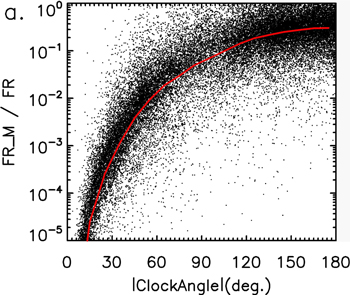
Figure 22. Distributions of the ratio of  as a function of the IMF clock angle
  .
.
Download figure:
Standard image High-resolution imageIt is clear in Figure 22 that, no matter what  is, FR is always larger than
  because the ratio
  is always less than 1. Particularly when
  is greater than 90°, the ratio
  varies from 0.1 to 0.3. Here FR may be overestimated because of the underestimation of the magnetic flux flowing through the flank magnetosheath FSH, since FR = FSW − FSH. The FSH is calculated through FSH = VXBYLSH, where VX and BY are the X component of the plasma velocity and the Y component of the magnetic field in the flank magnetosheath in the SWI coordinate system and LSH is the dimension of the flank magnetosheath along the Z direction. The errors from the dimension LSH are randomly distributed around the real quantities, as shown in Figures 2(d) and (f); thus, the systematic underestimation of FSH might not derive from LSH but from EX = VXBY. In our calculation, EX is assumed to be constant along the Z direction in the flank magnetosheath. This assumption may be too strong, and as in the region close to the magnetopause, EX may be enhanced, that might lead to the underestimation of FSH and overestimation of FR. In this sense, the quantities of FR are only able to be used for a statistical study, and in this paper, their responses to the variations of the outside solar wind conditions are examined, such as in Figure 17.
When  is less than 90°, the ratio
  is very small, and it decreases rapidly as
  decreases (Figure 22). In Figure 17(b), FR is seen to not vary significantly with the variation of
  , and thus the very small
  is due to the small quantity of
  . According to the method to determine
  , it can be understood that
  describes the newly opened magnetic flux added into the polar cap (Milan et al. 2012). However, FR describes a different quantity related to the rate of the magnetopause MR. According to its definition, FR estimates how much of the IMF fluxes go through the magnetosphere per unit time. These fluxes can go through the magnetosphere via the low-latitude MR on the magnetopause when
  is large, and they finally return to the downstream solar wind through MR in the distant tail. These fluxes can also go through the magnetosphere via the lobe MR at high latitudes when
  is small (Song & Russell 1992). In this situation, an IMF field line may reconnect twice at the high latitudes of the opposite pole of the magnetosphere and return back to the solar wind. These high-latitude MRs, typically referred to as "dual MRs," may not add any open flux into the polar cap but produce a newly closed field line wrapping the magnetopause forming the low-latitude boundary layer (Song & Russell 1992). These magnetic fluxes going through the magnetosphere, however, cannot have been involved in
  (Milan et al. 2012), and that is why FR is much larger than
  , particularly when
  is small. In Figure 17(b), it is seen that the rough estimation of FR for the small
  case is equivalent to that for the larger
  case. When
  decreases from 90°, the magnetic shear at high latitudes may increase, leading to the increase in FR as seen in Figure 17(b).
4.5. Controllers of MR Locations on the Magnetopause
Efforts have always been exerted toward looking for the locations where MR is initiated on the magnetopause. It is reasonable to believe that these locations may have some special properties, since MR occurs there but not elsewhere. In the literature, many models have been established to predict the locations of MR or X lines. Usually, MR is treated as the development of a current-driven instability, i.e., the tearing mode instability, the growth rate of which is linked to the current properties across the current sheet (Pudovkin & Semenov 1985; Alexeev et al. 1998). It thus may be reasonable to relate the initiation locations of MR to the electric current  on the magnetopause.
In the present study, a maximum magnetosheath thermal pressure region is found to be located within a belt lying in the subsolar area (Figure 18(a)), and the strongest ion thermal pressure indicates the strongest magnetopause current density  there. Assuming a quasi-steady magnetopause, a balance is achieved through the equal total pressures Pt beside the magnetopause (as seen in Figures 18(c) and (c')), and the flows near the magnetopause are basically tangential to the boundary and thus do not contribute to this balance. The plasma thermal pressure dominates outside the magnetopause, while the magnetic pressure dominates inside the magnetopause (Figures 18(a), (a'), (b), and (b')). The current layer in the subsolar region should be thinnest over the whole magnetopause, and there is no reason to believe that the current layer here could be even thicker, since the total pressure is strongest and the magnetopause is compressed most significantly (Figures 18(c) and (c')). In this circumstance, the strongest thermal pressure gradient across the magnetopause is present in the subsolar region, and it produces the strongest diamagnetic current density. If the local current density
  is great enough to excite the tearing mode instabilities (Pudovkin & Semenov 1985; Alexeev et al. 1998), MR may be initiated. In addition, the sheath flows present in the subsolar sheath region are sub-Alfvénic (as seen in Figures 7 and 19(b)), which is also a favorite condition for the steady MR on the magnetopause (Cowley & Owen 1989; Cooling et al. 2001).
There is another clue for the conjecture that MR is initiated in the strongest magnetopause current region, i.e., in the strongest thermal pressure region. By using the energy dispersion of particles ejected from MR, the location of an X line can be retrieved (Trattner et al. 2007; Zhu et al. 2015). Both the case and statistic studies have revealed that the initial X lines cross the subsolar region, and that their locations shift southward or northward when the dipole tilt axis inclines toward or away from the Sun. The normalized offsets of the retrieved MR sites away from the predicted X lines, which are anchored at the subsolar point, are plotted as a function of the Earth's dipole tilt angle in Figure 6 of Zhu et al. (2015). In this paper, the normalized offsets are converted to be the latitudinal shift angles in the GSM and SWM coordinate systems, and their dependences on the dipole tilt angle are plotted in Figures 23(a) and (b), respectively. It is seen that the latitudinal shift angles of the X lines are comparable to the corresponding dipole tile angles in GSM or SWM (the slopes of the regressing lines in Figure 23 are 1.3 in the GSM coordinate system and 1.2 in the SWM coordinate system). The thermal pressure ridge also shifts southward or northward when the dipole axis rotates toward or away from the Sun, and the slope of the thermal plasma ridge in Figure 20(a) is also about 1, which means that the shift latitudes of the ridge are also equal to the dipole tilt angles. Although the results in this study cannot assert where MR initiates on the magnetopause or distinguish which MR location model is best, the colocalization of the MR initiation sites and the thermal pressure ridge and their dependence on the dipole tilt angle θd suggest that MR tends to occur in association with the thermal pressure ridge, i.e., the strong magnetopause current.

Figure 23. Latitudinal shift angles of X lines away from the modeled X lines, which are anchored at the subsolar point, as a function of dipole tilt angles described in the (a) GSM and (b) SWM coordinate systems. The positive (negative) quantity of the shift angle means that X lines shift southward (northward), and the positive (negative) dipole tilt angle indicates a sunward (tailward) inclination of the dipole axis. The red lines give the linear regressions of the data, and the slopes of the lines are ∼1.3 and ∼1.2 in the GSM and SWM coordinate systems, respectively. The data are the same as used in Figure 6 of Zhu et al. (2015).
Download figure:
Standard image High-resolution imageThe background sheath flow can modify the X-line location, and it can carry an X line away from the subsolar region after the formation of the X line (Raeder 2006). Both Figures 19(a) and 20(e) show that the sheath flows are diverted on the magnetopause, and that the flow stagnation point is persistent at the subsolar point and does not shift away from the subsolar region, no matter what the dipole tilt angle θd is. This phenomenon may derive from the way of the magnetopause reshaping when θd varies. The magnetopause reshapes due to the variation of θd, which can be examined in the MHD simulations done by Liu et al. (2012). Their results show that the magnetopause nose stays persistently around the subsolar point, not depending on θd. The sheath flows are diverted at the nose when they encounter the magnetopause, and that is why the stagnation point remains unchanged as the dipole axis varies (Figure 20(e)). In this scenario, if θd is nonzero, MR will be initiated in the strongest current region away from the subsolar region where the background sheath flow is always present. The background sheath flow may carry the X line further away from the subsolar region, which interpret why the latitudinal shifting angles in Figure 23 are always larger than the corresponding dipole tile angles (the slopes of the regressing lines are greater than 1). One fact should be noted: the probability of θd = 0 is actually very low, and thus they are the most likely locations to investigate the MR triggering processes or initiation conditions.
The background sheath flows present at the MR sites help to produce FTEs. On the basis of MHD simulations, Raeder (2006) proposed that, if θd is nonzero, the background magnetosheath flow carries an X line away from its initiation location, and an FTE forms between the leaving X line and its initiation location when a second X line forms at this location. This scenario is supported by observations provided by Zhang et al. (2012), Zhong et al. (2013), and Pu et al. (2013). The size or duration of an FTE is found to be proportional to the size of the planet's magnetosphere; e.g., the size of the Earth's magnetopause is ∼20 times that of Mercury's magnetopause, and the size/duration of an FTE on the Earth's magnetopause is also 20 times that of an FTE on Mercury (Russell 1995). These observations can be understood in the scenario proposed by Raeder (2006), and the duration of an FTE is actually proportional to the time the first X line takes to move before the second X line forms or the length of the path along which the first X line has moved. Let us assume that the distributions of all kinds of parameters on the Earth's and Mercury's magnetopauses are similar but of different spatial scales. For example, the sheath flow and magnetopause current on the Earth's magnetopause have the same patterns as on Mercury's magnetopause, and the length or time for which the first X line has moved before the second X line forms are then only proportional to the magnetopause's dimensions: the bigger the magnetopause, the longer time/larger distance the first X line may move and the larger the FTE.
5. Summary
In this paper, the properties of the plasma and magnetic field distributions in the magnetosheath are explored, and those properties related to the magnetopause MR are particularly emphasized. The questions that this paper tries to touch on are as follows. (a) To what extent can the solar wind and IMF conditions stand for the inflow condition of MR on the magnetopause? (b) What parameters in the upstream solar wind affect the MR rate on the magnetopause? (c) What parameters affect the locations of MR on the magnetopause? These questions have been studied extensively but remain not fully understood. Although the data and analyses presented in this paper cannot give the ultimate answers to these questions, the magnetosheath properties extracted from these analyses may provide some clues to uncover these mysteries. The findings and main conclusions of this paper are summarized as follows.
- (a)The single upstream solar wind and IMF conditions must be used with caution as the MR initiation conditions on the magnetopause, since the parameters are not evenly distributed in the magnetosheath, and there are asymmetries in the magnetosheath.
- 1.Particularly for the magnetic field–associated parameters, ±Y asymmetries are present in the magnetosheath. These asymmetries are produced by the different types of bow shocks, and the levels of these asymmetries are controlled by the IMF cone angle θCO.
- 2.The weak ±Y asymmetries exist in the distributions of the plasma parameters, and these asymmetries are mainly produced within the magnetosheath.
- 3.The Y–Z asymmetries are present in the magnetosheath, and these asymmetries are produced by further diversion, compression, and reacceleration.
- 4.The key parameters to the MR initiation or proceeding, such as the field line bending (φm,X and φm,YZ), which is determinative of the magnetic shear angle θX at the magnetopause, and the plasma β, are asymmetrically distributed outside the magnetopause.
- (b)The IMF magnetic flux passing through the magnetosphere, FR, is estimated in this study, and its dependence on outside conditions is examined. Notice that, according its definition, FR not only includes the newly opened magnetic flux added into the polar cusp but also involves the magnetic flux reconnected at high latitudes via the dual-lobe MR (Song & Russell 1992).
- 1.The IMF clock angle θCL, magnetosheath plasma β, and solar wind sound Mach number MS are the three critical parameters to control FR.
- 2.The magnetic fluxes going through the magnetosphere, FR, are comparable for the cases with
 > 90° and <90°, and FR increases when increases from 90° to 180° or decreases from 90° to 0°.
 - 3.The magnetosheath plasma β is the other key parameter to control FR. The upstream solar wind parameters control the magnetosheath plasma β, and a small IMF cone angle, strong IMF strength , small solar wind plasma βSW, or strong solar wind convection electric field produce a small plasma β just outside the magnetopause, leading to a large FR.
- 4.The solar wind sound Mach number MS is independent of the subsolar magnetosheath plasma β, but MS controls the global parameter FR through modifying the magnetosheath plasma β at high latitudes or the flank magnetopause. A high effective MS may produce a highly compressed plasma at high latitudes or the flank magnetopause, leading to a large β there, which reduces the global FR.
- 5.Under a more radial IMF (a larger) condition, the magnetopause may expand in all directions. The larger corresponds to the less compressed sheath magnetic field, higher magnetosheath β, lower magnetopause MR rate FR, lower magnetosheath total pressure, larger and more flaring magnetopause, and wider strongly compressed sheath plasma region. All of these observational phenomena are self-consistent.
- (c)The dipole tilt angle, the property from the inside magnetosphere, is a factor affecting the magnetosheath parameter distributions in the SWM coordinate system.
- 1.The colocalization of the thermal pressure ridge and MR initiation sites and their dependence on the dipole tilt angle θd suggest that MR tends to occur in association with the thermal pressure ridge, i.e., the strong magnetopause current.
- 2.The stagnation line of the sheath flow is observed to be anchored persistently at the subsolar point, and the dipole tilt angle θd cannot adjust its location. The background sheath flows are thus present at the location of an X line if. This background flow may carry the X line from its initial location to higher latitudes, and a second X line may form at this location; in this scenario, an FTE can be generated by MR at the two sequentially formed X lines.


This work is supported by the National Science Foundation of China (41731068, 41774175, and 41621063). The authors thank the FGM and CIS instrument teams of Cluster and the FGM and ESA instrument teams of THEMIS for providing data and the NASA/GSFC's Space Physics Data Facility for the OMNIWeb service. The OMNI data are available at http://cdaweb.gsfc.nasa.gov/cgi-bin/eval1.cgi. The authors are especially grateful to Dr. Khurana K. Krishan of UCLA for his insightful and useful suggestions for this paper.